Switching Extended Kalman Filter Bank for Indoor Localization Using Wireless Sensor Networks

Abstract

This paper presents a new filtering algorithm, switching extended Kalman filter bank (SEKFB), for indoor localization using wireless sensor networks. SEKFB overcomes the problem of uncertain process-noise covariance that arises when using the constant-velocity motion model for indoor localization. In the SEKFB algorithm, several extended Kalman filters (EKFs) run in parallel using a set of covariance hypotheses, and the most probable output obtained from the EKFs is selected using Mahalanobis distance evaluation. Simulations demonstrated that the SEKFB can provide accurate and reliable localization without the careful selection of process-noise covariance.

1. Introduction

Localization involves tracking locations of objects that are of interest, such as robots, humans, vehicles, and equipment [1,2,3]. Outdoor localization usually depends on a global positioning system, whereas indoor localization exploits various types of wireless sensor networks (WSNs) [4]. A typical WSN comprises several fixed nodes installed at designated locations and mobile nodes attached to target objects. Fixed and mobile nodes communicate with each other using wireless signals, and the locations of mobile nodes are obtained by analyzing the parameters of wireless signals. Time of arrival (TOA) [5], time difference of arrival (TDOA) [6], and angle of arrival [7] are typical wireless measurements used for indoor localization.

A wireless measurement is corrupted by noise, which is inevitable but can be mitigated using stochastic filters (also referred to as state estimators). To exploit stochastic filters, a localization system should be modeled in a state space form that comprises motion and measurement models. Because wireless measurements of WSNs are typically represented by nonlinear measurement models, nonlinear stochastic filters such as the extended Kalman filter (EKF) and the particle filter (PF) are often used for indoor localization [8,9,10,11]. In this study, the EKF was used for indoor localization because it has an advantage over the PF in terms of real-time processing.

In indoor localization, the constant-velocity (CV) motion model is commonly used to represent the motion of target objects. In the CV motion model, process-noise covariance $\mathbf{Q}$ plays a critical role, but it is a highly uncertain design parameter [12,13,14,15]. The conventional EKF algorithm uses constant $\mathbf{Q}$ values that are selected on the basis of an engineer’s knowledge and experience. However, inappropriately selected $\mathbf{Q}$ may degrade localization accuracy [12,13].

Uncertainty in the motion model is one of the oldest problems in the field of target tracking. To solve this problem, interacting multiple model (IMM) filtering [16] was developed. IMM filtering mixes models for which mixing probabilities are computed using the probabilities of transition between multiple models. Transitional probability (TP) is a key design parameter in IMM filtering. Guidelines to designing TP were presented for typical motion models used in target tracking, for example, CV motion and coordinated turn motion models [14,15]. However, TP design is still a cumbersome problem. In particular, it is difficult to design a TP between different $\mathbf{Q}$ values in the same CV motion model. Thus, a filtering algorithm that is simple and easy to implement is required for indoor localization.

This paper proposes a new filtering algorithm, the switching extended Kalman filter bank (SEKFB), to overcome the uncertain process-noise covariance problem. In the SEKFB algorithm, a filter bank consisting of several EKFs is constructed. EKFs in the filter bank use different $\mathbf{Q}$ hypotheses that are roughly selected without careful consideration or experience. In addition, the most probable among EKF outputs is selected using Mahalanobis distance evaluation [17]. SEKFB thereby alleviates the problem of selecting $\mathbf{Q}$ and designing the TP. Without the need for the careful selection of $\mathbf{Q}$, the SEKFB algorithm performs accurate localization compared to the best achieved performance of an EKF. In addition, the SEKFB provides reliable localization, while the conventional EKF exhibits localization failures. Moreover, the SEKFB is easy to implement because of its simple algorithm. The excellent performance of the SEKFB is demonstrated via the simulation of indoor localization using a WSN.

The remainder of this paper is organized as follows. Section 2 discusses the indoor localization scheme utilizing the EKF, and proposes the SEKFB. Section 3 presents simulation results for the demonstration of SEKFB performance. Lastly, the conclusions of the study are presented in Section 4. The abbreviations used in this paper are listed in

Table 1. List of abbreviations.

Abbreviations	Explanation
CV	Constant velocity
EKF	Extended Kalman filter
IMM	Interactive multiple model
MC	Monte Carlo
RMSPE	Root-mean-square position error
RTAMSE	Root-time-averaged mean square error
SEKFB	Switching extended Kalman filter bank
TDOA	Time difference of arrival
TOA	Time of arrival
TP	Transition probability
WSN	Wireless sensor network

.

2. Indoor Localization Scheme and Proposed Algorithm

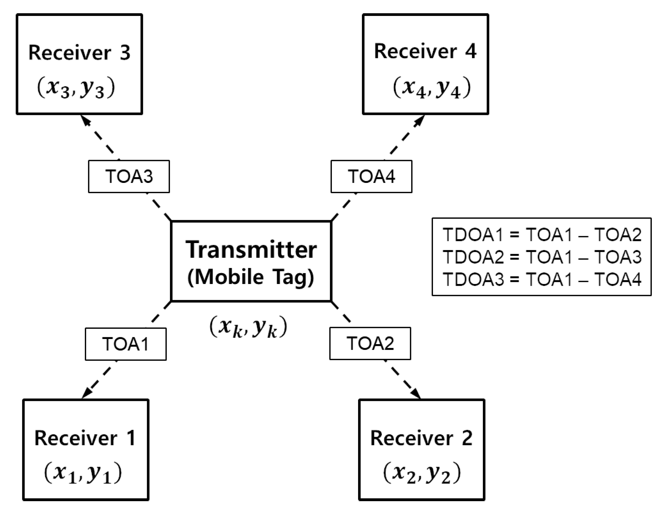
We considered an indoor localization system using a WSN described as follows. To simplify the problem, the indoor space was assumed to be a two-dimensional (2D) floor space. Figure 1 shows the configuration of a WSN using TDOA measurements.

Four receivers were installed at designated locations in the indoor space. A transmitter (mobile tag) was attached to a target object (e.g., vehicles, equipment, or human) in the space. The four receivers received signals from the transmitter and measured four TOAs that are defined as follows:

$$\begin{array}{cc}\hfill {\mathrm{TOA}}_{i,k}& =\frac{1}{c}{d}_{i,k},i=1,2,3,4,\hfill \end{array}$$

(1)

$$\begin{array}{cc}\hfill d_{i,k}& =\sqrt{{(x_k-x_i)}^2+{(y_k-y_i)}^2},\hfill \end{array}$$

(2)

where c is the speed of light; $d_i$ is the distance between transmitter and i-th receiver; $(x_k,y_k)$ are the 2D positions of the transmitter at time k; and $(x_i,y_i)$ are the fixed positions of the receivers. The receiver’s clocks were synchronized with each other. The measured TOAs were transmitted to a server computer, and the TDOA was computed as follows:

$$\begin{array}{cc}\hfill {\mathrm{TDOA}}_{i,k}& ={\mathrm{TOA}}_{1,k}-{\mathrm{TOA}}_{i+1,k},i=1,2,3.\hfill \end{array}$$

(3)

Because TDOA measurements are corrupted by noise, the EKF was used to estimate the target positions from noisy measurements. At each time step k, the EKF performs two processes, time and measurement updates. In the time-update process, state variables are updated using a motion model. We used the CV motion model for updating, and state variables to be estimated were 2D positions $(x,y)$ and velocities $(v_x,v_y)$ as shown in Figure 2.

State variables at time k are represented as $(x_k,y_k)$ and $(v_{x,k},v_{y,k})$. To simplify the notation of velocities, we used $({\dot{x}}_k,{\dot{y}}_k)$ instead of $(v_{x,k},v_{y,k})$. Thus, state vector ${\mathbf{x}}_k$ was constructed as ${\mathbf{x}}_k\triangleq {\left[x_k{y}_k{\dot{x}}_k{\dot{y}}_k\right]}^T$. Thus, the CV motion model [14,15] is represented as

$$\begin{array}{cc}\hfill {\mathbf{x}}_{k+1}& =\mathbf{A}{\mathbf{x}}_k+\mathbf{G}{\mathbf{w}}_k,\hfill \\ \hfill \mathbf{A}& =\left[\begin{array}{cccc}1& 0& T& 0\\ 0& 1& 0& T\\ 0& 0& 1& 0\\ 0& 0& 0& 1\end{array}\right],\mathbf{G}=\left[\begin{array}{cc}{T}^2/2& 0\\ 0& T^2/2\\ T& 0\\ 0& T\end{array}\right],\hfill \end{array}$$

(4)

where T is the sampling interval, and ${\mathbf{w}}_k$ is the process-noise vector. We assumed that ${\mathbf{w}}_k$ was zero-mean white Gaussian noise with covariance matrix $\mathbf{Q}=q{\mathbf{I}}_2$, where ${\mathbf{I}}_2$ is a $2\times 2$ identity matrix.

The measurement update process of the EKF uses a measurement model. The TDOA measurements are expressed as

$$\begin{array}{c}\hfill \left[\begin{array}{c}{z}_{1,k}\\ z_{2,k}\\ z_{3,k}\end{array}\right]=\left[\begin{array}{c}{h}_{1,k}\\ h_{2,k}\\ h_{3,k}\end{array}\right]=\frac{1}{c}\left[\begin{array}{c}{d}_1-d_2\\ d_1-d_3\\ d_1-d_4\end{array}\right],\end{array}$$

(5)

where $z_{1,k},z_{2,k}$, and $z_{3,k}$ are TDOA measurements (in units of nanoseconds); $h_{1,k},h_{2,k}$, and $h_{3,k}$ are nonlinear measurement equations that produce TDOA measurements. The measurement vector and measurement equation vector were constructed as ${\mathbf{z}}_k={\left[z_{1,k}{z}_{2,k}{z}_{3,k}\right]}^T$ and ${\mathbf{h}}_k={\left[h_{1,k}{h}_{2,k}{h}_{3,k}\right]}^T$, respectively. The measurement model can then be expressed as

$$\begin{array}{cc}\hfill {\mathbf{z}}_k& ={\mathbf{h}}_k\left({\mathbf{x}}_k\right)+{\mathbf{v}}_k,\hfill \end{array}$$

(6)

where ${\mathbf{v}}_k$ is the Gaussian measurement noise vector with covariance $\mathbf{R}$.

Given the motion and measurement models, the EKF was used to estimate the 2D positions of the transmitter. EKF equations for the state-space models (4) and (6) are represented as follows:

$$\begin{array}{cc}\hfill {\widehat{\mathbf{x}}}_k^{-}& =\mathbf{A}{\widehat{\mathbf{x}}}_{k-1}^{+},\hfill \end{array}$$

(7)

$$\begin{array}{cc}\hfill {\mathbf{P}}_k^{-}& =\mathbf{A}{\mathbf{P}}_{k-1}^{+}{\mathbf{A}}^T+\mathbf{G}\mathbf{Q}{\mathbf{G}}^T,\hfill \end{array}$$

(8)

$$\begin{array}{cc}\hfill {\mathbf{K}}_k& ={\mathbf{P}}_k^{-}{\mathbf{H}}^T{(\mathbf{H}{\mathbf{P}}_k^{-}{\mathbf{H}}^T+\mathbf{R})}^{-1},\hfill \end{array}$$

(9)

$$\begin{array}{cc}\hfill {\widehat{\mathbf{x}}}_k^{+}& ={\widehat{\mathbf{x}}}_k^{-}+{\mathbf{K}}_k({\mathbf{z}}_k-\mathbf{H}{\widehat{\mathbf{x}}}_k^{-}),\hfill \end{array}$$

(10)

$$\begin{array}{cc}\hfill {\mathbf{P}}_k^{+}& =(\mathbf{I}-{\mathbf{K}}_k\mathbf{H}){\mathbf{P}}_k^{-},\hfill \end{array}$$

(11)

where ${\mathbf{P}}_k$ is the estimation error covariance matrix; ${\mathbf{K}}_k$ is the Kalman gain; and superscripts − and + represent a priori and a posteriori, respectively. $\mathbf{H}$ is the Jacobian matrix defined as

$$\begin{array}{cc}\hfill {\mathbf{H}}_k& ={\left.\frac{\partial {\mathbf{h}}_k}{\partial \mathbf{x}}\right|}_{{\widehat{\mathbf{x}}}_k},\hfill \end{array}$$

(12)

and obtained as follows:

$$\begin{array}{cc}\hfill {\mathbf{H}}_k& =\left[\begin{array}{cccc}{h}_{11,k}& h_{12,k}& 0& 0\\ h_{21,k}& h_{22,k}& 0& 0\\ h_{31,k}& h_{32,k}& 0& 0\end{array}\right],\hfill \\ \hfill h_{11,k}& =\frac{1}{c}\left(\frac{x_k-x_1}{d_1}-\frac{x_k-x_2}{d_2}\right),\hfill \\ \hfill h_{12,k}& =\frac{1}{c}\left(\frac{y_k-y_1}{d_1}-\frac{y_k-y_2}{d_2}\right),\hfill \\ \hfill h_{21,k}& =\frac{1}{c}\left(\frac{x_k-x_1}{d_1}-\frac{x_k-x_3}{d_3}\right),\hfill \\ \hfill h_{22,k}& =\frac{1}{c}\left(\frac{y_k-y_1}{d_1}-\frac{y_k-y_3}{d_3}\right),\hfill \\ \hfill h_{31,k}& =\frac{1}{c}\left(\frac{x_k-x_1}{d_1}-\frac{x_k-x_4}{d_4}\right),\hfill \\ \hfill h_{32,k}& =\frac{1}{c}\left(\frac{y_k-y_1}{d_1}-\frac{y_k-y_4}{d_4}\right).\hfill \end{array}$$

(13)

Process-noise covariance $\mathbf{Q}$ in (8) had a significant effect on EKF performance. $\mathbf{Q}$ was derived from the CV motion model and is related to the movement rate of a target. Because the movement of a target (e.g., person) is unpredictable, selecting a suitable $\mathbf{Q}$ is difficult. If an unsuitable $\mathbf{Q}$ value is used, EKF accuracy degrades. Thus, we propose the SEKFB algorithm, which can provide accurate and reliable localization without selecting a suitable $\mathbf{Q}$. 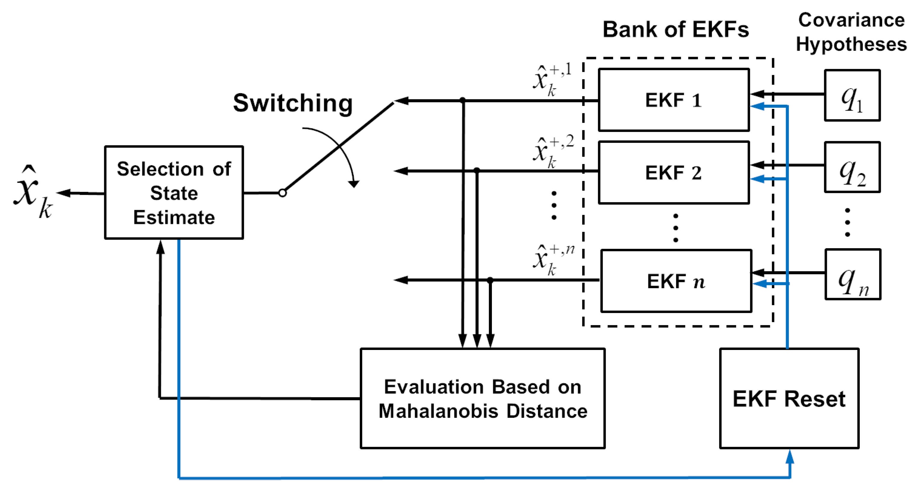Figure 3 illustrates the structure of SEKFB. EKFs using different process noise covariances constitute a filter bank. State estimates of EKFs are evaluated using Mahalanobis distance. The best estimate is selected as the output of SEKFB, and it is also used to reset the EKFs.

The first step of the SEKFB algorithm is to select $\mathbf{Q}$ hypotheses, which involves selecting q hypotheses because we assumed that $\mathbf{Q}=q{\mathbf{I}}_2$. We constructed set of hypotheses $\{q_1,q_2,\cdots ,q_n\}$, where n is the number of hypotheses. Hypotheses do not need to be selected in a careful manner. Designers can roughly select the hypotheses (e.g., $q=1,10,100,\cdots$), and the hypotheses perform suitably owing to the SEKFB algorithm.

In the next step, n EKFs using the n hypotheses are operated in parallel. At each time step, n state estimates $\{{\widehat{\mathbf{x}}}_k^{+,1},{\widehat{\mathbf{x}}}_k^{+,2},\cdots ,{\widehat{\mathbf{x}}}_k^{+,n}\}$ are obtained. The best state estimate is selected by minimizing Mahalanobis distance between actual TDOA measurement ${\widehat{\mathbf{z}}}_k$ and predicted measurements ${\widehat{\mathbf{z}}}_k^j$, where $j=1,2,\cdots ,n$. The predicted measurement is computed using the state estimate as follows:

$$\begin{array}{cc}\hfill {\widehat{\mathbf{z}}}_k^j& ={\mathbf{h}}_k\left({\widehat{\mathbf{x}}}_k^{+,j}\right),\end{array}$$

(14)

where ${\widehat{\mathbf{x}}}_k^{+,j}$ is the state estimate obtained from the j-th EKF. Mahalanobis distance [17] is computed as

$$\begin{array}{c}\hfill {\mathcal{D}}_k^j={({\mathbf{z}}_k-{\widehat{\mathbf{z}}}_k^j)}^T{\mathbf{R}}^{-1}({\mathbf{z}}_k-{\widehat{\mathbf{z}}}_k^j).\end{array}$$

(15)

If the j-th EKF produces the minimal ${\mathcal{D}}_k^j$, ${\widehat{\mathbf{x}}}_k^{+,j}$ is chosen as the output of the SEKFB at time k. For the estimation of the next time step $k+1$, the other EKFs except the j-th EKF are reset using the information of the most reliable EKF. Thus, EKFs can produce more reliable estimates than those estimated using previous algorithms. The overall algorithm of the SEKFB is summarized in Algorithm 1.

Algorithm 1: Filtering using SEKFB.

3. Simulation

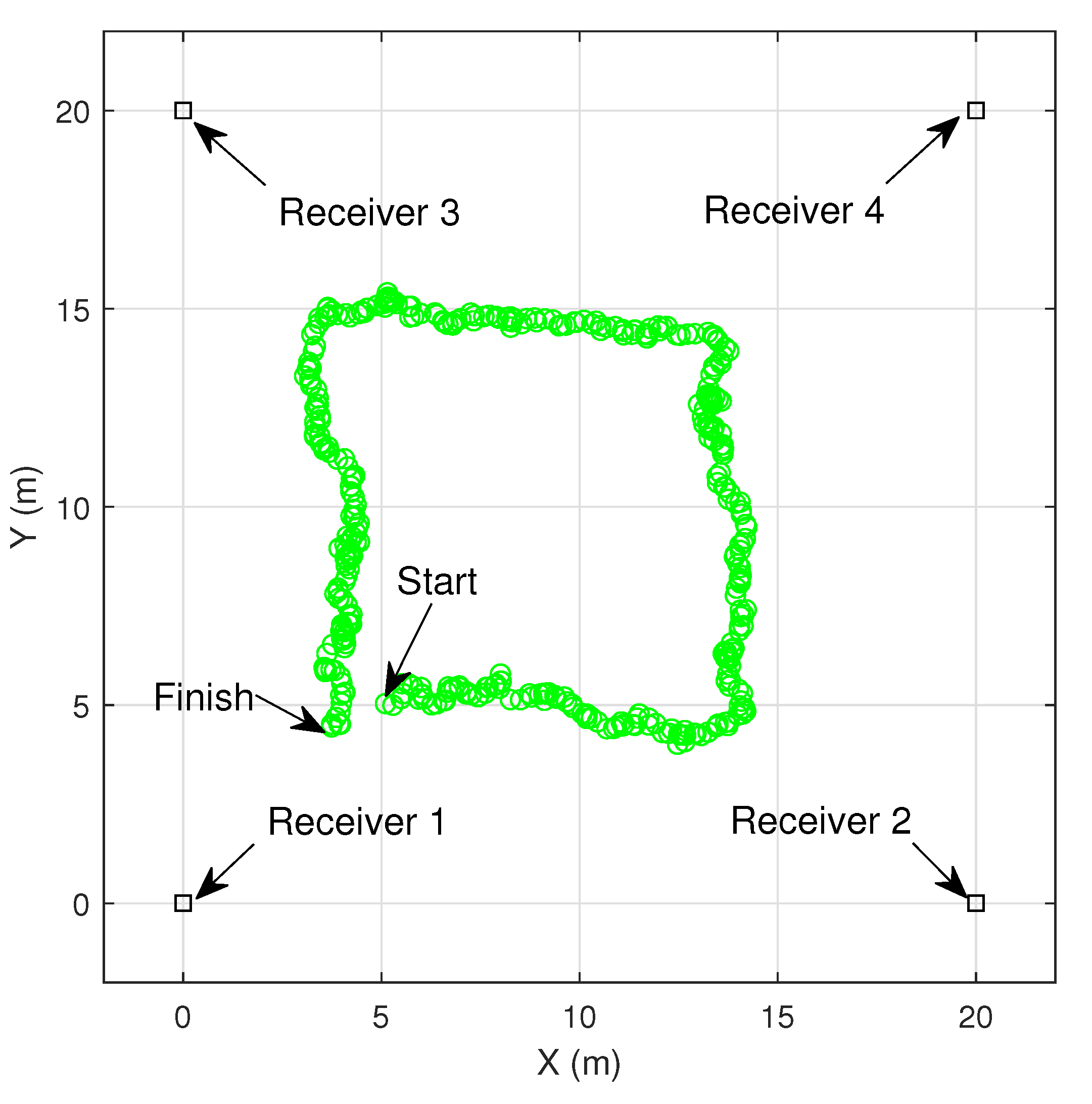
We simulated indoor localization using SEKFB. The simulation scenario was as follows. A person equipped with a mobile tag (transmitter) traveled along a square trajectory in an indoor space as shown in Figure 4. The size of the indoor space was $20\times 20$ m. Four receivers were installed at positions $(0,0)$, $(0,20)$, $(20,0)$, and $(20,20)$ m. The receivers obtained wireless signals from the transmitter, and three TDOA measurements were acquired as shown in Figure 1.

At each time step, the 2D positions of a person $(x_k,y_k)$ were estimated using both the SEKFB and conventional EKFs. Motion and measurement models given in (4) and (6), respectively, were used for the filters. In the simulation, TDOA measurements were generated using the measurement model given in (6), and measurement-noise covariance $\mathbf{R}=0.1^2{\mathbf{I}}_3$. We assumed that measurement-noise covariance was exactly known. However, process-noise covariance $\mathbf{Q}$ was unknown. Thus, we roughly selected q hypotheses as $\{100,10,1,0.1,0.01\}$. We operated the EKF using the five q hypotheses to find the best performing hypothesis. Next, we operated the SEKFB and compared its performance with the best achievable performance of the EKF.

Filter performance was evaluated by the root-mean-square position error (RMSPE) and root time-averaged mean square error (RTAMSE). We ran 100 Monte Carlo (MC) simulations. RMSPE at time k and RTAMSE were calculated as

$$\begin{array}{cc}\hfill {\mathbf{RMSPE}}_k& =\frac{1}{N_e}\sum _{m=1}^{N_e}\sqrt{{(x_k^m-{\widehat{x}}_k^m)}^2+{(y_k^m-{\widehat{y}}_k^m)}^2},\hfill \end{array}$$

(16)

$$\begin{array}{cc}\hfill \mathbf{RTAMSE}& =\frac{1}{N_e{t}_{\max }}\sum _{m=1}^{N_e}\sum _{k=1}^{t_{\mathrm{final}}}\sqrt{{(x_k^m-{\widehat{x}}_k^m)}^2+{(y_k^m-{\widehat{y}}_k^m)}^2},\hfill \end{array}$$

(17)

where $t_{\mathrm{final}}$ is the final time step, $N_e$ is the number of effective simulations, and $N_e=100-N_f$, where $N_f$ is the number of localization failures. A case that produced the RTAMSE at a value greater than $5m$ was considered to be a localization failure.

Figure 5a shows the RMSPEs of the EKFs using the five q hypotheses. $q=0.01$ produced the largest RMSPE, that is, the worst performance. $q=10$ and $q=100$ produced much smaller RMSPEs compared with the other q hypotheses. Because RMSPEs produced by $q=10$ and $q=100$ were similar and difficult to distinguish, we compared their RTAMSEs.

Table 2. Root time-averaged mean square error and number of localization failures.

Filter	RTAMSE	Number of Localization Failures
SEKFB	0.0249	0
EKF ($q=100$)	0.0260	6
EKF ($q=10$)	0.0252	1
EKF ($q=1$)	0.0626	0
EKF ($q=0.1$)	0.2199	0
EKF ($q=0.01$)	0.7045	0

compares the RTAMSEs of the filters; $q=10$ and $q=100$ produced RTAMSE values of $0.0252$ and $0.0260$, respectively. Thus, the best EKF performance could be achieved with $q=10$.

In Figure 5b, we compared the SEKFB and EKF with $q=10$. The two filters exhibited similar RMSPEs, as shown in Figure 5b, and we compared them in terms of the RTAMSE. As shown in Table 2, the RTAMSE of the SEKFB was $0.0249$, which was smaller than that of the EKF with $q=10$. The best choice for q was unknown in advance. The process-noise covariance of the CV model is a highly uncertain design parameter, and selecting an appropriate covariance value is difficult. EKF performance with $q=10$ or $q=100$ could be obtained when a selected covariance value is appropriate. However, the SEKFB exhibited accurate localization performance without selecting an appropriate covariance value.

We compared the filters in terms of the number of localization failures as shown in Table 2. EKFs using $q=10$ and 100 produced RTAMSEs similar to those of the SEKFB, but they exhibited localization failures. However, the SEKFB did not fail, which means that the SEKFB was more reliable than EKFs using constant q values are. Thus, simulation results demonstrated that SEKFB is more accurate and reliable than a conventional EKF that uses constant covariance is.

Lastly, we compared the SEKFB with the IMM EKF under various signal-to-noise ratio (SNR) conditions. The IMM EKF algorithm ran five EKFs in parallel. Each EKF matched to the CV motion models using different process-noise covariances. The same q values were used for the IMM EKF as those used for the SEKFB. The IMM algorithm required elaborate TP design, but information on TP between the five motion models was completely unknown. Hence, we assumed that the five CV motion models had the same probabilities. 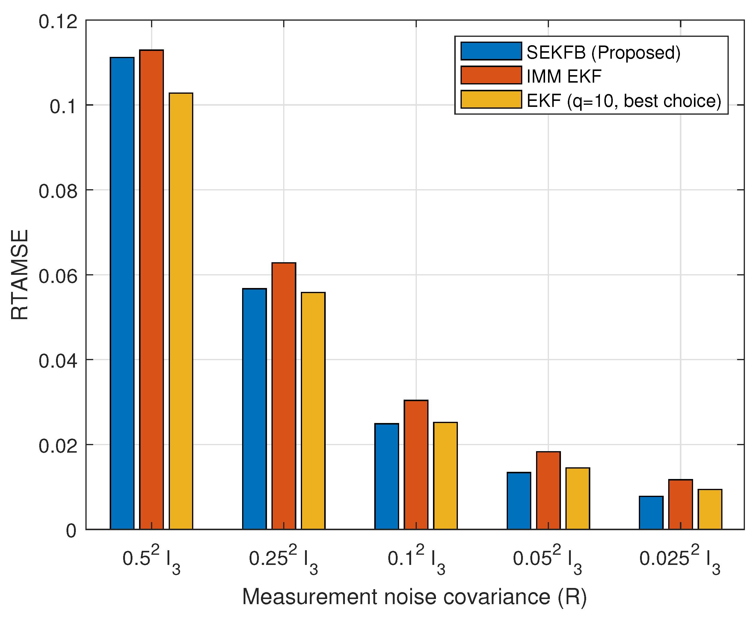Figure 6 compares the RTAMSEs of the SEKFB, IMM EKF, and EKF using the best q value. For various SNR conditions, we used five different measurement-noise covariances as $\mathbf{R}=r^2{\mathbf{I}}_3$, where $r=0.5$, $0.25$, $0.1$, $0.05$, and $0.025$. SNR increased as r decreased. In Figure 6, RTAMSEs tended to decrease as r decreased, which indicates that localization accuracy increased as SNR increased. The SEKFB exhibited smaller RTAMSEs than the IMM EKF did because the SEKFB selects the most suitable q at each time step on the basis of Mahalanobis distance, but the IMM EKF cannot. Under high SNR conditions, for example, $r=0.05$ and $0.025$, the SEKFB was more accurate than the EKF using best constant q was because the adaptation of q in the SEKFB algorithm was based on Mahalanobis distance evaluation. When computing the Mahalanobis distance, predicted measurement ${\widehat{\mathbf{z}}}_k$ was obtained while ignoring measurement noise. Errors due to ignorance may be small under low-measurement-noise (i.e., high SNR) conditions. Thus, the SEKFB is more effective under high SNR conditions.

4. Conclusions

This paper proposed SEKFB for indoor localization using a WSN. The SEKFB switches multiple $\mathbf{Q}$ hypotheses in the CV motion model, whereas conventional algorithms use constant $\mathbf{Q}$ values. In the simulation, the SEKFB exhibited excellent localization accuracy without a priori information on the best covariance value. SEKFB accuracy was better than that of the IMM EKF. Moreover, the SEKFB exhibited better reliability than that of the conventional EKF in terms of localization failure. The SEKFB can thus provide more accurate and reliable performance than conventional EKFs can for indoor localization using WSNs.