1. Introduction
With the breakthrough of Artificial Intelligence (AI), technology is swiftly progressing—from traditional machine learning methods to deep learning methods that uses neural networks (NNs) and from image classification networks to object detection networks. Additionally, the technological evolutions of both hardware and software designs have enabled AI networks to own the capability to judge just like human beings, or sometimes, even better than human beings.
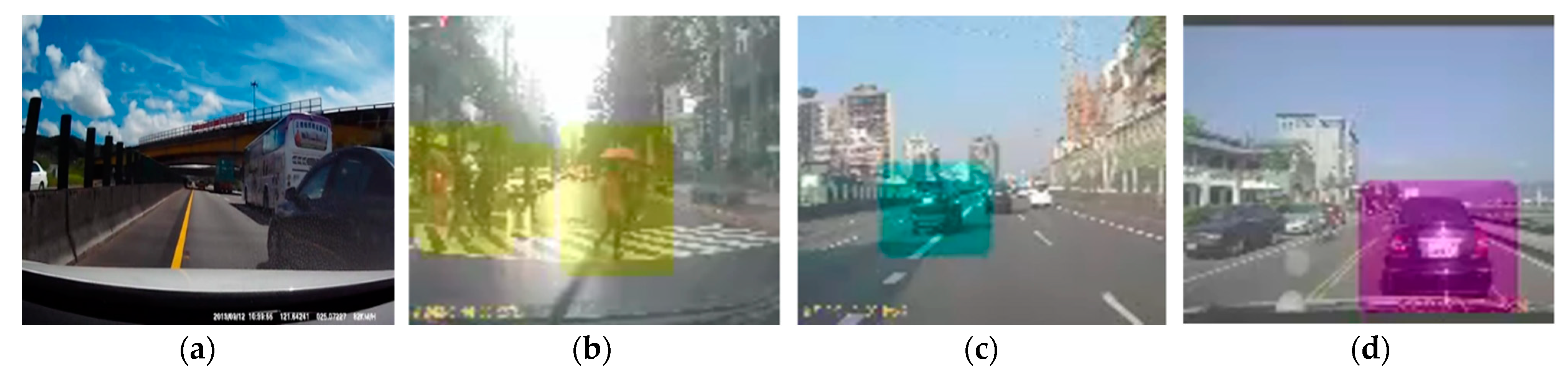
Advanced Driving Assistance Systems (ADAS) are electronic systems embedded as a crucial part of modern day motor vehicles, increasing not just the user-friendliness of the motor vehicles but also enhancing the overall safety of the passengers as well as the pedestrians. The ADAS systems are expected to decrease the damage to roads and other probable properties in driving environments, occurring due to crashes and other accidents, by maximizing the human-vehicle interaction, and sometimes autonomously changing motor vehicles behavior to prevent risks and crashes. Various ADAS applications adapting NNs have been flourishing rapidly in recent years. In order to let the individuals driving motor vehicles become capable of avoiding potential risks and dangers, it is desirable to have a highly accurate ADAS system to assess any situation in real-time while driving and alert the driver, and at times take certain decisions. A group of applications such as the detection of lanes, obstacles, traffic signs, and many more in real-time driving environments can be detected just by perceiving their positions, although there exist certain limitations where not all these applications are favored by drivers [
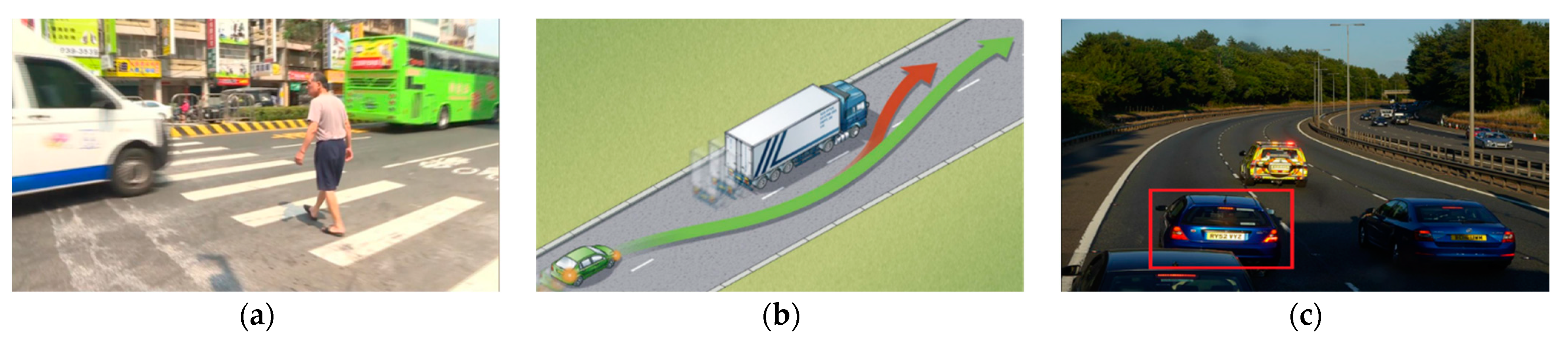
1]. However, certain scenarios on roads, such as pedestrian crossings (as shown in
Figure 1a), cars cutting-in quickly to the lanes ahead [
2] (as in
Figure 1b), and cars ahead applying emergency brakes [
3] (as in
Figure 1c), require a stable, accurate predictive method to evaluate the behavior of the aforementioned moving objects so as to determine the behavior and direction of the motion of pedestrians, scooters, motorcycles, and vehicles to avoid feasible uncertainties and accidental dangers.
Breakthroughs in the application of image classifications and object detections are rapidly maturing. Since the introduction of AlexNet [
4] in 2012, NNs for image classification based on AlexNet, like ZF-net [
5] or VGG [
6], distinctly evolved in terms of object detection and classification. The newest of the NNs of object detection, like Single-Shot MultiBox detectors (SSD) [
7] and You Only Look Once (YOLO) [
8], achieve amazing accuracy with faster computational speed. However, most of the above-mentioned networks just focus on a single image classification and object detection. With further evolutions in the fields of image classification and object detection, researchers are challenging more complicated issues related to behavioral detection. The temporal feature information [
9,
10,
11,
12,
13,
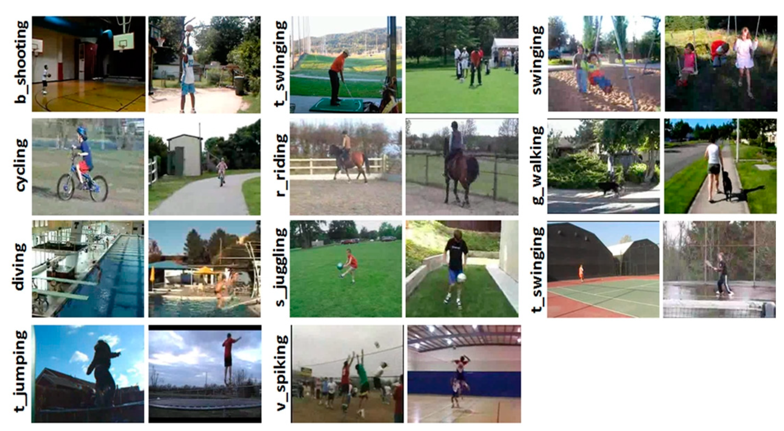
14] in the behavior NNs predicts the behavior that may happen with a preparatory action. Behavior recognition should not only recognize if the specific object exists in images but also predict if the specific object is performing a particular behavior in the image, as extracted from the UCF101-action recognition dataset (University of Central Florida 101) [
15] shown in
Figure 2. Behavior detection should detect not only the position of specific objects in images, but also the specific behavior of the objects in the images.
However, the existing behavior recognition or detection NNs focus largely on specific mankind or sports activities. Moreover, a large number of current action recognition NNs [
16,
17,
18,
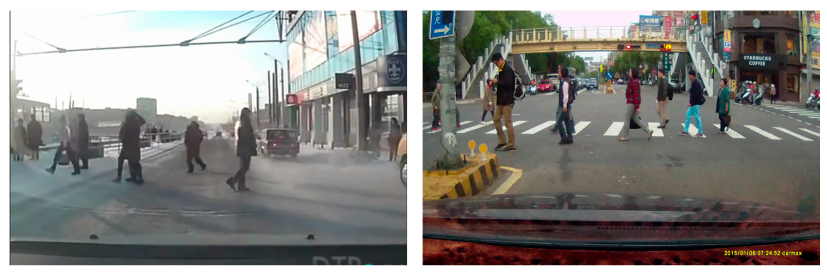
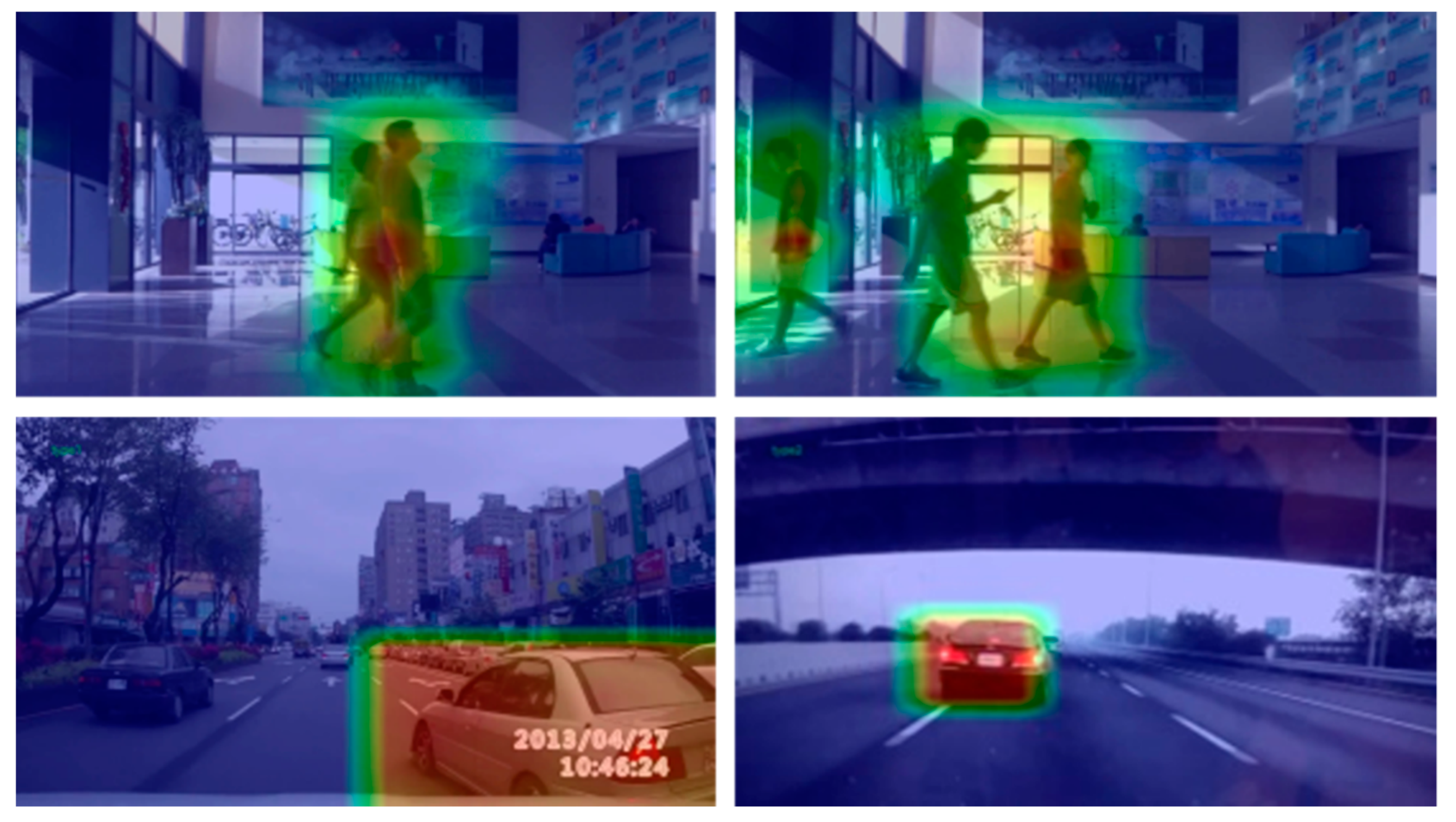
19] are concentrated on offline video recognition rather than real-time behavior recognition. In order to implement the behavior NNs on ADAS, it is a requisite to have a real time, high accurate, and reliable model. Moreover, there are diversified situations that occur while driving, such as many people crossing roads at the same time, as shown in
Figure 3. If a single model is used to learn every solitary behavior of individuals or vehicles in real-traffic environments, it consumes an abundance of time and requires higher processing capabilities. Therefore, this paper proposes an NN model capable of detecting multiple behaviors of distinct objects simultaneously in real time, as prescribed for real-time ADAS applications.
2. Background
The NNs employed for behavior recognitions can be broadly classified into two major types: behavior recognition based on 2D convolution and behavior recognition based on 3D convolution. The behavior recognition based on 2D convolution has a lesser number of parameters than the latter. Further, behavior recognition based on 2D convolution can conveniently use a pre-trained model from 2D image recognition. However, certain additional efforts are necessary to obtain and maintain the temporal information [
8]. On the other hand, behavior recognition based on 3D convolution can easily get temporal information by just performing convolution but the 3D convolution always suffers from a large number of parameters and requires supplemental efforts to fit a 2D pre-trained model into a 3D network structure.
For any kind of behavior recognition, temporal information is necessary. However, the process of behavior recognition based on 2D convolution solely extracts spatial features and hence it needs other ways to obtain temporal information.
The two stream convolution network [
20] divides the task into two NNs, of which the first is a spatial stream network that performs traditional image recognition and is responsible for extracting spatial features. It analyzes information from every frame and situation. Whereas, the second is a temporal stream network, which is a 2D convolution network using stacking optical flow as input. The temporal stream network observes the movement information of camera and objects and then a support vector module (SVM) fuses the information from these two NNs.
Long-term recurrent convolutional networks (LRCN) [
21] support changeable inputs and outputs. This network is an end-to-end trainable network. The recurring neural network (RNN) unit has problems with temporal gradient that cause the adoption of LSTM unit instead of an RNN unit.
Of the three gates in long short-term memory (LSTM) [
22], the memory units and gates enable LSTM to learn ‘when to forget previous information’ and ‘when to refresh status’. Thus, the time information passed is longer. Since LSTM has changeable inputs and outputs, it yields good accuracy on both behavior recognition and video captioning. However, when applied to behavior recognition, the numbers of CNNs are equivalent to the number of sequential frames. Although it has good recognition accuracy, its computational time cost increases with the number of frames.
Temporal Segment Networks (TSN) [
23] have impressive improvements in terms of efficiency and processing. The key idea of this network is in its method of sparsely sampling clips across the video, instead of randomly sampling across the entire video. Each input video is divided into segments and one of the frames from these segments is randomly selected so that the model can get better temporal information. The TSN uses two convolution networks, i.e., spatial and temporal networks to extract temporal information. The selected frame acts as the input for spatial convolution networks and the optical flow of the selected frame is the input for temporal convolution networks. After convolution networks, it agrees with all the segments of temporal and spatial convolution independently by averaging across all the segments. Finally, when class scores fusion occurs, it makes the final decision on behavior by using weighted average and applying softmax over all classes.
The Temporal Shift Module (TSM) [
12] uses a unique new module, which can mix the features of different frames. This enables the 2D convolution to learn information from different times and extract features with temporal information like 3D convolution does. After convoluting each frame in 2D, the features with multiple channels for each frame are obtained. The convolution is divided into two parts: (i) the shift part and (ii) the multiply-accumulate part. Most of the computational cost is spent on the multiply-accumulate part, while the cost of the shift part is extremely small. The TSM can be viewed as a temporal information extract module, which has nearly zero cost. The existence of TSM does not result in shape change of features, so it can be inserted into any 2D convolution network, like ResNet [
12]. The TSM ResNet [
12] has far less parameters than 3D convolution networks and has accuracy better than some 3D convolution networks.
The 3D convolution method is an easy and straightforward, yet powerful approach to draw temporal and spatial features simultaneously. The 3D convolution utilizes deep convolution that particularly possesses filters in three dimensions and yields a faster speed, compared to 2D convolution behavior recognition methods in the early stages. Nonetheless, it incurs a higher computational cost and demands a huge number of parameters in the model, which in turn involves challenging design considerations in real-time processing for ADAS applications.
The 3D convolution network (C3D) [
24] is considered a foundational 3D convolution network, consisting of only five convolution layers and two fully connected layers. A large scale of supervised video datasets serves as the input training data to such networks and achieves 52.8% accuracy on the UCF101 dataset with 10 dimensions.
On the other hand, the Inflating 3D ConvNets (I3D) [
25] is influenced by GoogleNet inception v1 [
26]. It exploits the GoogleNet architecture and conceptualizes the inception modules on the 3D CNNs. It expands every layer of 2D CNN in the GoogleNet inception v1 from two dimensions to three dimensions. The I3D also adopts the two-stream 3D convolution architecture [
20,
27,
28,
29] that uses RGB video clips as well as optical flow as the input. Both the inputs are estimated by 3D GoogleNet inception v1 and the end result is obtained by averaging the prediction of two results.
To attain better behavior recognition performance, the I3D model also chooses a pre-trained model on ImageNet [
30], which offers impressive performance in recognition of object from 2D images. The I3D boosts all the filters and the pooling kernels to shape the conventional 2D filter converting into a 3D filter to force an additional temporal dimension. By using the pre-trained model, the I3D yields better performance, devoid of any supplemental costs.
Temporal 3D ConvNets (T3D) [
31] is induced by DenseNet [
32], which contributes to better performance with shallower layers and lower number of parameters. With the usage of dense blocks, T3D commands a better feature reprocess rate and feature delivery. To displace the pooling layers amongst dense blocks of DenseNet, T3D fields a Temporal Transition Layer (TTL). The TTL block is primarily compiled of two parts, namely 3D convolution and 3D average pooling, such that it can gather short-, mid-, and long-term dynamics that represents crucial information.
The T3D innovatively applies the 2D image recognition pre-trained model on the T3D model and constructs an information transfer model that comprises of two individual models: DenseNet 2D convolution networks [
33] pre-trained on the ImageNet [
30], and the T3D. Subsequent to the convolution networks, it furnishes fully-connected layers to conjugate the outputs of the two networks. The output is a binary classifier determining whether the inputs are matched or not. Therefore, the T3D parameters can be altered concerning the teacher model, with the aim of evading the essentiality to train 3D CNN from scratch.
Currently, the development of image classification and object detection has advanced a lot with a heap of state-of-the-art methods (a few are mentioned in previous paragraphs). However, most of the above networks focus on single image classification and object detection. With advancements in fields of image classification and object detection, there is a demand for more challenging issues about detecting and recognizing behaviors.
The state-of-the-art behavior recognition and detection NNs are generally focused only on certain specific daily mankind activities and not much towards detecting multiple behaviors. This paper attempted to design, develop, and implement a behavior detection model capable of detecting multiple behaviors of distinctive objects in real time, requiring comparatively a far lesser number of parameters, making it suitable for real-time ADAS applications.
The following section details the proposed methods and describes the steps involved in the same, followed by the results, discussions, and comparison of the results with those of state-of-the-art methods and then concludes the proposed C3D method.
3. Methods
Conventional dangerous behavior prediction is based on a combination of various object detection deep learning models that can detect various objects employing rule-based behavior recognition algorithms. However, the temporal information that the rule-based behavior recognition algorithms can achieve is minimal. Therefore, the accuracy of these traditional methods may not be sufficient to be applied in real-time applications. The C3D CNN is faster than the aforementioned models with recurrent operations like RNN or LSTM and it has extracted features for temporal information that can achieve higher accuracy in behavior prediction, too. Therefore, this paper proposes a C3D to realize the behavioral prediction.
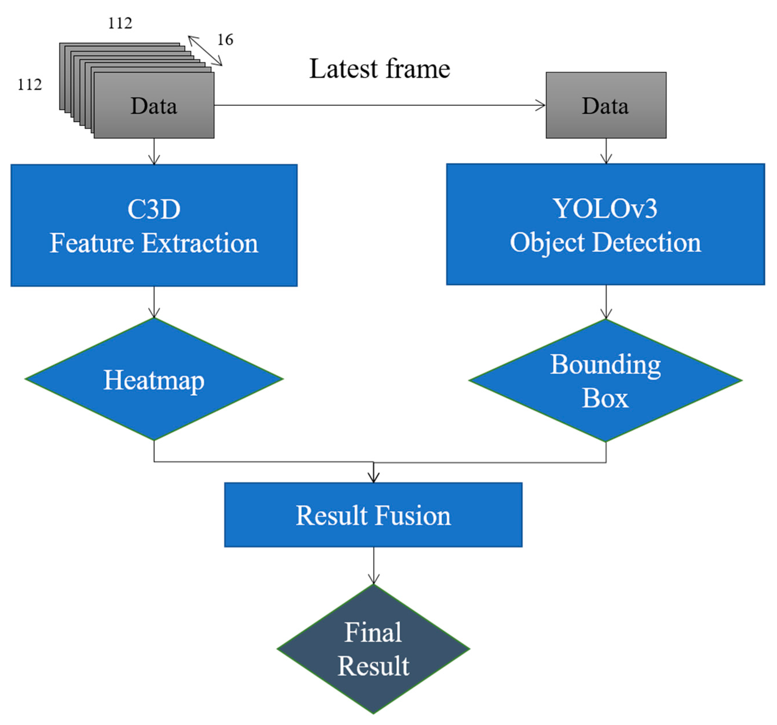
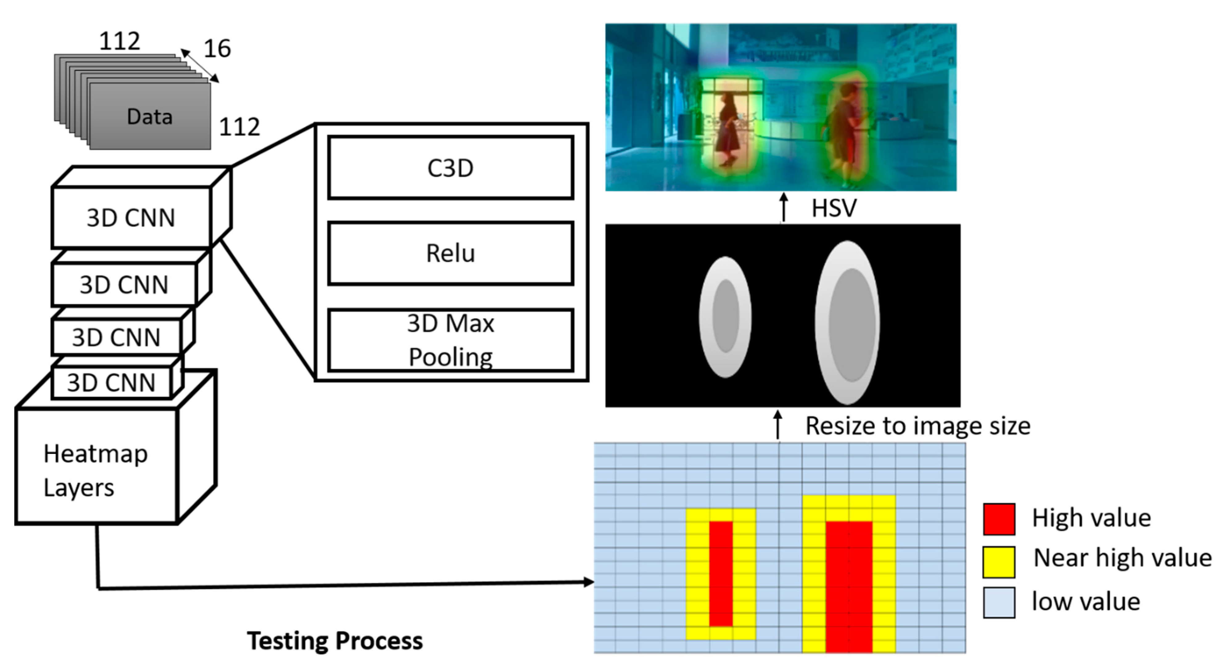
Figure 4 shows the overall architecture employed in this literature. The detected results from the YOLO v3 object detection model is fused with those from the C3D model to improvise the stability as well as accuracy of the behavioral heatmap. The following sections detail the steps involved in the behavioral prediction method.
3.1. Architecture of the Proposed C3D Feature Extraction Model
The C3D CNNs are faster than the CNN models with recurrent operations. However, the 3D convolution imminently requires more computational time and require more parameters.
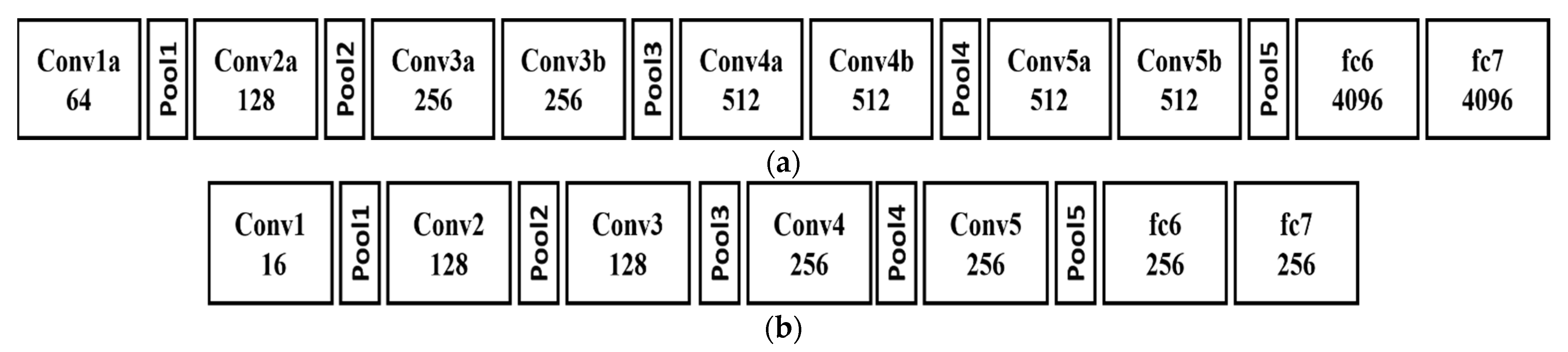
The original C3D CNN architecture commonly comprises of eight 3D convolution layers, five 3D pooling layers, and two fully-connected layers, as depicted in
Figure 5a. It is comparatively faster than those with recurrent positions. Despite the fact that the NN is very shallow, it is still large and too slow to be implemented in embedded systems for real-time applications.
The conventional C3D NN designed for UCF101 contains 101 human behavior classes. While implying it for ADAS applications, it is not needed to perform meticulous judgement. Therefore, this paper simplifies the conventional C3D architecture to only possess five 3D convolutional layers, five 3D pooling layers, and two fully connected layers, as exhibited in
Figure 5b. The output channel size of every 3D convolution layer and fully connected layer are far lesser than the conventional C3D. With this simplification [
24], the model is faster and requires comparatively lesser parameters and lower computational cost. Thus, the simplified C3D model proposed in this paper is represented as in Equation (1), where
H represents the output behavior heatmap,
f is the C3D function,
x is the image sequence, and the subscript
t−15:
t implies that the input depth of C3D model is 16 frames.
Additionally, the proposed model is a combination of C3D and YOLO v3 object detection model in which the detected objects are considered as behavior candidates and the C3D model determines whether the considered behaviors are in the bounding boxes. Thus, the proposed fusion architecture can be represented as in Equation (2).
3.2. Pre-Trained Model of the C3D
The key objective of the pre-trained model [
25] is to perform behavioral recognition. The pre-trained deep learning models provide enhanced performance without any additional costs. The challenge of object classification and detection has not only a large amount of pre-trained models but also diversified models, whereas the pre-trained models for behavioral prediction are negligible and limited to certain specific situations. Since the behavioral definition targeted in this paper is dissimilar to the definition of common behaviors, the improvements that standard publicly available action/behavior recognition datasets contribute is scarcer. In order to gain an improved performance, the authors have created a pre-trained model themselves. The data to train the pre-trained model is obtained from the identical datasets used for behavior prediction, but with a different approach. In a video clip used as an input, the pre-trained model should be capable of determining if the video clip has any pedestrian(s) crossing, vehicle(s) cutting-in, and vehicles applying sudden brakes or slowing down ahead.
A dissimilar set of frames are categorized according to pedestrians and vehicles followed by dividing each video into a large amount of video clips consisting of 16 frames, termed as ‘input data’. Only those video clips that include pedestrians and pedestrian(s) crossing the road is considered as ‘true’ input ground truth. Similarly, behaviors such as vehicles cutting-in and vehicles applying emergency brakes are defined. According to this definition of ‘behavior’, the pre-trained model used in the paper learns better and more accurate features of the behaviors of pedestrians and vehicles.
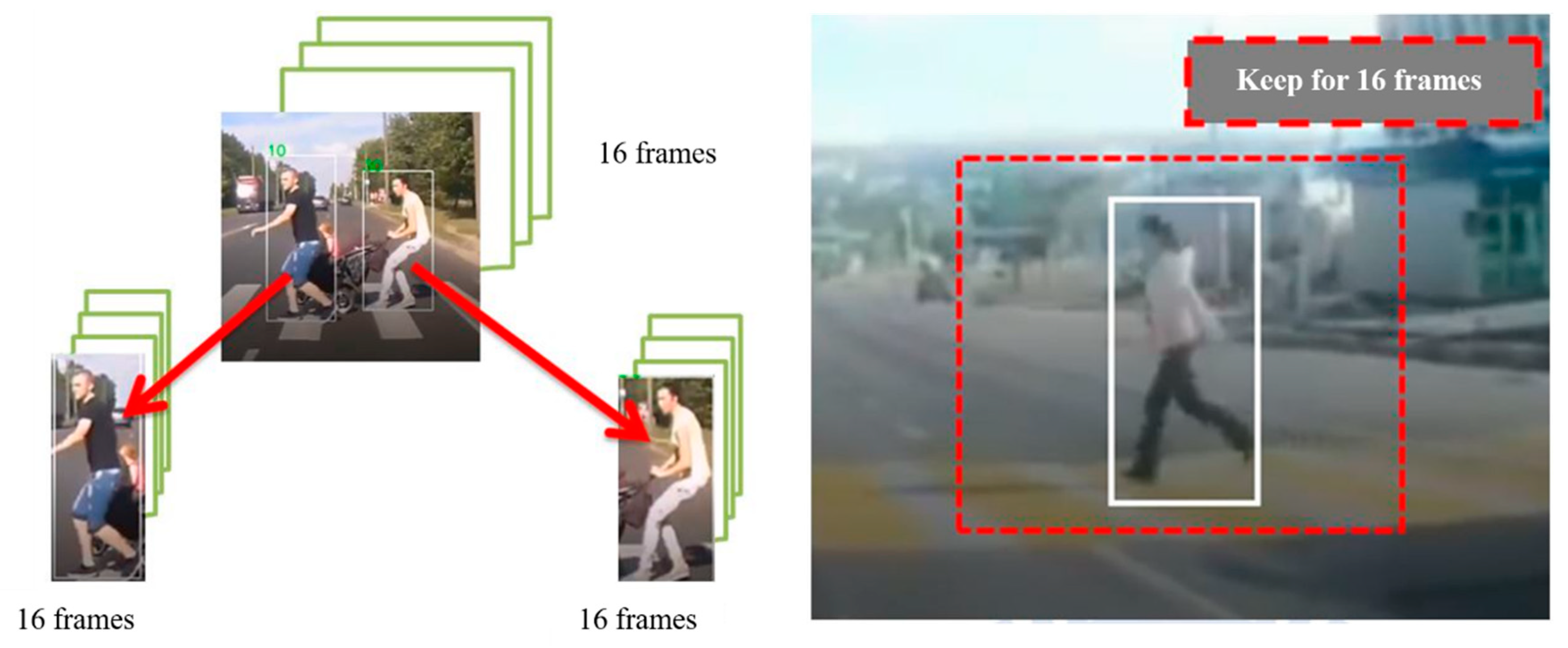
In order to enable the pre-trained model to assimilate information about pedestrians crossing, vehicles cutting-in and vehicles applying emergency brakes, the snipped region of the input video clips is adjusted to retain the motion information of the pre-trained model. If the focus is set only on pedestrians and/or vehicles and allows the pedestrians and vehicles to be located in the center region in every frame of the clip, it may cause loss of motion information, resulting in reduced efficiency. The crop box bigger than the bounding boxes of pedestrians is set, as represented in
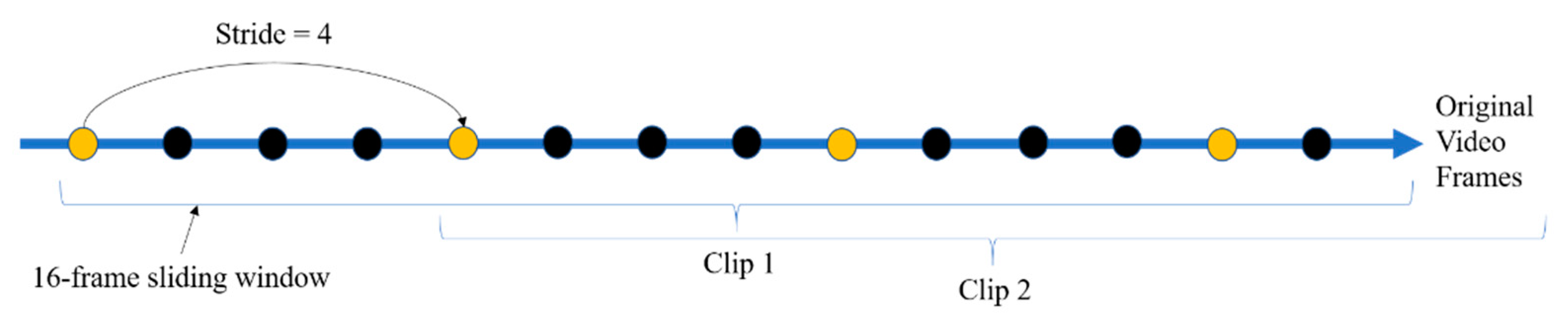
Figure 6, and cropping boxes are allowed to move every 16 frames. That is, the input video clips comprise of the crossing motion of the pedestrians, causing preferential improvement with the pre-trained model. Furthermore, in order to increase behavioral prediction efficiency, this paper attempts different strides for the 16-frame sliding window to extract training clips from the videos, as represented in
Figure 7. The yellow/black circles on the arrow are the frames in the original videos. The videos are then pre-processed into many 16-frame clips for training, so a parameter called a ‘stride’ is set to adjust the frame-overlapping rate of adjacent training clips, as shown in
Figure 7.
3.3. Depth-Wise C3D Model
In order to process the C3D model on embedded systems, it is a necessary pre-requisite to reduce the number of parameters. Therefore, a depth-wise 3D convolution is applied. Since the depth-wise 3D convolution [
34] has an impressively reduced number of parameters, this paper uses it to perform parameter reduction. The comparison of the parameters of the simplified C3D model without a heatmap layer using the original 3D convolution with that of a depth-wise 3D convolution is as shown in
Table 1.
3.4. 3D Convolution Neural Network with a Heatmap Layer
When predicting the behavior of pedestrians, vehicles cutting-in, and vehicles applying brakes for ADAS applications, as the objects are not always in the middle of the real-time environment scenes while driving, the two challenges to be considered are: (i) to ascertain the position of target objects and (ii) to categorize the behavior of the target object. However, the two-stage behavior prediction also has certain hurdles, such as, (i) to ensure the accuracy and stability of object detection; (ii) to support behavior recognition, the object detection results must be stable. Otherwise, the behavior recognition that results in unstable or even wrong input source from object detection is nearly impossible to output correct behavior; and (iii) computation time cost—since we are required to complete the two models, object detection and behavior prediction, topologically, it unpreventably costs more time.
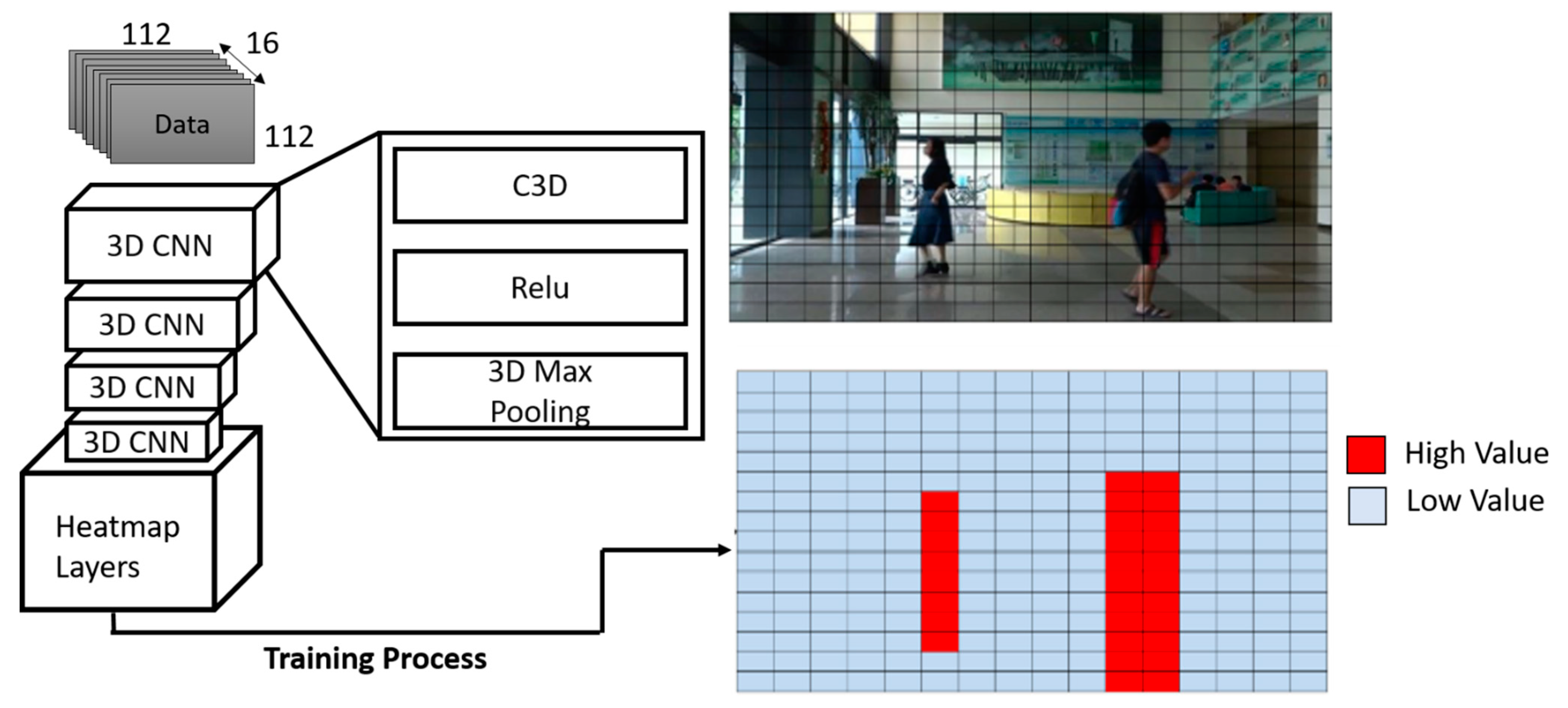
In order to tackle the previously mentioned challenges, the concept of harnessing a heatmap layer is attainable and considered ideal as the heatmap layer, besides containing spatial features, also contains temporal features. The heatmap layer is included after the C3D feature extraction. During training, a 16 × 16 feature map is created by the model proposed in this paper. The original image, which is the last frame of the input video clip, is disjoined into 16 × 16 grid maps to correspond to 16 × 16 output feature maps. The grid that has the targeted behavior is represented by a higher value, whereas the other grids are set to lower values as in
Figure 8.
During the testing process, each grid in the 16 × 16 grid maps is designated a value from the proposed algorithm. If the target behavior appears at the location of one of the grids, the value of that is considered to be nearer to the higher value; otherwise the value is weighed closer to a lower value. After obtaining a 16 × 16 grid map, it is enlarged into a gray scale intensity map equivalent to the size of an image, followed by modification of an intensity map into a HSV picture termed as heatmap. In the heatmap, the region with a higher value is depicted in red, while the region with lower value is in blue, as in
Figure 9. In the end, the heatmap is overlaid onto the original source picture so that the locations of the target behavior are clearly present as it occurred.
Two different ways can be adapted as a means to obtain the final heatmap results following C3D feature extraction namely: (i) to use a fully-connected layer; and (ii) to use un-pooling layer and 3D convolution. Both these ways have similar accuracy and speed, where there are notable differences in the required number of parameters as discussed in
Section 3.4.1.
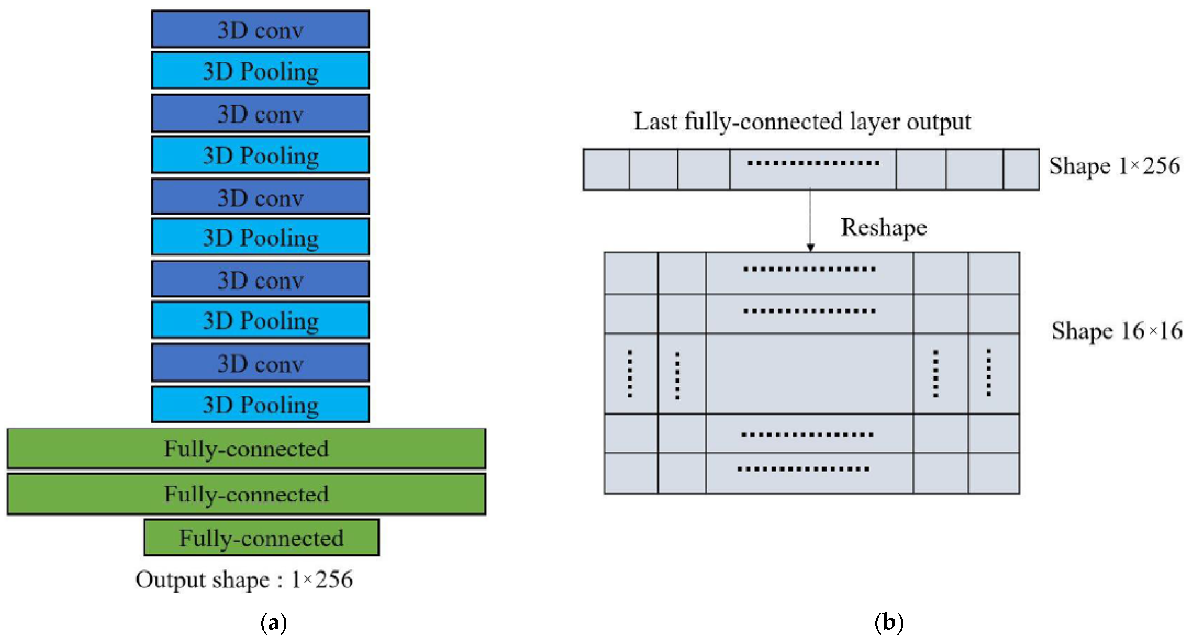
3.4.1. Heatmap Layer Using Fully-Connected Layer
The total architecture of behavioral prediction with a heatmap layer using fully-connected layer is as shown as
Figure 10a. The architecture uses three fully-connected layers to produce a 1 × 256 flattened intensity vector. Similar to traditional C3D networks, the numerous fully-connected layers following the feature extraction of 3D convolution are used to compress the information of the features so that the final classification can be carried out.
The previous two fully-connected layers are also utilized for information compression. In the final fully-connected layer, it is necessary to adjust the length of output intensity vector of size 1 × 256 so that the intensity vector length is the square of that of the heatmap size, as in
Figure 10b. In this paper, the intensity vector transform is reshaped into an intensity heatmap.
3.4.2. Heatmap Layer Using an Unpooling Layer
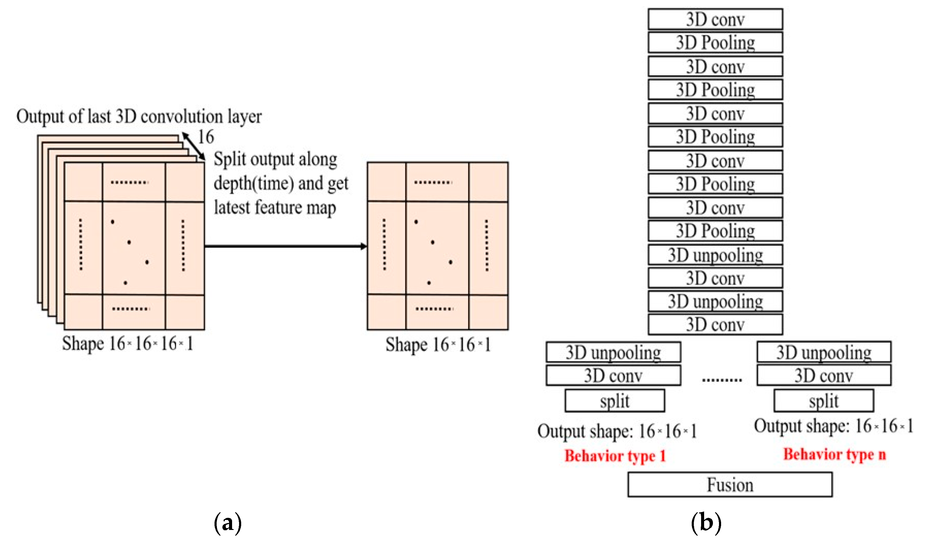
In order to obtain the end results of heatmap following C3D feature extraction, we adopted an unpooling layer and 3D convolution. The concept of employing an unpooling layer is influenced by the SegNet [
34]. After numerous 3D convolutions and 3D pooling layers, the unpooling and 3D convolution is used to inflate the feature map to a desired output shape.
The output features possess width (W), height (H), depth (D), and channel (C) size of 16 × 16 × 16 × 1, respectively, after the final 3D convolution layer. The channel size is 1, considering it is merely an intensity map. Because the dimensional length of input depth is 16, the output can be viewed as a combination of heatmap respective to every frame of the input video clip. Therefore, the dimension of 16 × 16 × 16 × 1 is split along the depth dimension to achieve an output with dimension 16 × 16 × 1 × 1 intensity heatmap, as in
Figure 11a.
In order to determine the behaviors of multiple object, the architecture of the heatmap layer is experimentally adjusted. By utilizing different heatmap layers to correspond to different behaviors, a model competent to detect the behaviors of various objects simultaneously is trained, as in
Figure 11b. The model size and computation cost is expected to rise with more behaviors for recognition, which is practically acceptable in case of real-time applications.
By performing unpooling, the output maintains the shape of 3D features so that both spatial and temporal domain information are maintained well. Further, a large number of input and output channels result in a huge number of parameters of fully-connected layers. On the other hand, there are barely any parameters for unpooling layers. Thus, only the 3D convolution layers need to calculate the number of parameters and it is lesser than using fully-connected layers, as in
Table 2.
3.5. Dataset for Multi-Object Multi-Behavior Prediction
For prediction of real-time behaviors, the crucial step is to carefully describe the behaviors. The prediction of behaviors in real time is completely different from commonly followed off-line behavior recognition. A majority of publicly available standard behavior datasets customarily focuses on common human activities, such as walking, running, and standing, among others. Therefore, the behavior analysis for drivers of motor vehicles is not supported by these datasets and public behavior datasets that are used for video recognition usually take the whole videos and then recognizes the behavior. However, it is mandatory to analyze the behavior instantaneously and alert or at least inform the driver in real time. Therefore, the behavior should be defined carefully and clearly so that it can be determined in every single video clip used during testing.
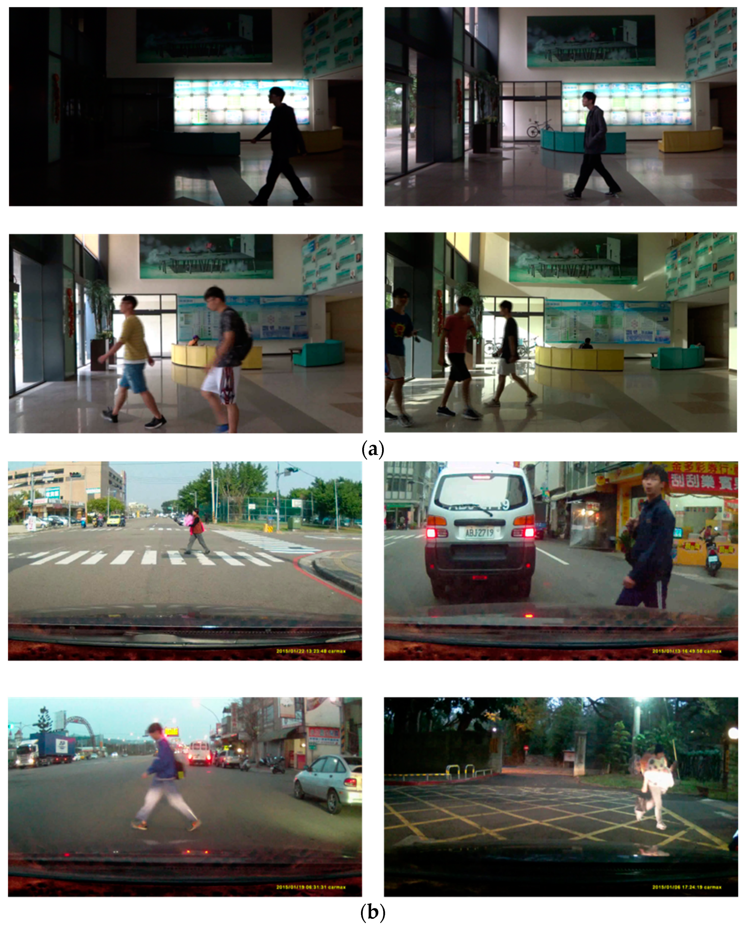
The human activities and vehicular recognition datasets assume that the target is in the middle of a scene while the targets in real environments may appear in different corners and sometimes just in a small part of the scene. In order to overcome these drawbacks, this paper collected pedestrian crossing dataset from a fixed indoor camera, as well as from a car camcorder, as shown in
Figure 12a,b, respectively. Similarly, vehicles cutting-in and vehicles applying brakes dataset are built using videos from car camcorders.
The datasets thus built are further labelled with targeted objects in bounding boxes and corresponding behaviors of the respective objects in motion through individual colored heatmap such as Yellow: pedestrian crossing, Blue: vehicle cut-in, Purple: emergency brake (
Figure 13).
The distribution of training clips with different strides, as mentioned in
Section 3.2, along with basic data augmentation methods such blur, noise, and flip, are as given in
Table 3. For each behavior, we collected about 100 short videos in different environments varying from peak hours to non-peak hours and from daytime to nighttime. Of these 100 videos, approximately 95 videos are used for training and the remaining 5 are used for testing. The length of each video is about 3~5 s. For training, we employed 3 different clip strides to divide the 95 short videos into training clips, as listed in
Table 3 and Table 8. Then, the remaining five videos of each behavior are used during testing.
Table 4 shows the distribution of the testing clips.
3.6. Loss Function and Accuracy of Heatmap Layers
Since the heatmap is different from action recognition, only loss function and accuracy calculation cannot be used. Therefore, the authors in this paper designed a loss function and have their own definition of accuracy.
The loss function of the traditional C3D uses the softmax cross entropy, which is widely used for image and action recognition applications. However, the softmax cross entropy can be used only when the output is a “class” of a data. For heatmap, an intensity map acts as the output. In every grid, an amount value is available, instead of a class. Since the heatmap’s intensity map has spatial relation, the heatmap is finally overlaid on an original image followed by the application of the loss function called ‘Euclidean loss’. The Euclidean loss is a loss that adopts the concept of Euclidean distance. It calculates distance in Euclidean space, which is to calculate the similarity of two lines. Like some models for image processing, the Euclidean loss is utilized to calculate the difference between the output and the ground truth. Thus, when calculating loss, the output and ground truth are first flattened and then the Euclidean distance of these two as loss is calculated and used to train the model.
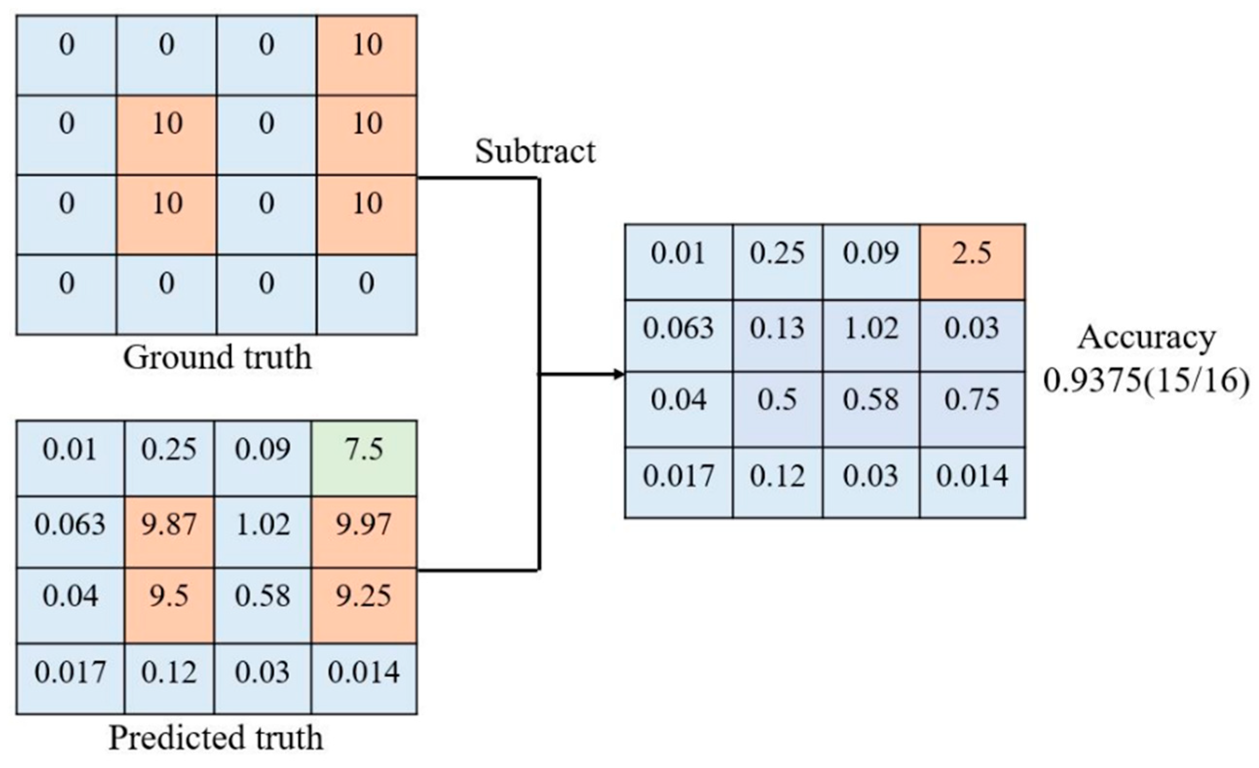
The accuracy of a heatmap is calculated in three steps. (i) First, the accuracy of a single frame heatmap is calculated. For a single frame, there will be one heatmap with 16 × 16 grid. The predicted result value and ground truth-value are then subtracted, as shown in
Figure 14. (ii) After the subtraction, only the grid with an absolute value less than that of the experimentally set threshold value is considered as correct. There are three threshold values individually corresponding to ∆, ∆
2, and ∆
3 accuracies, as tabulated in
Table 5. The default setting of the threshold value in this paper is 1.5, which is experimentally chosen. Then, the number of correct grids are counted and divided by total grid numbers to get frame accuracy. For accuracy of a video, all of the frame accuracies, excluding the first 15 frames, are calculated and the average of all the frame accuracies is considered as the whole video accuracy. (iii) Finally, the average of all the test video accuracies is taken as the overall total accuracy.
3.7. Object Detection Using YOLO v3
Along with the proposed C3D model detecting the behavior of pedestrians, vehicle cutting-in, and vehicles applying emergency brakes, YOLO (You Only Look Once) v3 is employed to detect the objects. YOLO v3 uses the pre-trained model of C3D discussed in
Section 2, along with the bounding boxes, to perform object detection in unseen scenes of real-time environments for ADAS applications and to output a model. The output model is then fused with the results of the C3D model. The method of fusing the results of the YOLO v3 object detection model with that of the results from the proposed C3D model is discussed in
Section 4.
4. Experimental Results
This section presents the implementation details and results of the proposed multi-behavior detection method.
The proposed C3D heatmap algorithm is exploited on a server with NVIDIA GTX1080Ti. Both the training and testing are done on this server. In order to explore the compatibility of the proposed method for our targeted real-time applications of ADAS, NVIDIA Jetson AGX Xavier is used as the embedded platform. The NVIDIA Jetson AGX Xavier adopts a Linux environment and supports many common APIs. It is also supported by NVIDIA’s complete development tool chain and has a variety of standard hardware interfaces that make the platform highly flexible and extensible. Due to these reasons, the NVIDIA Jetson AGX Xavier is considered ideal for the proposed application requiring high computational performance with low power requirements.
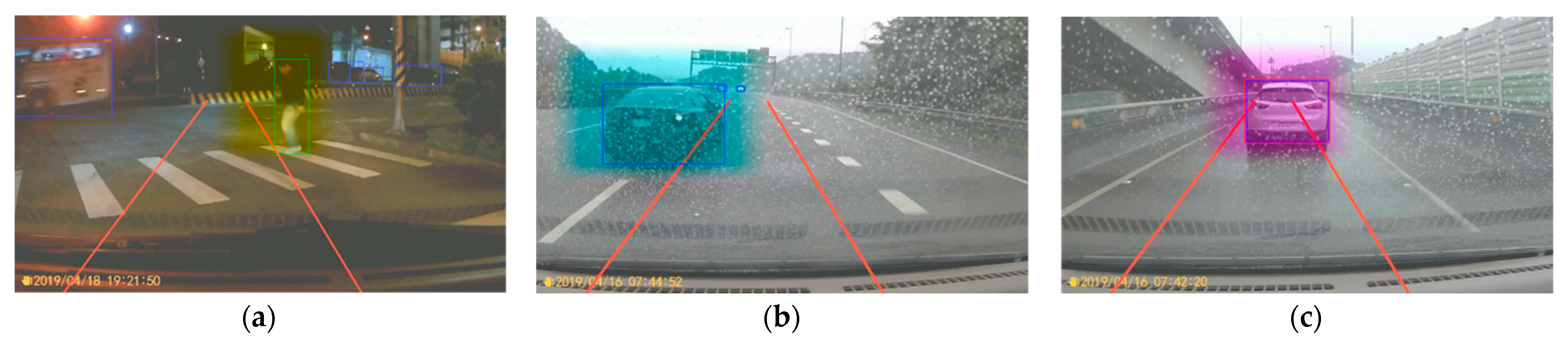
With the result of heatmap, it is possible to predict the tentative location of the targeted behavior of moving objects. Then, with the YOLO v3 object detection result, the precise position of the object is detected. After combining these two results, a noise-free heatmap is obtained.
For emergency brake detection, a ROI is set to make the system focus on front vehicles. A vehicle is taken as an emergency brake candidate if the middle-bottom point of its bounding box is in the ROI. The corresponding color of bounding boxes for respective behavior are as listed in
Table 6 and the heatmap color if the detected candidate has such behavior is as in
Table 7. The results from the proposed method of heatmap pedestrians crossing, vehicle cutting-in and vehicle applying emergency brakes are as shown in
Figure 15. Further, the results with respective color-coding for different object behaviors are as shown in
Figure 16. Here, yellow represents pedestrians crossing, blue represents vehicles cutting-in, and purple represents vehicles applying emergency brakes.
Table 8 shows the experimental results depicting the impact of different strides setting for training clips on testing accuracies on the NVIDIA GTX 1080Ti. Finally, the version trained with training clip stride 4 is chosen in the proposed method. The number of parameters required for the C3D model to predict these three behaviors are 5.97 M and the overall speed of this system on GTX 1080Ti is 40 ms processing at the rate of 25 fps.
5. Discussion
The state-of-the-art of methods such as [
12,
20,
21,
22,
23,
24,
25,
26,
27,
28,
29,
30] and others are evaluated with a single resolution of input videos and for the detection of single behavior at a time, whereas the proposed method is tested for different resolutions of input videos and multiple behavior detections, as we know that videos with better resolution provide more information. However, since the input scales up from images to video clips, it becomes more difficult to deal with the input. With the increasing size of input video clips, the computational cost, number of parameters required, and FPS (frames per second) have significant impacts on the performance of the NNs. The comparison of input video clips of sizes 112 × 112 × 16 and 224 × 224 × 16 using the original C3D with a fully-connected layer as heatmap layer are listed in
Table 9.
As seen in
Table 10, the input video of size 224 × 224 requires more number of parameters and results in slower computational speed. On the other hand, there is no significant improvement in accuracy when the size of the input clip size changes from 112 × 112 to 224 × 224. Since a pedestrian is a small object compared to the original 1920 × 1080 input size, two times the input size may not have a greater impact in enhancing the accuracy of the behavior analysis.
Additionally, most previous papers lack an attempt to decrease model size, reduce the number of required parameters or both, leading to the design of a model compatible with embedded system implementations suitable for practical ADAS applications. Unlike previous papers, this paper covered an evaluation of the impact on accuracy with decreased model size and number of parameters, as tabulated in
Table 10. The conventional model C3D model, C3D_v1, and the lightweight model, C3D_v2 to C3D_v6 with different channel sizes proposed in this paper, are compared as tabulated in
Table 10. The original model possesses the model channel size employed in the C3D and the lightweight model contains the channel size, as discussed in
Section 3.3. As estimated, the decrease in model size resulted in the reduction of accuracies. However, compared to the reduction of accuracies, it has resulted in the betterment of FPS and also reduced the required numbers of parameters, as listed in
Table 11.
To decrease the parameters and computational time of the proposed model, the channel size of each layer is adjusted. The comparison of different C3D models with distinct channel sizes in each layer are listed in
Table 10. To make the proposed model faster enough to suit real-time applications, the C3D_v1 model is excluded from real-time applications because of its low speed. Among the other models with acceptable speed, the C3D_v3 model is more appropriate for real-time applications as its accuracy is the highest of all models.
To make the proposed model predict more accurately, a pre-trained model, as mentioned in
Section 3.2, is employed. Although many state-of-the-art methods [
12,
20,
21,
22,
23,
24] have employed the pre-trained model for their respective implementations, these papers have failed to evaluate how it alters the accuracy of the model. This paper compares the proposed model with and without a pre-trained model (
Table 12) and thus analyses the influence of the pre-trained models. All the basic models of behavior prediction are the lightweight C3D model.
As shown in
Table 12, the pre-trained model has resulted in a small improvement in accuracy with the input clips of both sizes. The improvement can even make the lightweight model better than the original model without increasing of number of parameters and decreases FPS.
The crucial part of the proposed method is the heatmap layer, which is not employed in previous papers. This paper evaluates two different types of heatmaps, as discussed in
Section 3.4. Of the two types of heatmap layers, as mentioned in
Section 3.4.1 and
Section 3.4.2, respectively, the unpooling heatmap layer is better than the fully connected heatmap layer, as represented in
Table 13—it shows a comparison of these two kinds of heatmap layers, showing experimental results. Both the models are tested using the lightweight model.
From
Table 13, it can be noted that the heatmap with unpooling layer achieves an impressive improvement in accuracy and at the same time, has no drop in FPS. The unpooling heatmap also has good performance in reducing the numbers of parameters, as compared to the fully connected heatmap.
The final comparison is the depth-wise 3D convolution, as shown in
Table 14. A depth-wise network can be obtained by replacing all the traditional convolution layers with a depth-wise 3D convolution layers.
Table 14 shows the comparison of the proposed depth-wise C3D model with those of the original 3D convolution models.
As seen from
Table 14, the depth-wise 3D convolution incredibly decreases the number of parameters. The unpooling heatmap layer model has more reduction than the fully-connected model with increased accuracy. However, the proposed depth-wise 3D convolution does not have any parallel processing or accelerating methods. Therefore, a decrease in the speed of depth-wise 3D convolution can be noted, compared to the original 3D convolution. Additionally, although the depth-wise C3D convolution has far lesser parameters, NVIDIA Jetson Xavier cannot achieve its efficient implementation and even TensorFlow (TF) [
35] does not support it. Thus, the depth-wise C3D is not considered in the final implementation in this paper.
Table 15 shows a comparison of the efficiency of the single and mixed behavior models. These use lightweight models and are without the pre-train models. It can be noted that the multi-behavior models achieve similar accuracies for detecting multiple behaviors with a slightly increased computation cost.
6. Conclusions
This paper proposes a lightweight 3D convolution model with heatmap layers using fully-connected layers and unpooling layers to detect pedestrians crossing, vehicles cutting-in, and vehicles applying emergency brakes. The heatmap layers for identifying objects in real traffic environments based on their behaviors is evaluated and it appears to be fruitful in yielding enhanced accuracies for detection of multiple behaviors simultaneously. The proposed design is optimized for computational low complexity and to possess a smaller model size, as low as 5.7 MB, to be convenient enough to realize in embedded systems like NVIDIA Jetson Xavier, which most state-of-the-art methods lack in respect to multiple object detection in real-time for ADAS applications. The proposed method achieved 10 frames per second when deployed on NVIDIA Jetson AGX Xavier and yielded over 92.8% accuracy for pedestrians crossing, 94.3% accuracy for vehicles cutting-in behavior detection, and over 95% accuracy in recognizing vehicles applying emergency brakes or abruptly slowing down ahead. Based on factual consideration that for vehicles traveling on freeways/highways, there will not be any pedestrians whereas in urban areas vehicular speed is under 50–60 kmph, the processing speed of 10 fps is considered adequate. Compared to most deep learning object detection models, the proposed design further supports multiple behavior recognition for targeted moving objects, like pedestrians crossing, vehicles cutting-in, and vehicles applying emergency brakes, which is beneficial to ensure safety in ADAS systems, thus aiding in the prevention of potential accidental dangers. Furthermore, the pre-trained models affected the efficiency of the proposed method in a positive manner, resulting in enhanced accuracy compared to those without pre-training. Although many of the previous object detection methods have employed pre-trained models, they were all for single object detection and single behavior detection, unlike in this paper. We are skeptical that the pre-trained model will have any repercussions, although the chances cannot be completely denied. We will attempt to explore the potential repercussions in future extensions of the proposed algorithm. In other words, there are some false predictions in outdoor testing data and there are certain behaviors such as bikes, scooters, mini trucks, trucks, and buses cutting-in and applying emergency brakes, along with wheelchair pedestrians, children, and stray animals, which are not included in the present literature. This proposed algorithm is being extended to support broader aforementioned behavior analysis applications in the future and make it a crucial part of the ADAS system effective in enhancing the safety of passengers, pedestrians, and properties.


