Measuring the Realtime Capability of Parallel-Discrete-Event-Simulations

Abstract

Speeding up Discrete Event Simulations (DESs) is a broad research field. Promising Parallel Discrete Event Simulation (PDES) approaches with optimistic and conservative synchronisation schemes have emerged throughout the years. However, in the area of real-time simulation, PDESs are rarely considered. This is caused by the complex problem of fitting parallel executed DES models to a real-time clock. Hence, this paper gives an extensive review of existing conservative and optimistic synchronisation schemes for PDESs. It introduces a metric to compare their real-time capabilities to determine whether they can be used for soft or firm real-time simulation. Examples are given on how to apply this metric to evaluate PDESs using synthetic and real-world examples. The results of the investigation reveal that no final answer can be given if PDESs can be used for soft or firm real-time simulation as they are. However, boundary conditions were defined, which allow a use-case specific evaluation of the real-time capabilities of a certain parallel executed DES. Using this in-depth knowledge and can lead to predictability of the real-time behaviour of a simulation run.

1. Introduction

Discrete Event Simulations (DESs) are used to model systems that cannot be described with continuous simulation [1]. In contrast to continuous models, DES change their internal simulation states only in response to events bound to specific timestamps. Simulation frameworks like OMNeT++ (https://omnetpp.org/ (accessed on 15 December 2020)) can be used to model any event discrete system without being restricted to a certain domain. Other simulators are bound to specific domains like NS-3 (https://www.nsnam.org/ (accessed on 15 December 2020)), which is dedicated to computer networks. DESs frameworks provide an environment that is used for the development of simulation models which cover the domain-specific properties of a certain system to simulate.

When speaking of DES, traditionally, their simulation models are executed in a single-threaded fashion. According to Fujimoto [2], this simplifies the event scheduling, as a single-threaded simulation is a closed system without stimuli from other execution contexts. However, the growing complexity of simulation models is consuming the calculation capacity of one computing core to the fullest. This results in very limited execution speed for certain models. Especially, in the area modelling large wireless networks with high node mobility, the scenario complexity is restricted due to the vast time consumption of a simulation run.

At first glance, this might not be a severe problem. Waiting for a week until a simulation of two or three simulated real-world seconds has finished might just be tiring, but it is not affecting simulation results. However, certain use cases require simulations to interact with real hardware. In this case, slow-paced execution speed of a simulation is affecting their results. Closed-loop Hardware in the Loop (HIL) testbeds are a perfect example for simulation systems, demanding real-time execution speed. Even though more capable hardware could be used, many existing models still exceed the power of a single core to be real-time capable.

Vehicular Ad Hoc Network (VANET) simulators like presented by Hegde and Festag [3] are such a calculation-intensive domain when complex scenarios are computed. VANETs are networks which are established between several participants in road traffic [4]. These can be, among others, cars, motorcycles, trucks or roadside units. Realistic vehicle mobility is required to evaluate the network behaviour properly. Thus, coupling the network simulation with a vehicle traffic simulator is advisable, as as described by Sommer et al. [5]. Research on VANET performance, that is, channel congestion and packet routing, demands for a high number of communicating vehicles. For this reason, city-scale scenarios like the Luxembourg scenario presented by Codeca et al. [6] are required. This leads to a significant lack of simulation speed, like shown by Obermaier et al. [7]. Hence, several research groups already tackled the problem of speeding up DES in general by developing strategies for executing them on several cores. However, none of these approaches consider real-time simulation.

As Parallel Discrete Event Simulations (PDESs) aim for increasing the overall simulation speed, use cases that require simulations to be carried out in real time might also benefit from these ideas. However, according to literature, PDES were not designed with real-time execution in mind. Thus, this paper proposes a metric that allows for ranking parallel executed DES with respect to their real-time behaviour regardless of the employed synchronisation strategy. This metric can be used to further investigate the question if PDESs are possible in general for simulations running in real-time. However, rankings discovered using the metric cannot be transferred easily between modelling frameworks and synchronisation strategies. This is caused by the fact that modelling paradigms have a significant impact on the results of a simulation model.

Evaluation of the timing behaviour of a HIL system is mandatory when it comes to execution of realistic test cases. However, this is often neglected in current literature. For example the Vehicle-to-Everything (V2X) communication simulator developed by Zhang and Masoud [8] states to have an adapter to integrate real-world hardware to facilitate HIL tests. However, they do not evaluate their system with respect to actual timing. Similarly, Menarini et al. [9] present a dedicated V2X HIL framework without further insights of the timing behaviour. Thus, this paper presents a solution how such a real-time analysis can performed without being bound to any specific simulation system or simulator. To do so, a metric is presented, allowing to compare different simulators with respect to their real-time behaviour. Moreover, the metric is designed to be suitable for any kind of DES simulator, independent if they are executed on one or several cores.

This paper is organized as follows: Section 2 revisits the definition of a DES. Also, principles of real-time simulation are presented. In Section 3, a vast overview of PDES architectures found in literature is shown. Section 4 introduces the metric to analyse the real-time capabilities of a simulation run. A demonstration, how this metric can be applied, is detailed in Section 5. Section 6 shows which requirements must be fullfilled by a simulation framework for the metric to be applicable. It is also presents boundary conditions and how they correlate to the outcome of the metric. Section 7 concludes the paper and outlines future work.

2. Time in Discrete Event Simulations

DESs are often used to model systems that cannot be depicted using continuous simulation systems. Common use case are simulations of computer networks or other complex connected systems [10]. Thus, DES frameworks share a common aim—providing a framework that abstracts from a particular simulation model as much as possible to untie a simulator from specific domains.

2.1. Real-Time Systems

Before discussing how time affects a DES, the overall concept of real-time systems must be revisited. The main feature of a real-time system are deadlines which the system has to meet reliably when executing tasks [11]. Meeting deadlines means that the real-time system must be able to observe when tasks finish. Moreover, the system has to report if the required deadline was violated or avoid violating them completely. According to Laplante and Ovaska [12] and Erciyes [11], real-time systems can be divided into three categories, each of them with their own features and requirements:

• Soft real time is the weakest category of systems executed in a real-time manner. In this category, missing a soft deadline is allowed and not critical at all. However, the overall system’s gain degrades depending on the amount of missed deadlines [11,12]. An example of such a system would be a multimedia stream, whose quality lowers when certain frames do not arrive in time.
• Firm real-time systems describe systems which are not allowed to miss a single deadline. Their gain immediately degrades to zero, when one deadline is missed. However, no fatal injuries or high costs are caused by such a missed deadline [11,12]. VANET HIL testbeds are examples for firm real-time systems: No injuries are caused when the testbed misses its deadlines but the test run looses all its significance.
• Hard real time is the strongest category of real time. Missing a hard deadline can cause catastrophic results, which means special hardware and software is required to ensure that each and every is met [11,12]. Examples for such systems can be found in many disciplines, like airbag Electronic Control Units (ECUs) or aircraft manoeuvring systems.

Soft and firm real-time systems can be implemented without the need of special hard- or software. It is sufficient for the system to watch the set deadlines and report violations or apply recovery strategies upon violation. For hard real-time systems, however, guaranteeing deadlines is mandatory. Thus, hard- and software need to be able to enforce execution of tasks within a certain time span. For example, real-time operating systems like Linux systems with real-time extensions or dedicated microcontrollers can guarantee this strict timing.

Commonly, DESs are running on commodity hardware without real-time features in place. This means that it is not possible for them to meet hard real-time requirements. Thus, this paper focuses on soft and firm real time, as this is achievable with off-the-shelf DESs like OMNeT++. In the following, this paper refers to soft and firm real time, except where hard real time is explicitly mentioned.

2.2. Discrete Event Simulations

In contrast to continuous simulation, DESs do not assume a uniform flow of time. Whereas a continuous simulation is in a permanent state of flux, state changes in discrete event models happen only at specific points in time [13]. These time points are bound to certain events, as shown in Figure 1. The simulated time jumps from event to event as the time between events can be skipped entirely [14]. Between events, the simulation state is fixed.

Events are stored in a so-called Future Event Set (FES). The FES can be seen as a list of all already known future events. At the very beginning of a simulation, at least one event has to be scheduled in the FES, as an empty FES indicates a finished simulation run. This initial event usually generates subsequent events which are scheduled at future time points. However, events do not need to be generated in a timely ordered manner. For example, the events shown in Figure 1 could occur this way: The initial event is the green event scheduled at time point 0. This event is subsequently creating the blue and the yellow event bound to the time points 5 and 20, respectively. At time point 5, the blue event is creating the orange event, which is tied to time point 9, and therefore, has to be executed before the yellow event is executed. Thus, the internal event scheduler has to take care of establishing a correct timeline by executing the events in chronological order. This is required to ensure that no causal dependencies of events are violated. Hence, to ensure deterministic event processing, the scheduler takes care of maintaining an ascending simulation time. During event execution, it is also possible to cancel already scheduled events. However, this event’s timestamp has to be in the simulated future [10].

As already mentioned, the time in a DES is not bound to any continuous wall-clock or Central Processing Unit (CPU) time. Hence, the current simulation time has to be stored in a variable. During the main simulation loop, which is processing event after event, this variable will be updated at the beginning of each event. Thus, when requesting the current simulation time during the execution of a single event, the simulated time will not change, independent of the CPU time needed to execute the event. Even more, it is common that an FES might contain events which are scheduled at the exact same timestamp. Even though the sequential execution of these events might take quite a high amount of CPU time, the simulation time remains the same for all events scheduled at the same time [10].

2.2.1. Formal Description of DES

A detailed formal description of a basic DES system M can be found in [15]:

$$M=\langle X,S,Y,{\delta }_{int},{\delta }_{ext},\lambda ,ta\rangle ,$$

(1)

where X is the set of input values, S the set of states and Y is the set of output values.

• ${\delta }_{int}$ is the internal state transition function ${\delta }_{int}:S\to S$.
• ${\delta }_{ext}$ is the external transition function ${\delta }_{ext}:Q\times X\to S$ where $Q=\left\{\right(s,e\left)\right|s\in S$, $0\le e\le ta\left(s\right)\}$ is the total state set and e the elapsed time since the last event.
• $\lambda$ describes the output function $\lambda :S\to Y$.
• $ta$ is the time a system stays in a state s with the mapping $ta:S\to R_{0,inf}^{+}$.

At the beginning of a simulation run, the whole system with all its components is in a specific state s. This state is defined by, among others, the given input values x. As no state changes occur without events, the next state change can be predicted by $ta\left(s\right)$ when looking at the next scheduled event in the FES. Zeigler et al. [15] divide events into internal and external events. Whilst the next internal event is always known by a simulated system (as it schedules this internal event for itself), external events maybe not always known. Hence, when an external event changes the state s to a state $s^{\prime }$, internal events might be cancelled or changed.

2.2.2. DES with Several Connected Components

Usually, a DES does not only consist of one component, like specified in Equation (1). Modelling a whole system as one component is more complex than breaking the system down into several sub-components. Thus, Zeigler et al. [1] extend the specification defined by Equation (1) to cover a system with an arbitrary amount of components connected trough their input and output interfaces:

$$multiDEVS=\langle X,Y,D,\left\{M_d\right\},Select.\rangle$$

(2)

A $multiDEVS$ is a Multi-Component (MC) System, with X as a set of input events, Y as a set of output events and D a set of references to the components in the system.

The select function $2^D\to D$ is employed when simultaneous events are occurring.

For each $d\in D$ the following definition exists:

$$M_d=(S_d,I_d,E_d,{\delta }_{ext,d},{\delta }_{int,d},{\lambda }_d,t{a}_d)$$

(3)

• $S_d$ is the set of sequential states of d.
• $Q_d$ defined as $Q_d=(s,e_d)|s\in S_d,e_d\in \mathbb{R}$ is the set of all states of component d.
• $I_d\subseteq D$ are all components influencing d.
• $E_d\subseteq D$ are all components which are influenced by d.
• ${\delta }_{ext,d}:{\times }_{i\in I_d}{Q}_i{\times }_{j\in E_d}X\to \times Q_j$ is the external state transition function of d.
• ${\delta }_{int,d}:{\times }_{i\in I_d}{Q}_e\to {\times }_{j\in E_d}{Q}_j$ is the internal state transition function of d.
• $\lambda :{\times }_{i_{\in }{I}_d}{Q}_i\times \Omega \to Y$ is the output event function of d.
• $t{a}_d:{\times }_{i_{\in }{I}_d}{Q}_i\to R_{0,inf}^{+}$.

This formal definition comprises the attributes a DES framework must imply. Basically, it shows that a MC DESs contains independent components with a finite amount of states $Q_d$. State transitions can be initiated by events causing internal state transitions ${\delta }_{int,d}$ or external state transitions ${\delta }_{ext,d}$. Each event is bound to a specific timestamp. In the case of two events happening on the exact same timestamp, the $Select$ function, as defined by Zeigler et al. [1], is used to determine which event is executed first. As DESs are required to be homomorph [1], and therefore deterministic, the time each component stays in a particular state $t{a}_d$ can be calculated. This time is used to calculate the order of events.

In the case of a VANET simulation, the component’s granularity of a $multiDEVS$ can vary significantly. A coarse variant may represent each vehicle by a single component, finer models can break down the vehicle component in further sub-components, for example, drivetrain, V2X radio, ADAS and so forth. Independent of the system’s granularity, the set of influencers $I_d$ and the set of influenced components $E_d$ are quite large. As a result of frequent, wireless message exchange between the simulated vehicles, every vehicle can influence every other vehicle causing many external state transitions. In conventional, single-threaded DES systems, all components are executed on one Logical Process (LP). Thus, no further effort is needed to synchronise those components, even in case of external state transitions. In parallel executed DES systems, however, those external state transitions must be synchronised if the components are split among several LPs.

Even though such a DES framework is deterministic by default, it can be used to simulate non-deterministic systems. Pseudorandom generators can be applied to cover the non-deterministic behaviour of such systems. This means that randomisation is based on a pre-defined seed, which acts as an input value of the simulation. This allows a test designer to generate reproducible and deterministic scenarios as long as the seed is not changed. However, varying these seeds allows to capture the outcome of non-deterministic systems statistically.

2.2.3. Time in DES

The simulation time in a DES is represented by a value containing the abstracted time as a real number. Equation (4) defines time as a structure based on a set of time points T and their ordering by the relation ≤.

$$time=\langle T,\le \rangle .$$

(4)

Partial ordering of the set is chosen with good reason, as Zeigler et al. argue. The partial ordering of time represents the system model of a complex DES more precisely than a total ordering. This is caused by uncertain trajectories of events and their corresponding state changes. In Equation (2), the $Select$ function helps to resolve issues with events occurring at the same time point.

2.3. Real-Time Simulation

DESs executed in real-time constitute a small subset of wall-clock time-independent DESs. They aim to align their advance in discretised simulation time with the continuous wall-clock time. This simulation paradigm is often employed if the simulated system has to interact with a certain non-simulated system. A well-known example of real-time simulations are flight simulators for training aircraft pilots. The simulation framework must be able to cope with inputs from the pilot in real-time to allow for a realistic training experience. However, aligning the simulated time to the wall-clock time is twofold: It can mean to slow down or speed up the simulation. Compared to speeding up simulations, slowing down is a trivial task. In DESs, the time at which an event is meant to be executed is known in advance. Thus, if this event is in the distant future, slowing down means to wait for the event’s starting time before executing the simulated event. For speeding up simulations, however, things become more complicated. Two options exist to speed up a simulation whose execution is too slow for being real-time capable. On the one hand, the simulation models can be simplified; on the other hand, the simulation framework itself can be improved to execute the models faster. Former is often not viable as aggressively simplifying a simulation model also reduces its quality. Latter is well-studied in literature through speeding up existing simulation models by employing PDES frameworks.

In conventional, none real-time DESs, the correctness of the simulation result does only depend on the deterministic execution of the generated events. Hence, the simulation itself is a closed system, not interacting with any external influencing system. However, in real-time simulations, the wall-clock time becomes an entity which is able to significantly affect the simulation’s outcome [16]. To avoid confusion between the different concepts of time which are present in real-time simulation, the following definitions by Fujimoto [2] are revisited:

• Physical time is the time flow that is experienced by a system. Counterintuitively, such a system must not be present as a physical device. A simulated system is also experiencing the physical time as the time which is currently real for this system. Hence, the physical time is the time a component notices, be it simulated or a real-world one. Even inside the DES, the current physical time is not equal to all components. This results from the non-continuous time advance when events are executed. When time advances for one component, time might not advance for other components at the same moment.
• Simulation time is the abstraction of time inside the simulation. Its absolute start value and epoch can be adjusted. Commonly, these values are input variables of a DES simulation. The simulation time is also used to derive the physical time for a certain simulated system.
• Wall-clock time is the real atomic time that is elapsing during the simulation, regardless of the simulation time.

Fujimoto [2] explains the relation between wall-clock time and simulation or physical time as follows: If the simulation time advances at a different speed than the wall-clock time, the simulated environment becomes unrealistic. Depending on who is interacting with the simulated environment, this can have distinct impacts: If a human is interacting with the simulated system and the simulation time advances too slow, the system feels unresponsive and delayed. If other hardware components interact with the simulated environment in a HIL setup, Bacic [17] argues that real-time principles are violated. This inhibits a Device Under Test (DUT) from being able to operate accurately in its required real-time context.

Real-time simulation using DESs is frequently used in the area of VANET HIL testing, as shown by [9,18,19]. However, due to their restrictive simulation to wall-clock-time deviation, the scenario complexity of these frameworks is limited. Cheung and Loper [20] present design principles for Distributed Interactive Simulation (DIS). They state that synchronisation is a very important factor for real-time distributed simulation and, for their analysed studies, fall into conservative synchronisation. Cheung and Loper stated that they designed their system with human interaction in mind. This results in timing constraints between 100–300 ms. However, their definition of real-time cannot be compared with real-time requirements in current HIL systems. Those systems tend to limit their simulation time to wall-clock-time deviation to a maximum of ten milliseconds.

Earle et al. [21] present a new methodology that allows formalising the development process of embedded systems. They developed a real-time extension for the DES Cadmium. For this purpose, an asynchronous event handler was developed, which allows for processing of events that are not known by the simulation scheduler in advance. They employ a real-time clock that delays events equivalent to the time advance, compared to instant time advance in non-real-time DESs. They also state that it is important to watch the deviation between the simulation clock and the real-time clock. A quite similar concept was developed for the OMNeT++ by Obermaier et al. [7].

3. State of the Art: Parallel Discrete Event Simulation

PDESs are an approach for speeding up common single-threaded DESs. They tackle the problem that the model’s complexity is rising faster than hardware evolves. In consequence, it is not sufficient to just use new computing clusters to simulate current problems in a reasonable time, as the evolution of pure single-core computing power nearly came to a standstill. A lack of simulation speed was already experienced back in 1986, as Misra shows in [22]. He explains that executing complex models often requires an utterly high amount of time to be executed. Even though hardware evolved throughout the last 30 years, the solution for the lack of simulation speed still remains similar: Executing a model in a parallel simulation environment while maintaining all features of a deterministic, single-threaded DES. However, Zeigler et al. [1] state that simulating complex models in parallel is not a straightforward task as there are strong causal relations between the simulated components. However, most requirements of PDESs can be traced back to the Causality constraint defined by Fujimoto et al. [14]: When components in a simulation model are only able to communicate through defined inputs and outputs, they obey that constraint only if each component processes its events in non-decreasing timestamp order.

Two different groups of approaches have emerged during the last 30 years to satisfy this constraint for PDESs—conservative and optimistic synchronisation strategies [14]. The basic principle in optimistic PDES is to employ an independent timeline for each LP, which are also called workers [14]. Compared to a single-threaded DES, each worker executes its own FES, without having knowledge about other FESs executed by other workers. However, this causes a significant dilemma—when an event executed on worker1 involves an entity that is simulated on worker2, the current physical times of the involved simulated entities on worker1 and worker2 might not be equal. This is caused by an unavoidable irregular distribution of events in the independent FES of each worker. Thus, if the entity on worker2 receives an event from worker1, and this event belongs to the past with respect to the physical time of the entity on worker2, all events executed from the current physical time until the time of the outdated event have to be rolled back. After this rollback, the remote event from worker1 can be executed, and all the rolled back events can be re-applied. If the remote’s event time point is later than the physical time, the event is scheduled like a normal worker-internal event.

According to Fujimoto et al. [14], conservative, also named as known future, is the second major synchronisation approach of PDES. This approach does not require any rollback functionality. A new event will only be executed if all other events will happen in the future. Various approaches exist to make the future known for all workers. For example, the Null Message approach [2] is one of the earliest conservative approaches which created heavy overhead caused by, among others, its deadlock detection and resolution. Especially if the lookahead window is short, many Null Messages have to be created. However, conservative algorithms are easier to understand and implement compared to optimistic approaches. Nonetheless, they require the model writer to provide sufficient lookahead information. The better the lookahead information, the longer each worker can look into the future, and the overall overhead is lowered.

Additionally, these approaches can be combined with strategies to lower the model complexity, such as problem division, as Panchal et al. [23] explain. Problem dividing is commonly used when it is possible to split a simulation model into several independent tasks. In consequence, those independent tasks are easier to synchronise between worker threads due to well-defined interfaces. Hence, the overall problem must be split according to the different features of the simulation model. For example, when simulating VANETs, a network simulation as well as a traffic simulation is needed. Often these two simulations are executed by different tools, as shown in [5] and can be seen as independent features of the simulation. Hence, it would be possible to split the complex problem of simulating network traffic and road traffic simultaneously. Thus, both simulators could be run on two different cores. If this is still not enough, a second division feature could be the current location of a vehicle or the channel on which the vehicle is communicating.

3.1. Optimistic PDEs

Carothers et al. [24] designed their Rensselaer’s Optimistic Simulation System (ROSS) framework in 2002. According to them, it is a highly modular kernel which is able to simulate over a million events per second on a quad-core processor. From the beginning, they focused on utilisation of many cores with as little as possible memory consumption while developing their framework [25,26]. Barnes et al. [25] show that they are able to execute a time warp simulation on nearly two million cores using the ROSS framework. They run the ROSS framework on a Sequiia Blue Gene supercomputer for this purpose. They systematically evaluated the framework using the PHOLD benchmark with up to 7.89 million Message Passing Interface (MPI) tasks. Barnes et al. assessed different distributions of local and remote events and evaluated their impact on the simulation speed. In their work, they describe the difference between local events and remote events as follows: Local events have only causal dependencies to other events on the same worker. Remote events, however, are influencing other events on other worker threads. Their results show that, even on lower numbers of local events, and therefore higher numbers of remote events, the ROSS framework shows a significant performance increase compared to earlier implementations. Mubarak et al. [26] simulated large-scale HPC network systems using the ROSS simulation framework. They generated different synthetic workloads to evaluate performance implications for the HPC network. The network topologies have been torus and dragonfly networks. A torus network is an n cube network with each node connected to 2 × n other nodes. Dragonfly networks are characterised by groups of network nodes which are then fully meshed between each other. Also, they used publicly available trace data from HPC networks to evaluate the performance with realistic data. Overall, the ROSS framework introduced by Carothers et al. achieved a significant speedup compared to single cor DES, independent of the distribution of local and remote events. However, their performance studies have not focused on real-time execution of the simulation.

Panchal et al. [23] designed a parallel simulator for wireless networks. In their approach, they used problem dividing and time warp for synchronisation. They tried to create a parallel executing simulator that allows for the investigation of many parameters in wireless networks. Panchal et al. also introduced mobility models and map structures on which the nodes can move in more or less realistic patterns. They show the capability to introduce various models for simulating the physical properties of wave propagation. The distribution of nodes over different threads was modelled either by clustering nodes based on their positions or by their assigned channel. To mitigate inter-process communication, basic transmission probabilities between certain clusters are pre-calculated, for example, far distant clusters cannot reach each other. They investigated the achieved speedup and showed that the model might likely scale up to 6 to 8 processor cores. Considering the fact that the work was conducted in 1998, scaling up to 8 processor cores is a significant success. However, no attempt was made to investigate the real-time behaviour of this framework.

Tay et al. [27] described an analytical approach for determining the performance of time warp PDESs. They implemented a conventional and throttled time warp synchronisation algorithm. The throttled algorithm lowers the number of rollbacks through limiting the time gap between the fastest and the slowest logical process. The analysis showed that the efficiency drops if the number of shared states of the logical processes increases. Their introduced analytical model provides the opportunity to analyse whether existing single-core simulation models profit from a time warp implementation. However, the paper does not analyse how well the throttled and conventional time warp algorithm executes in a real-time context.

Pellegrini and Quaglia [28] present an impressive time warp algorithm that allows a faster preemption of a LP during its execution to avoid high rollback costs. Besides this, an earlier preemption of a LP also reduces the cascading rollback effects. They are using a so-called top-half/bottom-half approach where each LP manages a bottom half queue for each simulation object running on the LP. This bottom half queue is used by other LPs to notify the local simulation object of the presence of new data which has to be in cooperated in the top half queue in a timely ordered fashion. The paper shows a clear advantage of the presented synchronisation algorithm compared to well known rollback based synchronisation. Certainly, this could affect the real-time capabilities of a simulation run when trying to match the simulation clock to a wall clock. However, the original paper does not investigate these capabilities.

3.2. Conservative Approaches

Zeng et al. [29] developed GloMoSim, which is a library for parallel simulation of large-scale wireless networks. Their simulator is designed to match the demands of wireless networks and therefore provides several network layers, which resemble the Open Systems Interconnection (OSI) model. GloMoSim is written in PARSEC [30]. Using PARSEC’s entity system, Zeng et al. capsulated each network layer to be executed in one partition. Thus, as each layer is self-contained in a PARSEC entity, high modularity is introduced. They benchmarked their implementation using three conservative synchronisation algorithms—Null Messages, Conditional Event Protocol, and Accelerated Null Message Protocol. To balance the load of each processor, they partitioned their problem. As they suppose a static network topology, they introduced geographic regions as a partitioning scheme. After conducting several tests, Zeng et al. concluded that the speedup is highly dependant on the implemented model. For example, using Carrier Sense Multiple Access/Collision Avoidance (CSMA/CA) as channel access scheme, the speedup is much lower compared to Multiple Access Collision Avoidance (MACA).

Titzer et al. present their conservative PDES for wireless networks in [31]. They employed two different conservative synchronisation schemes: “Waiting for neighbours” and “synchronisation intervals.” “Synchronisation intervals” act like lookahead windows. Each thread calculates by when it is safe to execute events in parallel. The minimal safe time is then used as a barrier, which has to be reached by every thread until the scheduler can advance further. The “waiting for neighbours” algorithm uses a global data structure in which the progress of each logical worker unit is stored. Therefore, if one logical unit wants to wait until another unit reaches its time point, the waiting system periodically checks this data structure. However, it must be ensured that no deadlocks, for example, n waits for m and m waits for n, are possible during event execution. Their experimental results show that this approach scales up to up to five workers. When employing more workers, no speed gain is accomplished as increasing synchronisation overhead is slowing down the execution. Even more, no real-time capabilities of these algorithms are evaluated.

Nicol et al. [32] developed the S3F framework, which is a parallel simulation framework, being based on their former developed SSF simulation framework. They enhanced the single-core framework SSF by adding a multi-thread execution using barrier synchronisation. S3F supports parallel execution and tries to make synchronisation as transparent as possible. The employed barrier synchronisation algorithm scales properly using one to four threads. However, the overall performance is comparable with the SSF simulator. In conclusion, the group did not achieve a significant performance enhancement, compared to their former SSF simulator, however, the usability of the framework was extended drastically.

Liu [33] presents an approach of simulating large-scale networks in real time. For this purpose, they employed their PRIME simulator, which uses a hybrid approach utilising distributed discrete-event simulations and multi-resolution models to higher the abstraction level and therefore lower the computational demand. Combining those approaches allows the author to significantly speed up the simulation. The author also states that their emulation infrastructure does not require special hardware. The distributed approach allows to divide the virtual networks in clusters, each potentially simulated at different geographic locations. However, they restrict the interaction between the real-time network simulator and the applications to local machines. In a more recent publication, Obaida and Liu [34] state that they eliminate parallel synchronisation overhead by allowing each simulation instance to advance their simulation clocks by looking onto the local wall-clock time. Thus, it is questionable if an entirely deterministic behaviour can be enforced using this strategy. Even more, the group does not provide any insights of their real-time threshold. As simulated systems are never able to hit the atomic time exactly (there will always be a slight deviation caused by signal runtimes on a cable), thresholds must be given when real-time can be called real-time. This highly depends on the domain in which the real-time system is required. For example, a slight delay when having a common TCP or UDP based application under test is not as problematic as a deviation in case an Airbag ECU is evaluated.

3.3. Combined Approaches

Jefferson and Barnes [35] present an approach that allows for the combination of optimistic and conservative approaches. The main difference between their approach and other PDESs is that they can switch between both modes during the execution of the simulation. Hence, they use time-warping if no suitable lookahead for the conservative mode is available. They can switch between conservative and optimistic on an event-by-event basis, without any model logic required directly. In case of an optimistic execution of an event, the simulator calls the reversible event handler. This handler saves the current state of the simulation before the event is executed. The saved state allows the reconstruction of the model state in case of a required rollback. If an event is executed conservatively, the irreversible event handler is called, and no information is saved. Jefferson and Barnes do not provide a performance analysis as their paper mainly focus on the collaboration of conservative and optimistic PDES.

In 1998, Bagrodia et al. [30] presented PARSEC. PARSEC is not a simulation environment; it is rather a language easing the development of parallel simulators. For parallel simulations, they allow optimistic and conservative as well as mixed synchronisation algorithms. However, unlike Jefferson and Barnes [35], they do not allow switching the synchronisation algorithm during a simulation. In PARSEC the model writer has to choose the algorithm when designing the simulation model. To simulate wireless models, they developed the parallel simulation library GloMoSim using PARSEC [29]. Overall, the general speedup of simulations in PARSEC cannot be estimated, as it is unique to a specific implemented model.

3.4. Problem Dividing

Problem dividing is often used in addition to other parallelism strategies. For example, Panchal et al. [23] clustered their nodes based on their position or the assigned channel. They show clearly that some scenarios achieve a significant speedup, whereas others are not executed faster. This is caused by additionally needed events and stated variables when entities try to communicate over cluster borders.

In Reference [36], Hoque et al. propose a parallel closed-loop connected vehicle simulator. The closed-loop system they propose implies a closed loop between the vehicle simulation and the network simulation like also detailed by Sommer et al. [5]. Also, they introduce-live gathered data from junction scenarios to change the traffic generated by the traffic simulation. Moreover, they explain different algorithms used for problem dividing to share the work of network and traffic simulation between different cores or threads. They found that the network simulation needs other problem dividing algorithms compared to the traffic simulation, as the network simulation produces a higher workload.

4. Are Real-Time PDEs Possible?

Real-time execution of simulation models is a frequent use case in several domains. For example, testing vehicle’s ECUs is a common application area for real-time simulations where they provide a well-defined environment during test execution. Buse et al. [18] show such an interactive real-time simulation for VANET systems. The simulated environment of communicating vehicles must cope with incoming messages form a non-simulated hardware component at any time in the simulation. Thus, the simulation model has to react on input that is not directly related to the simulation system and cannot be predicted at all. Even if the simulation could run faster than real-time, the external hardware forces the simulation to slow down to real-time execution speed at most, as explained by Earle et al. [21], Buse et al. [18] and Obermaier et al. [7]. However, these approaches only apply to single-core DES frameworks. Previous studies of PDESs do mostly not deal with real-time behaviour as their need for synchronisation between LPs makes real-time simulation more complex. Moreover, a literature review revealed no metric to evaluate the real-time behaviour of a PDES model. Thus, such a metric is introduced in the following sections.

4.1. Calculation of $t_{gap}$

The expected simulation time $t_s$ from a given wall-clock time $t_w$ must be calculated to verify the real-time behaviour of a simulation run. For this purpose, [2] defines the following equation:

$$t_s=W2S\left(t_w\right)=t_{sStart}+(t_w-t_{wStart}),$$

(5)

where $t_w$ is the current wall-clock time, and $t_{sStart}$ is the simulation time at which the simulation is starting. This value can be set independently from any real-world clock and therefore defines the physical time of a simulated system. $t_{wStart}$ is the wall-clock time at which the simulation run was started. In consequence, if a simulation is launched several times in a row, $t_{sStart}$ will be equal for each simulation run. However, $t_{wStart}$ will be set to the current wall-clock time at the simulation’s start.

With this knowledge, the real-time gap $t_{gap}$ between a certain wall-clock-time point $t_w$ and the corresponding simulation time $t_s$ can be defined as follows:

$$t_{gap}=W2S\left(t_w\right)-t_s.$$

(6)

Figure 2 explains $t_{gap}$ with the aid of two timelines: The simulation time in red and the wall-clock time in blue. For ease of explanation, both, $t_{sStart}$ and $t_{wStart}$ are set to zero. This setting results in exactly aligned timelines for wall-clock time and simulation time, assuming an ideal real-time simulation. In this case, the simplified version of Equation (5), given by Equation (7), can be employed then.

$$\begin{array}{c}\hfill \begin{array}{cc}\hfill & W2S\left(t_w\right)=t_{sStart}+(t_w-t_{wStart})\hfill \\ \hfill & W2S\left(t_w\right)=0+(t_w-0)\hfill \\ \hfill & W2S\left(t_w\right)=t_w.\hfill \end{array}\end{array}$$

(7)

Thus, wall-clock time and the corresponding simulation time are expected to be equal. Figure 2 shows the natural and uniform time advance of the wall-clock time during the whole shown simulation snippet. The simulated time, however, advances erratically and significantly slower than the wall-clock time between $t_s=1\mathrm{ms}$ and $t_s=2\mathrm{ms}$. After $t_s=2\mathrm{ms}$, the simulation advanced faster than real time.

The $t_{gap}$ calculation allows determining how far the simulation diverges from a given wall-clock time using the simplified calculation of $W2S\left(t_w\right)$ from Equation (7). Equations (8) and (9) show the calculation of $t_{gap}$ at $t_w=1\mathrm{ms}$, $t_w=2\mathrm{ms}$ and $t_w=2.8\mathrm{ms}$, respectively. Values for $t_s$ at those time points can be obtained from Figure 2.

$$\begin{array}{c}\hfill \begin{array}{cc}\hfill & t_{ga{p}_{1ms}}=W2S\left(t_{w_{1ms}}\right)-t_{s_{ms}}\hfill \\ \hfill & t_{ga{p}_{1ms}}=t_{w_{1ms}}-t_{s_{1ms}}\hfill \\ \hfill & t_{ga{p}_{1ms}}=1 \mathrm{ms}-1 \mathrm{ms}\hfill \\ \hfill & t_{ga{p}_{1ms}}=0 \mathrm{ms}\hfill \end{array}\end{array}$$

(8)

$$\begin{array}{c}\hfill \begin{array}{cc}\hfill & t_{ga{p}_{2ms}}=W2S\left(t_{w_{2ms}}\right)-t_{s_{2ms}}\hfill \\ \hfill & t_{ga{p}_{2ms}}=t_{w_{2ms}}-t_{s_{2ms}}\hfill \\ \hfill & t_{ga{p}_{2ms}}=2 \mathrm{ms}-1.6 \mathrm{ms}\hfill \\ \hfill & t_{ga{p}_{2ms}}=0.4 \mathrm{ms}\hfill \end{array}\end{array}$$

(9)

$$\begin{array}{c}\hfill \begin{array}{cc}\hfill & t_{ga{p}_{2.8ms}}=W2S\left(t_{w_{2.8ms}}\right)-t_{s_{3ms}}\hfill \\ \hfill & t_{ga{p}_{2.8ms}}=t_{w_{2.8ms}}-t_{s_{3ms}}\hfill \\ \hfill & t_{ga{p}_{2.8ms}}=2.8 \mathrm{ms}-3 \mathrm{ms}\hfill \\ \hfill & t_{ga{p}_{2.8ms}}=-0.2 \mathrm{ms}.\hfill \end{array}\end{array}$$

(10)

At $t_w=1\mathrm{ms}$, $t_{gap}=0$, which means the simulation is aligned with the real-time. Hence, the simulated system’s physical time would be aligned with the physical time of non-simulated, external physical components. At $t_w=2\mathrm{ms}$, however, $t_{gap}=0.4\mathrm{ms}$, which means that the physical time of simulated components is $0.4\mathrm{ms}$ behind the physical time of external components. Hereafter, the simulation is advancing faster than real time, resulting in a $t_{gap}=-0.2\mathrm{ms}$ at $t_w=2\mathrm{ms}$.

4.2. The Metric of Real-Time Capability: $t_{ga{p}_{sim}}$ and $t_{di{f}_{sim}}$

Equation (6) defines $t_{gap}$ to be the difference between simulation time and wall-clock time. $t_{gap}$, however, was introduced with single-threaded DESs in focus. Thus, for the calculation of $t_{gap}$ in parallel simulations at a specific timestamp $t_s$, this equation has to be extended:

$$t_{ga{p}_{par}}\left(t_s\right)=max(t_{ga{p}_1}\left(t_s\right),t_{ga{p}_2}\left(t_s\right),\dots ,t_{ga{p}_n}\left(t_s\right)).$$

(11)

Equation (11) defines $t_{ga{p}_{par}\left(t_s\right)}$ as the maximum value of all $t_{ga{p}_n}\left(t_s\right)$ measured among all n threads. $t_{ga{p}_n}\left(t_s\right)$ is the $t_{gap}\left(t_s\right)$ of a particular thread, with n being the maximum number of available working threads. Hence, $t_{ga{p}_{par}}\left(t_s\right)$ indicates if the real-time capability of a simulation run at the timestamp $t_s$; $t_s$ can be any timestamp in the simulation at which an event is executed.

To get an overview of the overall real-time capabilities of a simulation run, the maximum overall $t_{ga{p}_{par}}\left(t_s\right)$ has to be determined.

$$t_{ga{p}_{sim}}=max(t_{ga{p}_{par}}\left(t_1\right),\dots ,t_{ga{p}_{par}}\left(t_n\right)).$$

(12)

Hence, $t_{ga{p}_{sim}}$ contains the highest value of $t_{ga{p}_{par}}$ measured during the whole simulation run. It corresponds to the moment in the simulation where the simulated time differs the most from the wall-clock time. Counter-intuitively, low $t_{ga{p}_{sim}}$ values give no hint about the remaining idle capacities of a simulator. Thus, $t_{ga{p}_{sim}}$ cannot be used to classify a simulation runs real-time capability absolutely. However, it can be used to compare simulation runs relatively to each other.

• $t_{ga{p}_{sim}}<0$ implies a simulation run which was always faster than real-time for all timestamps.
• $t_{ga{p}_{sim}}=0$ implies a simulation run which was faster or at least as fast as real-time for all timestamps in the simulation.
• $t_{ga{p}_{sim}}>0$ implies a simulation run which was slower than real-time at least at one timestamp.

Besides $t_{ga{p}_{sim}}$, a second value has to be taken into account when assessing the real-time behaviour of PDESs: The internal synchronisation among all cores $t_{dif}$.

$$t_{dif}\left(t_s\right)=t_{ga{p}_{par}\left(t_s\right)}-min(t_{ga{p}_1}\left(t_s\right),\dots ,t_{ga{p}_n}\left(t_s\right)).$$

(13)

Equation (13) defines $t_{dif}$ to be the highest difference between all $t_{ga{p}_1}\left(t_s\right),t_{ga{p}_2}\left(t_s\right),\dots ,$$t_{ga{p}_n}\left(t_s\right)$ of a current timestamp. Thus, $t_{dif}\left(t_s\right)$ describes the gap between the physical times for all cores at a certain simulation timestamp. When this gap grows, logic issues might arise when external stimuli are used to trigger events inside the simulated system. Thus, to evaluate the overall real-time capability, a low $t_{dif}$ is as crucial as a low $t_{gap}$.

Likewise to the definition of $t_{ga{p}_{sim}}$, the maximum of all $t_{dif}\left(t_s\right)$ named $t_{di{f}_{sim}}$ reveals the cores’ overall synchronisation during the simulation run.

$$t_{di{f}_{sim}}=max(t_{dif}\left(t_1\right),t_{dif}\left(t_2\right),\dots ,t_{dif}\left(t_n\right)).$$

(14)

By definition, $t_{di{f}_{sim}}$ can never become smaller than zero. Hence, the following thresholds apply:

• $t_{di{f}_{sim}}=0$ implies that the simulation time among all cores is always synchronised.
• $t_{di{f}_{sim}}>0$ implies that the cores are not synchronised during the simulation run at least at one timestamp.

To rate the real-time capabilities on a high abstraction level,

Table 1. Relationship between $t_{ga{p}_{sim}}$, $t_{di{f}_{sim}}$ and the impact on the real-time capabilities of a simulated system.

${\mathit{t}}_{{\mathit{gap}}_{\mathit{sim}}}$	${\mathit{t}}_{{\mathit{dif}}_{\mathit{sim}}}$	Real-Time Capabilities
<0	=0	Simulation is always faster than real-time. The cores are entirely synchronised.
<0	>0	Simulation is always faster than real-time. The cores are at least at one timestamp out of synchronisation.
=0	=0	Simulation is never behind real-time. The cores are entirely synchronised.
=0	>0	Simulation is never behind real-time. The cores are at least at one timestamp out of synchronisation.
>0	=0	Simulation is at least at one timestamp behind real-time. The cores are entirely synchronised.
>0	>0	Simulation is at least at one timestamp behind real-time. The cores are at least at one timestamp out of synchronisation.

formulates the relationship between $t_{ga{p}_{sim}}$ and $t_{di{f}_{sim}}$. This table gives a general overview of all possible combinations of $t_{ga{p}_{sim}}$ and $t_{di{f}_{sim}}$. However, this overview cannot be used to absolutely deduce the impact of $t_{ga{p}_{sim}}$ or $t_{di{f}_{sim}}$ on a specific simulation scenario. For example, some domains may allow $t_{ga{p}_{sim}}$ to grow up to 100 ms without causing invalid simulation results. However, in other domains, simulation results may be already invalid when $t_{ga{p}_{sim}}$ reaches 10 ms. Equally, $t_{di{f}_{sim}}$ thresholds are utterly dependent on the simulation domain. Hence, before a simulation system can be finally rated regarding its real-time capabilities, requirements must be defined for that specific domain. These requirements are detailed in Section 6.

5. Example Application

This section introduces a showcase scenario, which enables the demonstration the proposed metric on optimistic and conservative synchronisation schemes for PDESs with respect to their real-time capability. In the interest of clarity, the designed showcase scenario is not derived from an actual system. Instead, it is designed to illustrate how the metric can be applied on sequentially, optimistically and conservatively executed DES and PDES systems. The example system can be defined as a deterministic MC system with

$$multiDEVS=\langle X,Y,D,\left\{M_d\right\},Select\rangle$$

(15)

and $D=\{com{p}_1,com{p}_2,com{p}_3,com{p}_4\}$ and

$$M_d=(S_d,I_d,E_d,{\delta }_{ext,d},{\delta }_{int,d},{\lambda }_d,t{a}_d)$$

(16)

with $E_d=\left\{e\right|e\in D\notin \left\{d\right\}\}$ and $I_d=\left\{i\right|i\in D\notin \left\{d\right\}\}$. Hence, the system has four components, with each component being able to influence all others and getting influenced by all others. Component $com{p}_1$ has three states. Components $\{com{p}_2,com{p}_3,com{p}_4\}$ have two possible states each. For brevity and because this scenario is purely illustrative, the definition of time advance and state transition functions are omitted.

Figure 3 shows the example scenario simulated in a common, non-parallel DES environment. For eased comparisons, each event takes $2\mathrm{ms}$ to be calculated. No time skip between the events is possible. Events with their states belonging to $com{p}_1$, $com{p}_2$, $com{p}_3$, and $com{p}_4$ are coloured orange, blue, yellow, and green, respectively. The numbers in parenthesis imply a tuple of $(component,state)$. Grey arrows show causal dependencies between states. The blue timeline indicates the wall-clock time $T_w$. The red timeline depicts the simulation time $T_s$. In this figure’s scenario, $t_{gap}$ is increasing during the simulation. The scenario is executed using one LP, and therefore, no parallel calculation of events is possible. When comparing $t_s$ and $t_w$ in this non-parallel scenario, it can easily be seen that $t_{gap}$ will rise during the simulation.

The calculated $t_{gap}$ for each timestamp of the scenario is shown in Figure 4. In a fully real-time capable scenario, $t_{gap}$ would exactly match the blue line. Whereas in this scenario, $t_{gap}$ rises higher at each timestamp. This indicates a simulation run, which is not able to execute events as fast as needed for real-time execution.

5.1. Conservative PDEs with Lookup Window

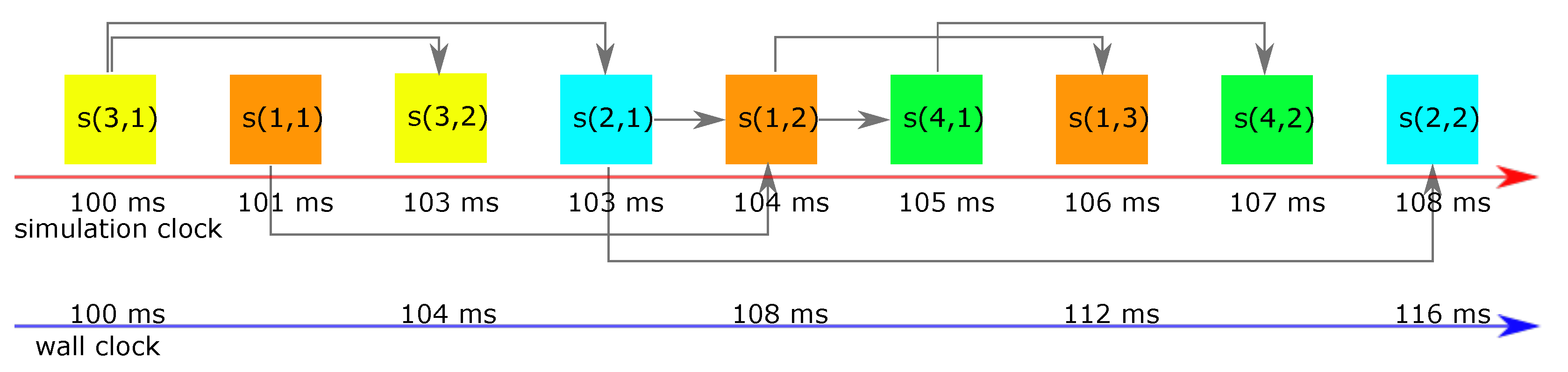
Figure 5 shows a possible execution path of the previously defined scenario in a conservatively synchronised environment with two workers. worker1 is calculating the states of $com{p}_3$ and $com{p}_4$. worker2 computes the states of $com{p}_1$ and $com{p}_2$. The colouring of components in Figure 5 matches the scheme in Figure 3; $com{p}_1$ is shown in orange, $com{p}_2$ is shown in blue, $com{p}_3$ is shown in yellow and $com{p}_4$ is shown in green. Grey arrows show dependencies between events executed on the same core. Additionally, dark green arrows show causal dependencies between states executed on different workers. Compared to single-core execution, the first set of states $s(3,1)$ and $s(3,2)$ can be executed in parallel to $s(1,1)$ and $s(2,1)$. To allow worker1 to process further, it has to wait until $s(1,2)$ was executed as this is a prerequisite for $s(4,1)$. The causal relation between $s(1,2)$ and $s(4,1)$ and therefore the knowledge about the required delaying of $s(4,1)$ is available throughout the lookahead information used in a conservative PDES.

Figure 6 shows the progression of $t_{dif}$ and $t_{ga{p}_{par}}$ during this conservatively simulated scenario. As explained for Equation (6), a negative $t_{gap}$, and consequently also a negative $t_{ga{p}_{par}}$, describes a system which is currently faster than real-time. Due to the parallel execution of events at the beginning of the scenario, the run is able to keep up with real-time until $t_w=104\mathrm{ms}$. After $t_w=104\mathrm{ms}$, the simulation stays one millisecond behind real-time. $t_{dif}$ shows the current synchronisation between the workers themselves. It can be seen that there is always a certain gap between the current simulation time of each worker, except for $t_w=104\mathrm{ms}$.

5.2. Optimistic PDEs

Figure 7 shows the introduced scenario executed using an optimistic synchronisation approach. The colour code is still remaining, similar to Figure 3 and Figure 5. Orange, blue, yellow and green boxes are events corresponding to their components. Grey and green arrows show intra- and inter-worker dependencies. Additionally, dashed dark green arrows show causal dependencies, which could not be satisfied. States with a red dashed border have to be rolled back because of a causal dependency violation. States without borders are not involved in a dependency violation.

Figure 8 reveals the behaviour of $t_{dif}$ and $t_{ga{p}_{par}}$ in this particular optimistic execution. Until $t_w=102\mathrm{ms}$, everything is equal to the conservatively synchronised scenario. However, at $t_w=104\mathrm{ms}$ worker1 does not wait until $s(1,2)$ was processed to continue with $s(4,1)$, which is initially the big advantage in optimistic simulations. Hence, also $s(4,2)$ will be processed at $t_w=106\mathrm{ms}$. This results in a real-time capable run until $t_w=108\mathrm{ms}$ compared to $t_w=104\mathrm{ms}$ for the conservative scenario. However, after processing of $s(4,1)$, the remote event scheduled by $s(1,2)$ arrives at worker1. Thus, states $s(4,1)$ and $s(4,2)$ have to be rolled back and have to be re-executed with the knowledge about the prerequisite of $s(1,2)$ for $s(4,1)$. This executed rollback causes $t_{ga{p}_{par}}\left(108\mathrm{ms}\right)$ to incline to $3\mathrm{ms}$. Also, $t_{dif}$ is rising steeply at this time point, caused by worker2 sticking to its simulation time and worker1 losing time caused by the rollback.

6. Significance and Applicability

Section 4 introduced a novel metric to evaluate the real-time behaviour of parallel executed DESs. It was shown, by means of example, that the metric can be applied for single-threaded simulations as well as for optimistic and conservative parallel simulations. However, the metric is not applicable for answering the question if real-time PDESs are possible without further knowledge of the system to simulate. Such a generalised statement is practically impossible as it highly depends on the used tools and the model’s domain. Thus, which preconditions have to be met by a simulation framework before the metric can be applied and which assertions the metric allows must be discussed.

6.1. Where Is the Metric Applicable?

The metric is designed to be used with any simulation model, which can be described using the Discrete Event System Specification [1] as long as the following rules apply:

• Model changes only apply at discrete time points
  According to Zeigler et al. [1], DES require state changes to happen only at specific points in time, at which an event is executed or applied. Between those time points, the model’s states are not allowed to alter. However, for the metric to be applicable, it is not required to have all events sorted into the FES before they occur. This is especially relevant when external hard- or software is connected to the simulation. Events generated asynchronously from such an external entity can be handled, as long as it is known at which time point these events should be executed in the simulation. If no time point is explicitly given for an external event, immediate processing of this event is implicitly requested. Consequently, $t_{ga{p}_{par}}$ must be calculated against the point in time where the request was received and the actual execution of the event.
• A real-time time base is available
  A prerequisite for the calculation of $t_{gap}$ is the availability of a real-time time base. This does not imply that any kind of real-time operating system must be involved in the model execution. However, the quality of the calculated real-time gap depends on the implementation of the used software clock. For example, C++ offers a steady clock (https://en.cppreference.com/w/cpp/chrono/steady_clock (accessed on 15 December 2020)), which guarantees the monotonic and uniform growth of its tick counter. However, the granularity is operating system specific.
• The simulation time can be mapped to the wall-clock time
  A mapping between wall-clock time and real time is required to calculate $t_{gap}$ as defined in Equation (5). Thus, the simulation tool must be capable of storing its exact start time $t_{wStart}$. Ideally, $t_{wStart}$ corresponds to the point in time where the simulation framework has finished the initial setup of the simulation model. This avoids erroneous results at the beginning of the simulation. If this is not possible, it is advisable to skip the first few seconds before performing further calculations as $t_{ga{p}_{sim}}$ or $t_{di{f}_{sim}}$.
• The current simulation time can be measured for all logical processes
  To calculate $t_{dif}$, it is mandatory that each logical process is aware of its current simulation time. This is not complicated for optimistic simulations, as they are usually not waiting for other logical processes to complete a certain task. In conservative simulations, however, a logical process may currently idle and wait for another logical process to finish. This behaviour is shown at $t_s=104\mathrm{ms}$ in Figure 5. Thus, the waiting logical process has to store the simulation time of the last executed event for calculation of $t_{dif}$, and therefore $t_{dif}$ tends to grow in such situations.

6.2. Which Statements Can Be Made Using the Metric?

As mentioned before, the metric alone is not capable of providing a generalised answer if a certain synchronisation scheme is well suited for real-time execution. Various factors, like the boundary conditions and the used operating system influence the significance of the metric. However, when all boundary conditions are known and taken into account the metric’s explanatory power remains unvaried.

6.2.1. Boundary Conditions

Many factors, further called boundary conditions, must be taken into account to make sure if a synchronisation scheme is well suited for real-time execution. Altering just one of these conditions can influence measurements significantly, so that a new validation process must be started. However, with exact knowledge of a certain use-case and its boundary conditions, the real-time capability of a simulation in this specific setup can be evaluated. Even more, if boundary conditions are only slightly changed, one may consult earlier findings to predict the real-time behaviour before starting a test run.

Table 2. Minimum set of boundary conditions to make the metric applicable.

Boundary	Description	Changes Frequently?	Example
System	What computing resources are available?	Does not change regularly.	Intel Xeon E7-8867 v4 @2.40GHz, 4 × 18 cores, 3TB RAM, 450GB SAS SSD RAID1
Real-time type	Is the threshold hard, soft or firm real-time? [11]	Does not change regularly. Highly dependent on the domain.	Hard real time is required. Exceeding a threshold is never allowed.
$t_{ga{p}_{sim}}$ threshold	How high is $t_{ga{p}_{sim}}$ allowed to be?	Does not change regularly. Highly dependent on the domain.	Set to 300 ms for real-time human interaction [20].
$t_{di{f}_{sim}}$ threshold	How high is $t_{di{f}_{sim}}$ allowed to be?	Does not change regularly. Highly dependent on the domain.	Set to 100 ms to meet $t_{ga{p}_{sim}}$ threshold.
Framework	Which simulation framework is used to simulate the model?	Decided once.	OMNeT++ 5.6.2 using command-line environment (Cmdenv)
Configuration	How is the simulation framework configured?	Can change during the life cycle.	Framework and model is configured to use Null Message for synchronisation.
Model	Exact definition of the simulated scenario	Changes frequently	VANET scenario with 50 active vehicles is employed. Nakagami fading is used as channel model.

shows a minimal set of boundary conditions that apply to almost every use case. However, this table is by no means complete, and several other conditions might apply in other use cases. Its first two columns describe the type of boundary condition. Column three gives how often these conditions usually change. For example, the used system and framework, as well as the real-time requirements, do not frequently change during test execution. However, model complexity will change frequently. The last column gives an example of each identified boundary condition.

Frequently changing all of the boundary conditions would lead to unpredictable real-time behaviour. However, if a model designer decides against altering the boundary conditions except the model description, which includes the exact definition of the simulated scenario, it can be assumed that proper predictions can be achieved. For example, if several measurements with a certain scenario complexity were carried out and these measurements indicated real-time capabilities, it can be assumed that other runs with similar or less complex scenarios will be real-time capable.

6.2.2. Influences of the Operating System

The operating system used to execute the simulation has a major impact on the metric’s significance. The results provided by the metric can only be as accurate as the time stamping provided by the underlying operating system. Non-real-time operating systems like off-the-shelf Linux distributions offer a monotonic clock with an accuracy of at least one microsecond. This implies that the metric can expose the real-time capabilities of a simulation within these accuracy thresholds [37]. Real-time operating systems can provide finer-grained timing information. However, executing software under hard real-time restrictions implies that certain deadlines are never violated in the first place [11,12]: A real-time capable operating system guarantees that tasks are executed within a given time span. This implies that the proposed metric is not required to measure the real-time gap on a real-time operating system, as the system itself provides suitable mechanisms to never violate any given deadline. Hence, the metric’s application area will be soft and firm real-time DESs, independent if they are executed sequential or in parallel.

6.3. Evaluation of a Sequentially Executed Real-World Simulation

Obermaier et al. [7] present a closed-loop simulation for VANET devices. It is based on the Artery framework for OMNeT++ [38]. A mandatory requirement for HIL simulation is the real-time capability of a test run. As shown by Neumeier et al. [39], speeding up a wireless simulation framework for OMNeT++ is a complicated task. Even more, introducing parallelism in an already existing model is hard to accomplish. Thus, Obermaier and Facchi [40] investigated the real-time capabilities of Artery as a single-core DES.

Applying the novel metric to the simulation run explained in [40] prompts the following restrictions: As sequentially executed simulations do not employ several workers, $t_{di{f}_{sim}}$ is not applicable. Even more, $t_{ga{p}_{par}}$ equals $t_{gap}$; thus, Equation (6) is employed for the calculation of $t_{ga{p}_{sim}}$. Two different scenarios presented in [40] are utilised to evaluate the real-time capabilities of the simulation runs. Figure 9 and Figure 10 show the real-time behaviour during the simulation. These scenarios consist of three and five active vehicles communicating with each other via IEEE 802.11p using a shared wireless channel. The red line shows $t_{gap}\left(t_s\right)$, which is rising and declining during the ongoing simulation. The boundary conditions defined in

Table 3. Boundary conditions for the real-world example taken from [7].

Boundary Condition	Value
System	Cluster: Intel Xeon E7-8867 v4 @2.40GHz, 4 × 18 cores, 3TB RAM, 450 GB SAS SSD RAID1 and Laptop: Core i5-6300U @2.40GHz, 1 × 4 cores, 16 GB RAM, 256 GB SSD
Operating system	Cluster: openSUSE Leap 15.2 without real-time extensions and Laptop: Ubuntu 18.04 without real-time extensions
Real-time type	Soft real time
$t_{ga{p}_{sim}}$ threshold	0.02 s
$t_{di{f}_{sim}}$ threshold	Not applicable as no parallelism was involved.
Framework	OMNeT++
Configuration	The Artery model for OMNeT++ was used with standard configuration.
Model	A three-vehicle scenario and a five vehicle scenario was employed.

are used to carry out the measurements. Based on these conditions,

Table 4. Evaluation of the real-time capabilities of the simulation runs presented in [40]. Due to the single-core execution of the scenario, $t_{di{f}_{sim}}$ is never available. Result evaluations are derived from findings in [7].

Run Description	${\mathit{t}}_{{\mathit{gap}}_{\mathit{sim}}}$	${\mathit{t}}_{{\mathit{dif}}_{\mathit{sim}}}$	Result
3 vehicles (laptop)	$0.04$ s	$N/A$	Exceeds real-time threshold of 0.02 s
3 vehicles (cluster)	$0.013$ s	$N/A$	Does not exceed the real-time threshold of 0.02 s
5 vehicles (laptop)	$0.07$ s	$N/A$	Exceeds real-time threshold of 0.02 s
5 vehicles (cluster)	$0.04$	$N/A$	Exceeds real-time threshold of 0.02 s

summarises the outcomes after the metric has been applied.

7. Conclusions and Further Work

This paper focuses on providing a connection between PDES and DES executed in soft or firm real-time. An intensive literature review revealed that PDESs aim for enhancing the execution speed of a certain simulation model typically, but not for real-time simulation. Established definitions from Zeigler et al. [1] have been revisited to formally define deterministic DES and create a common understanding. Fujimoto [2] provided a formula to calculate the expected simulation time at a certain wall-clock time for simulations executed in real time. Employing theses foundations, an easy to calculate yet expressive metric for the real-time capabilities of a PDES synchronisation scheme is proposed. The metric is based on two elementary values: $t_{ga{p}_{par}}$ and $t_{dif}$. While $t_{ga{p}_{par}}$ is the current real-time loss in a parallel simulation, $t_{dif}$ informs about the internal synchronisation of the different execution contexts. Depending on the outcomes of $t_{ga{p}_{par}}$ and $t_{dif}$ calculations, the real-time capability of a simulation run can be ranked. The metric is applicable to any DES that meets the following requirements:

• Model changes are bound to discrete time points.
• A real-time time base must be available on the system.
• The simulation time can be mapped to a wall-clock time using Equation (5).
• Each logical process is able to measure its own simulation time.

Whenever a DES fulfils these requirements and in-depth knowledge about the to-be-simulated system its boundary conditions is available, the real-time capabilities of a simulation run can be measured and finally predicted. Boundary conditions can be but are not limited to hardware resources, type of required real-time, real-time threshold, the used simulation framework and its configuration, as well as the model to be executed. It is shown that the metric’s significance is influenced by the used operating system and the employed clock for measuring time. The metric is applicable in soft and firm real-time situations, where the system guarantees no timing. On systems fulfilling hard real-time requirements, the metrics add no further information beyond the system’s guarantee to execute tasks within a defined deadline.

This paper also shows how the metric can be applied to conservative as well as optimistic synchronisation schemes of PDESs using a synthetic example scenario. However, a synthetic example does only allow a very vague prediction of the real-time capabilities of realistic simulation runs. Thus, further investigations and measurements must be carried out to allow a reliable interpretation. This includes the determination of boundary conditions for various use cases and measuring their influences on real-time behaviour.

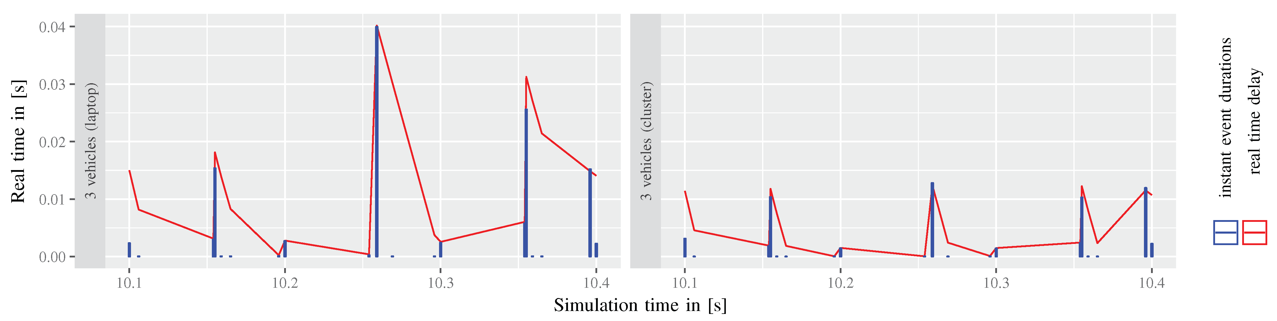
The real-time capability investigations of the OMNeT++ simulation framework by Obermaier and Facchi [40] were re-evaluated to clarify the usage of the introduced metric using a real world example. Boundary conditions for this specific use-case are derived and presented. Even though the simulation is executed on a single core, and therefore $t_{dif}=N/A$, it was shown how the metric enables comparability of simulation runs with respect to their real-time capabilities and how these results react on altering of boundary conditions.

It can be concluded that the introduced metric benchmarks the real-time capabilities of a simulation framework or a simulation run. However, definite assertions depend on the existence of appropriate boundary conditions. As these highly depend on the given use case, they have to be elaborated for each domain of real-time simulation individually. In future work, the proposed metric can be used to easily rank new simulation frameworks with already existing frameworks when proper boundary conditions are defined. This allows a further investigation and finally an estimation of which synchronisation scheme might be most appropriate for PDESs executed in a real-time fashion.