Using Actors and Use Cases for Software Size Estimation

Abstract

Software size estimation represents a complex task, which is based on data analysis or on an algorithmic estimation approach. Software size estimation is a nontrivial task, which is important for software project planning and management. In this paper, a new method called Actors and Use Cases Size Estimation is proposed. The new method is based on the number of actors and use cases only. The method is based on stepwise regression and led to a very significant reduction in errors when estimating the size of software systems compared to Use Case Points-based methods. The proposed method is independent of Use Case Points, which allows the elimination of the effect of the inaccurate determination of Use Case Points components, because such components are not used in the proposed method.

1. Introduction

The determination of the software system size is one of the key activities that must be performed when planning the time or resources necessary for its development. An estimate of the software system size is understood to mean the determination of its resulting size, i.e., the number of functions that the software system should provide. To estimate the size, it is possible to use various methods. These methods differ according to the underlying principle, the required data, and the quantity for which the estimate is performed. The Use Case Points (UCP) method is often used for estimation purposes [1] in the early development phase.

The development of software system size estimation includes methods based on the number of lines of source code, which were described in various forms [2,3,4] and subsequently modified [5,6,7,8]. Other methods include those based on the analysis of functional points [9] and those based on finding similarities between a new software system that is to be designed and systems that were completed earlier [10].

The objective of utilizing such estimation methods is to find the relationship between the available description of a project in the early phase of the development of a software system and its final size. One of the main criteria for assessing the quality of the estimation is the size of the error that arises during such an estimation. An error is understood to mean the difference between the actual size (after the completion of the development of a project) and the estimated size value.

The estimate should be performed as soon as possible, i.e., in the early phase of a project. Methods that are based on use case models suit this requirement. Use case models are represented by a graphic and verbal description of a software project’s planned functionality.

The Use Case Points method, the basis of which utilizes actors and use cases, was designed by Gustav Karner in 1993 [1]. Among the main disadvantages of this method, which is still applied to this day, are the dependency on the method for calculating sub-components and the potential introduction of errors. Potential errors can arise from the personal interpretation of the method and the manner in which the descriptive parameters are stipulated. Other shortcomings stem from the properties of the use case model and the method by which it is processed. In ref. [11], the authors discuss the effects of extension associations on the accuracy of the calculation, whereby their proposed procedure enables more accurate calculations. The authors also try to make the estimate more accurate [12,13].

A resolution of the shortcomings of the Use Case Points method is often proposed on the basis of an analogy between projects [10,14]. In cases where the task is not to estimate the size of a proposed software system, but the realization time, the calculation must also include the effort value [15], i.e., the ratio between one point of size and the number of person-hours required to implement it.

The main group consists of new approaches to the calculation of sub-components [16]; these are mainly the Extended UCP [15] and Modified UCP [17] methods. In addition, there are modifications that relate to the processing of scenarios [18], where other possibilities for ascertaining the number of steps are sought by using transactions or paths in a scenario. The common approach is based on the total number of steps in a scenario, which is a simple and straightforward solution. In the case of transactions, related steps, which form a complete activity, are identified within a scenario. For example, a scenario may contain eight steps, which can be divided into two related transactions. One of the approaches [18] for determining the number of transactions is based on the number of transactions being equal to the number of stimuli. The stimulus is understood to mean the number of external interactions—inputs in a given use case. Another work that discusses the issue of transaction identification is ref. [19]. In this work, the main objective is to increase the reliability and repeatability of the calculation method. Some authors in ref. [20] also analyze events in scenarios so that they can therefore identify transactions. Overall, the effect of transactions can be described as questionable because it does not guarantee the possibility of repeatability, even in the event of the utilization of an identical use case. Room is still given here for individual interpretation by the estimator.

The internal structure of the scenarios [16] is regarded as a key factor. The proposed approach should lead to a better evaluation of the actors and use cases alike. The effect of scenarios, and the method by which they are accounted for, is frequently examined. However, it remains questionable whether the benefit is sufficient to justify the higher complexity of the calculation.

In the literature, alternative approaches for modifying UCP methods can also be found. For example, the authors [15] utilize Bayesian networks and fuzzy sets to create a probability estimation model.

If the actors and use cases are precisely defined, then an accurate estimate can be achieved using technical and environmental factors [17], and therefore, points that are already estimated can be regarded as a suitable system size value [17].

Another UCP modification is the Adapted UCP [21] method. This modification was created for the estimation of large projects. This approach is based on the assumption that, in the first iteration, all actors are regarded as averagely complex and all use cases as complex. In contrast, Ochodek [22] recommends that actors be omitted completely as model attributes. However, this is in conflict with the performed analysis [23]. According to ref. [22], it is also appropriate to perform a decomposition of scenarios, leading to their division into scenarios with a smaller number of steps.

Methods based on analogy, which can be understood as another problem resolution option during estimation, are dealt with by the authors in ref. [24].

The significance of the elements of the UCP method is partially discussed in the work [22,23,24,25,26,27,28,29] and also in refs. [12,13], where the utilization of a linear regression model is proposed. However, these works do not prioritize the significance of the elements; instead, they mainly communicate the basic applications of regression models.

Regression models (RegA) and a neural network model, multiple perceptron (MLP), are also studied by Nassif in the work [27], where a regression model with a logarithmic transformation is presented. In their subsequent work, Nassif and Capretz [27] also deal with multiple regression but only to determine productivity and not to estimate the size of a proposed software system [30]. In ref. [31], Nassif and Capretz discuss the artificial neural network (ANN) model and log-transformed linear regression model (RegB).

In the work [23], the process of using a regression model constructed with the help of the stepwise regression method (StepR) is presented. In ref. [29], Silhavy et al. compare the following methods, which improves the UCP approach: k-means clustering (KM), spectral clustering (SC), and moving windows (MW) [30]. In ref. [31], Azzeh et al. discuss setting a productivity factor using a new ensemble construction method and compare this approach to MLR or StepR. The described approach can be used for size estimation, but it works with person-hours (effort), too. In ref. [31,32] Nassif et al. discuss applications of fuzzy sets for effort estimation.

Section 2 defines the problem to be resolved and sets out the basic research questions. Section 3 describes the theoretical standpoints. Section 4 describes the performed experiments and the results thereof. Section 5 is a discussion of the results, from which conclusions are drawn and presented in Section 6, including directions for further research.

2. Problem Statement

As the aforementioned literature research reveals, until now, only methods that led to the further specification of the UCP method were examined. However, the objective of this article is to put forward a new, simplified method based purely on the number of actors and use cases. As the aforementioned literature research also shows, the methods that led to the specification of UCP are beneficial for achieving higher estimate accuracy. However, they are still based on the need to estimate the elements of the UCP method, whereby the quality of the input data will affect the resulting estimate accuracy [23,29,33].

The proposed method, called Actors and Use Cases Size Estimation (AUCSE), works with the numbers of actors and scenarios only. This conceptual idea was firstly introduced by the authors of this paper in ref. [34].

Actors and Use Cases are divided into three groups according to complexity. In this aspect, this proposal is based on the UCP method.

The resulting size estimate will be stated in UCP, but the common procedure for calculating UCP will not be used for the estimation. The proposed method is not based on UCP components [34].

If it is proven to be usable, this approach will lead to the potential creation of an effective and sufficiently accurate estimation method.

The point of this experiment is to verify whether the entire estimation process can be simplified and made without Use Case Points methodology. On the basis of the aforementioned, the following research questions were formulated:

• RQ1: What is the significance and benefit of the number of actors and use cases for size estimation?
• RQ2: Is the proposed new method AUCSE more accurate than Use Case Points or other selected Use Case Points methods?

Therefore, the suitability of actors and use cases as independent variables, which can be used for a simplified estimate process in comparison to the UCP method, will be examined.

3. Methods

Use case modeling is one of the basic functional analyses for software systems [35,36,37,38]. It involves the graphic and verbal capturing of the target functionality of the software system to be developed. This approach is defined as part of the object-modeling language (Unified Modeling Language, UML). In use cases, the functionality (algorithm) is captured either in the form of a structured scenario or in the form of free text.

Use case modeling enables the further elaboration and improved analysis of a software project´s functional requirements, as collected during a project’s initial phase. Use case modeling can be understood as an alternative method for capturing requirements [36,37], which are processed, and if applicable, modeled within the scope of engineering requirements [38]. The basic activities of use case modeling include the following [39]:

• Determination of the software system’s boundaries;
• Derivation of the software system’s actors;
• Derivation of main use cases;
• Finding alternative use cases.

The aforementioned activities are performed repeatedly until development progresses to a phase in which the required behavior of the software system no longer changes.

Use case modeling is based on all available information sources. It is the most significant analysis of the activity of an organization in which a software project is to be deployed [38].

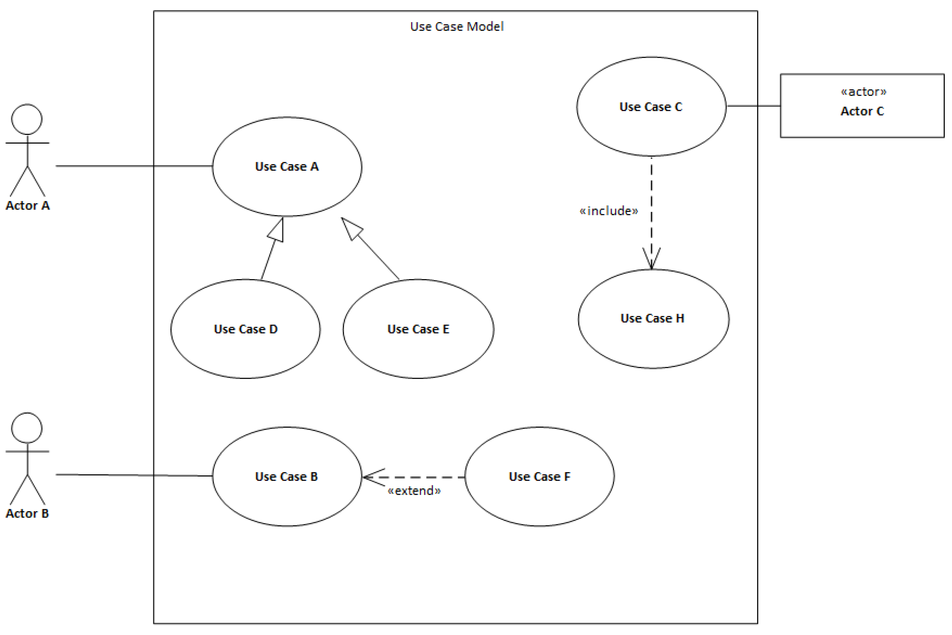
The determination of a system’s boundaries is key to determining the extent of the services and functions provided by a proposed system. The boundaries are defined graphically in a model, but their significance is given through content. The boundaries are defined by the system’s surroundings, actors, and use cases.

Therefore, the point is to define which functions will be developed and which functions already belong in the surrounding systems, i.e., systems collaborating/communicating with the system to be developed.

The example in Figure 1 represents a use case model that depicts a system’s boundaries, actors, use cases, and possible mutual relationships between use cases.

An actor is the specification of a role, in the sense of an external entity, which communicates with the system and thus utilizes use cases within the system’s boundaries. An actor can be understood to be a role, whereby the role can represent many physical objects of the same type. Therefore, an actor does not represent only physical users but also other software systems in the vicinity. In the case of actors, one important rule applies, namely that the system itself is not an actor. However, this does not mean that there are no internal representations of actors in the form of objects or classes. If an activity that is set off by a timed event needs to be modeled in the system, then time is modeled as an actor. Therefore, an actor can be understood to mean a user working with the application or a collaborating system’s application interface. Time is modeled as an actor where an activity starts at a certain time or interval. An example of its use is the generation of a notification in a calendar, or the sending of a reminder.

A use case represents a certain function or activity that is available for a chosen actor. It is the specification of the order of activities (scenario) that describe the interactions between the actors and the modeled system. Use cases contain main scenarios, which capture the correct progress of an interaction. It is also possible to capture alternative scenarios, which serve to capture behavior in the event of an exception or erroneous situation.

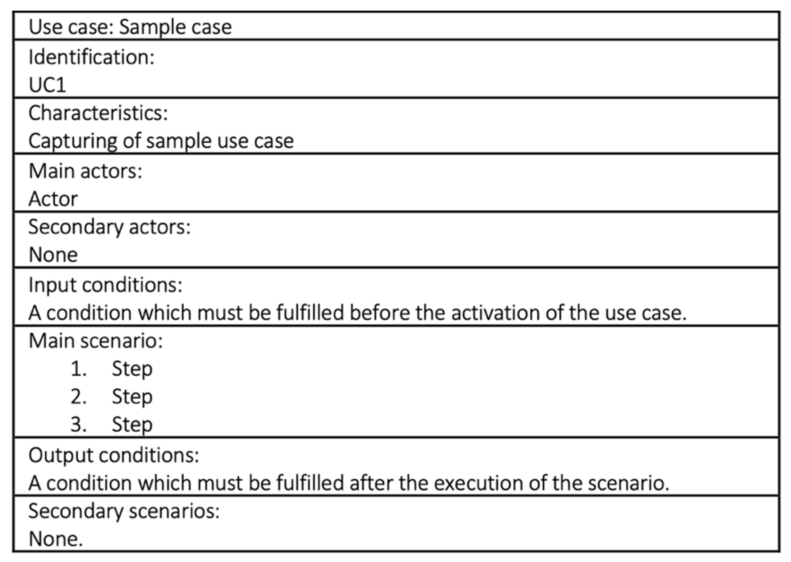
Scenarios represent a core part of the use case model for the determination of a proposed software system’s behavior. The general structure of a scenario in the use case model (Figure 2) contains information regarding the name of the use case, its identification, brief characteristics, a list of actors, and the scenario itself.

A mandatory field structure is not prescribed in UML language. It is assumed that use cases describe a system’s activity; therefore, the individual names should be based on or contain a verb phrase. A name must be chosen that is brief, apt, and comprehensible. Steps in the scenario represent activities in chronological order, which are either performed by an actor or the proposed system. It is for this reason that we talk about capturing the interaction between the actor and the proposed system. The individual steps are entered in the form of brief and apt sentences. The objective is to limit, as much as possible, the possibility of varying interpretations by individual model users.

3.1. Stepwise Regresssion

Stepwise regression methods are based on multiple linear regression, whereby the gradual elimination of independent variables, which are not beneficial for the quality of the model, takes place on the basis of chosen criteria and the level of significance.

Stepwise regression combines the methods for the descending and ascending selection of independent variables. For decision-making, the chosen threshold value is used. Therefore, the independent variables whose threshold is within the required interval remain unaffected.

Descending selection works by including all of the available independent variables in the default model, and then, in every step, eliminating the independent variable that contributes the least to the explanation of the dependent variable. All of the variables with a threshold value (in terms of absolute value) greater than the chosen boundary are eliminated.

Ascending selection works by not including any available independent variables in the default model; instead, only a constant component is utilized. In every subsequent step, the independent variable whose threshold value is the highest is added to the model. The ascending selection ends if the threshold values of all of the included independent variables are lower, in terms of absolute value, than the chosen boundary value. The stepwise regression procedure enables the testing, on chosen training dates, of models with various default configurations, whereby the objective is to find a suitable set of independent variables [29,40,41].

The process can be summarized as follows:

• Selection of the default model required if the descending principle is used, or selection of an empty model for the ascending approach.
• Setting of the resulting model—only linear components, quadratic components, etc.
• Selection of the threshold value for the addition and removal of independent variables.
• Addition and removal of suitable independent variables and repeated testing.
• The algorithm ends when the model contains only suitable independent variables.

3.2. Actors and Use Cases Size Estimation Method Design

In the following analysis of the significance of the number of actors and use cases, the objective is to show how Actors and Use Cases Size Estimation (AUCSE) was designed. The principle of the method, which favors it in comparison with the UCP method and also with UCP method’s modifications, is that it only works with the numbers of actors and scenarios. These numbers are divided into three groups according to complexity. This leads to the derivation of independent variables Actor 1–3 and Case 1–3. According to the analysis, technical factors (variables T1–T13) and environmental factors (variables E1–E8) have a small practical impact.

Therefore, the principle of the AUCSE method can be summarized as follows:

• Identification of the actors and use cases from the use case model.
• Division into groups according to complexity (simple, medium, and complex). A similar approach, known from the UCP method [1], is used for the actors. For use cases, transactions are identified from the number of steps in the scenario [23].
• Subsequent division of the data in the dataset on the basis of the hold-out approach and the design of an estimation model in the training part on the basis of the stepwise regression method.
• Estimation of the new project based on the use of the identified numbers of actors and use cases in the model as input variables.

4. Experimental Design

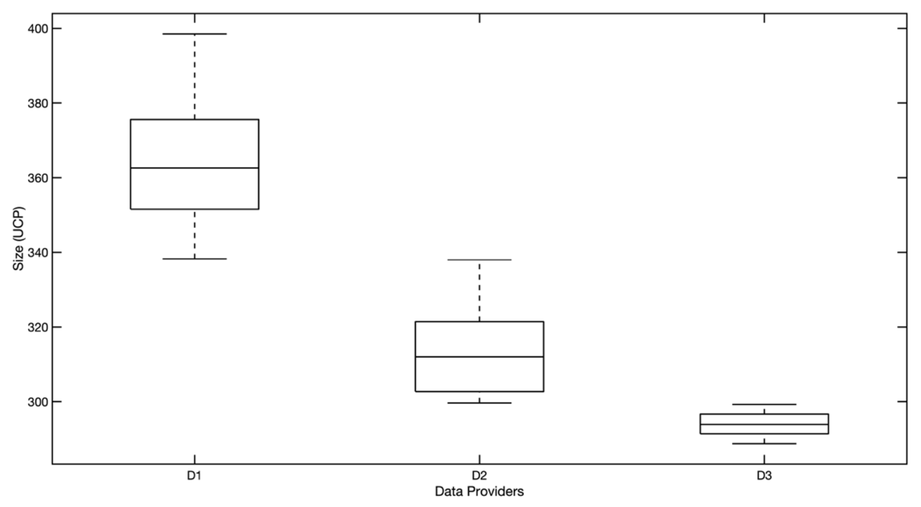
The dataset (DS) used contained a total of 70 observations (every observation representing a description of one realized software system) from three data providers [23]. DS is available as Supplementary Material. From the provided information, it follows (Figure 3) that data provider/supplier D1 realized the largest projects, and D3 had the smallest projects.

The DS contains a total of 20 attributes (

Table 1. Descriptive characteristics—dataset (DS).

Attribute	Median	Average	Standard Deviation	Size	Min	Max
UAW	8	10.49	5.02	13	6	19
UUCW	355	386.21	88.91	360	250	610
TCF	0.94	0.92	0.11	0.41	0.71	1.12
ECF	0.89	0.86	0.12	0.58	0.51	1.09
UCP (Real)	320.3	327.94	33.21	109.75	288.75	398.5
T1	0	0.41	1.15	5	0	5
T2	2	2	0	0	2	2
T3	0	1.36	2.02	5	0	5
T4	1	2.3	2.37	5	0	5
T5	5	2.93	2.37	5	0	5
T6	5	3.14	2.43	5	0	5
T7	5	3.71	2.07	5	0	5
T8	1	1	0	0	1	1
T9	5	4	1.96	5	0	5
T10	5	4.47	1.43	5	0	5
T11	5	4.9	0.39	2	3	5
T12	1	1	0	0	1	1
T13	1	1	0	0	1	1
E1	0	0	0	0	0	0
E2	0	0.04	0.27	2	0	2
E3	0	0.19	0.73	5	0	5
E4	0.5	1.21	1.37	4	0	4
E5	3	2.64	1.88	5	0	5
E6	4	4.16	1.02	4	1	5
E7	1	1.57	1.56	5	0	5
E8	4	3.84	1.26	5	0	5
Actor 1	0.5	0.71	0.9	4	0	4
Actor 2	1	0.94	0.88	3	0	3
Actor 3	2	2.63	1.51	6	0	6
Case 1	2	2.7	2.9	20	0	20
Case 2	15	15.84	5.37	27	3	30
Case 3	15	14.29	4.45	22	5	27
Problem Domain	Categorical variable			-	-	-
Language	Categorical variable			-	-	-
Methodology	Categorical variable			-	-	-
SW Type	Categorical variable			-	-	-
Data Provider	Categorical variable			-	-	-

). The first group consists of the attributes necessary for the UCP method Unadjusted Actor Weight (UAW), Unadjusted Use Case Weight (UUCW), Technical Complexity Factors (TCF), Environmental Complexity Factors (ECF) and UCP (Real). This group also includes the attributes T1–T13, which represent weights for technical factors, and the attributes E1–E8, which represent weights for environmental factors.

The second group is represented by attributes that quantify the number of actors (Actor 1, Actor 2, Actor 3) and the number of use cases (Case 1, Case 2, Case 3).

The last group of attributes is formed by the categorical attributes Problem Domain, Language, Methodology, SW Type, and Data Provider, which enable the project to be characterized in more detail.

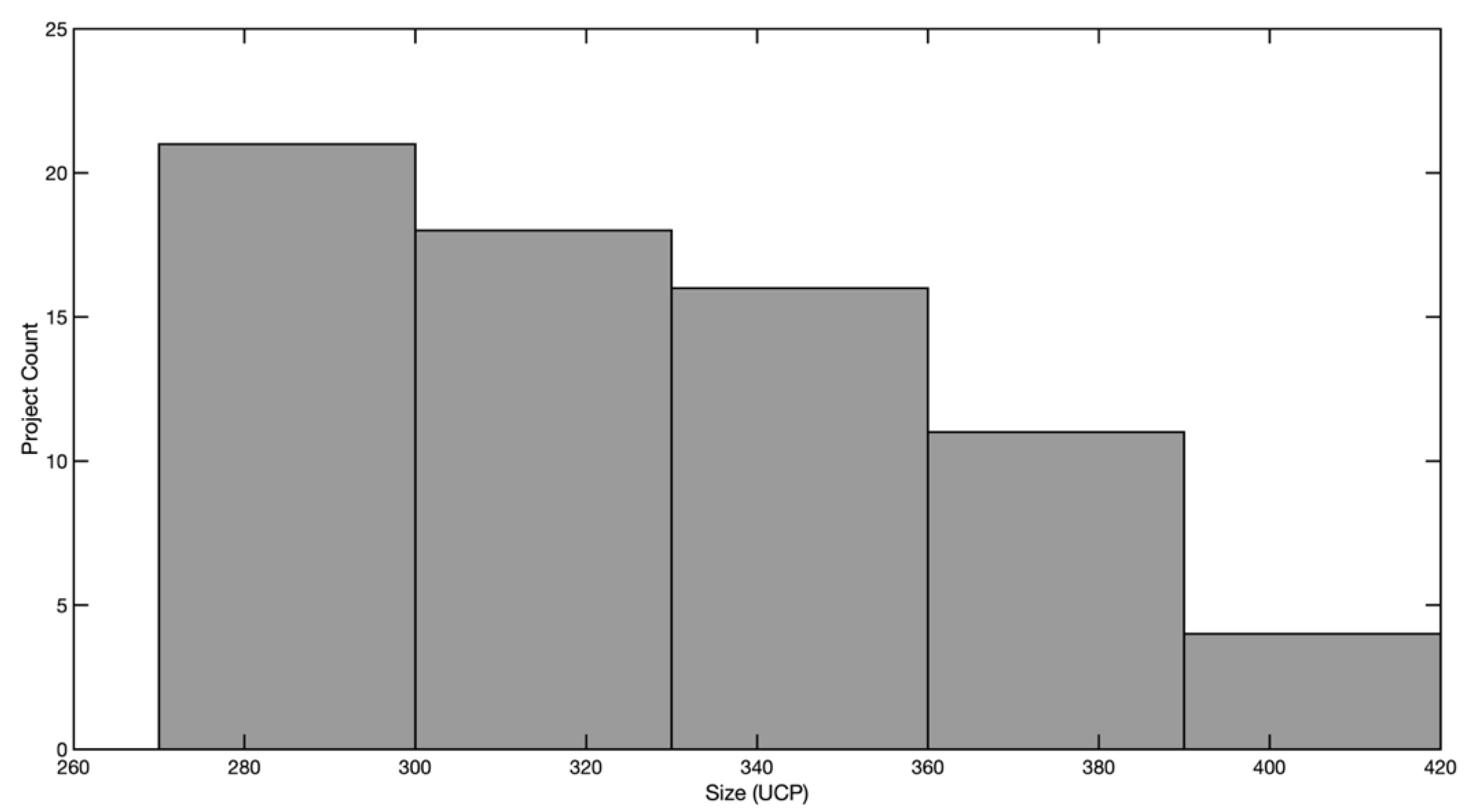
The overall project frequency distribution, while taking into consideration the actual size of the software systems in UCP, is captured in the following histogram (Figure 4).

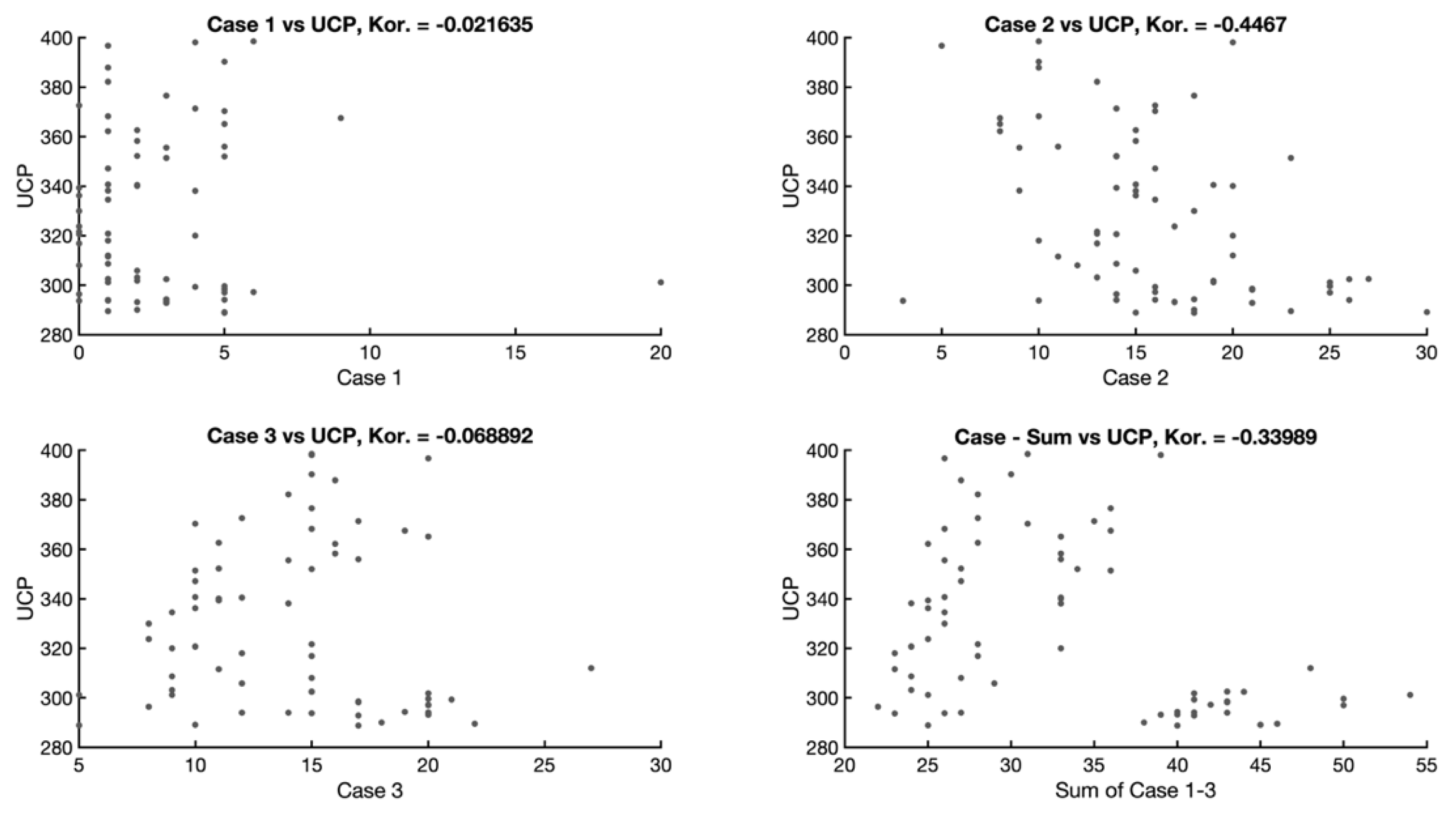
An interesting perspective on dependency is provided by the possible correlation between the total number of use cases and the individual complexity of the use cases (Figure 5). More significant correlations can be observed between the real size and use cases with average complexity and between the real size and the total number of use cases. Indicative of this fact is that averagely complex use cases are the most represented and the number of use cases in the other groups (according to complexity) is only weakly correlated.

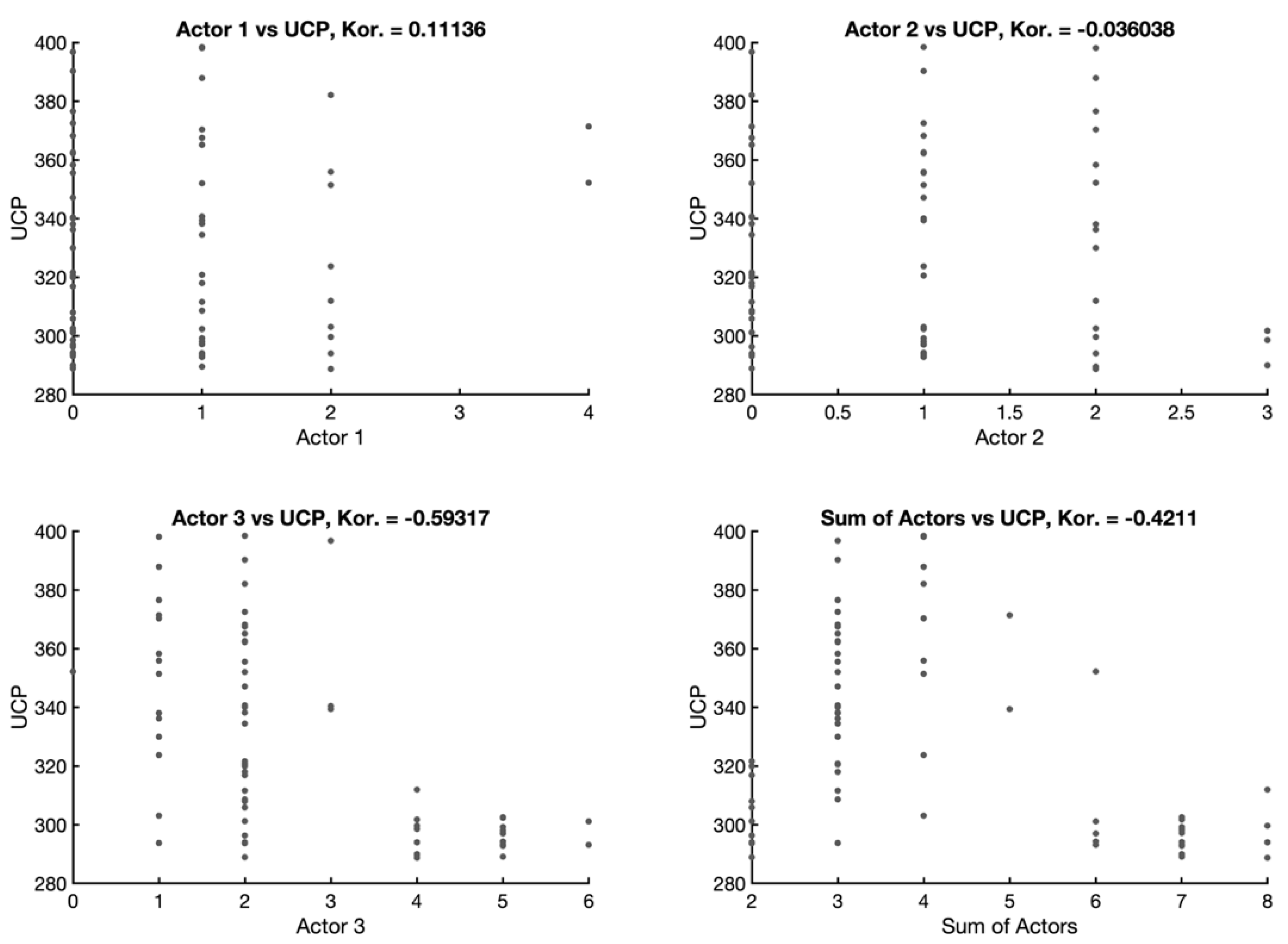
A similar situation can be seen when looking at the actors (Figure 6), whereby the strongest dependency can be seen between the attribute Actor 3 and the attribute UCP (−0.59). Dataset DS contains, to a large extent, regular company software systems in which actors are included in groups of complex actors that, to a greater degree, occur naturally.

The relationship between the weights T1–T13 and E1–E8 is not captured because it has no practical significance for further analysis.

In the studied Dataset attributes, a relationship with the real size of the software systems (UCP) was demonstrated. In the case of some attributes of the UCP method, the relationship is weak (TCF, ECF). Some groups of actors and use cases (Actor 1, Actor 2, Case 1 and Case 3) also have a weak relationship. However, this can be described as a natural and expected phenomenon. These groups are less represented during the design of software systems within the scope of all three (D1–D3) data providers.

For the purposes of this contribution, the dataset was divided into a training and testing part using the hold-out approach. Both datasets were divided into training and testing parts in a ratio of 2:1. This approach was chosen due to its frequent use in previously published works focused on the estimation of the size and development effort of software systems [29,34,42].

4.1. Actors as Independent Variables

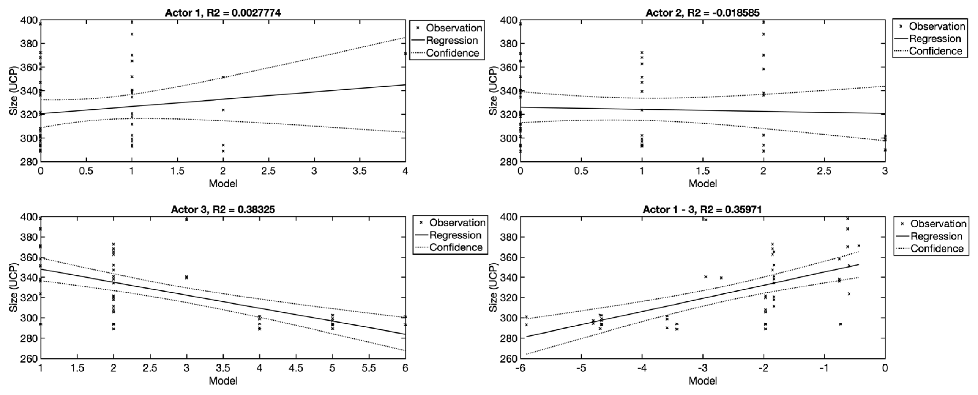
The characteristics of the actors (Actor 1–3) are set forth in (Figure 7). The use of actors will be examined on the basis of linear regression models. For this purpose, four regression models were created, of which three show the use of individual groups of actors separately (Actor 1–3), and the fourth shows all the groups of actors used as independent variables. For comparative purposes, a fifth model was also created that worked with the total number of actors.

From Figure 7, it is evident that the Actor 1 and Actor 2 variables are not suitable for the estimation. The reason for this is that they represent simple and averagely complex actors who are represented to a small extent in the training part of the dataset (DS) (usually 0 or 1 per observation). The number of actors with high complexity (Actor 3) is more variable in individual observations, which is why the model is able to explain approximately 40% of dependent variables.

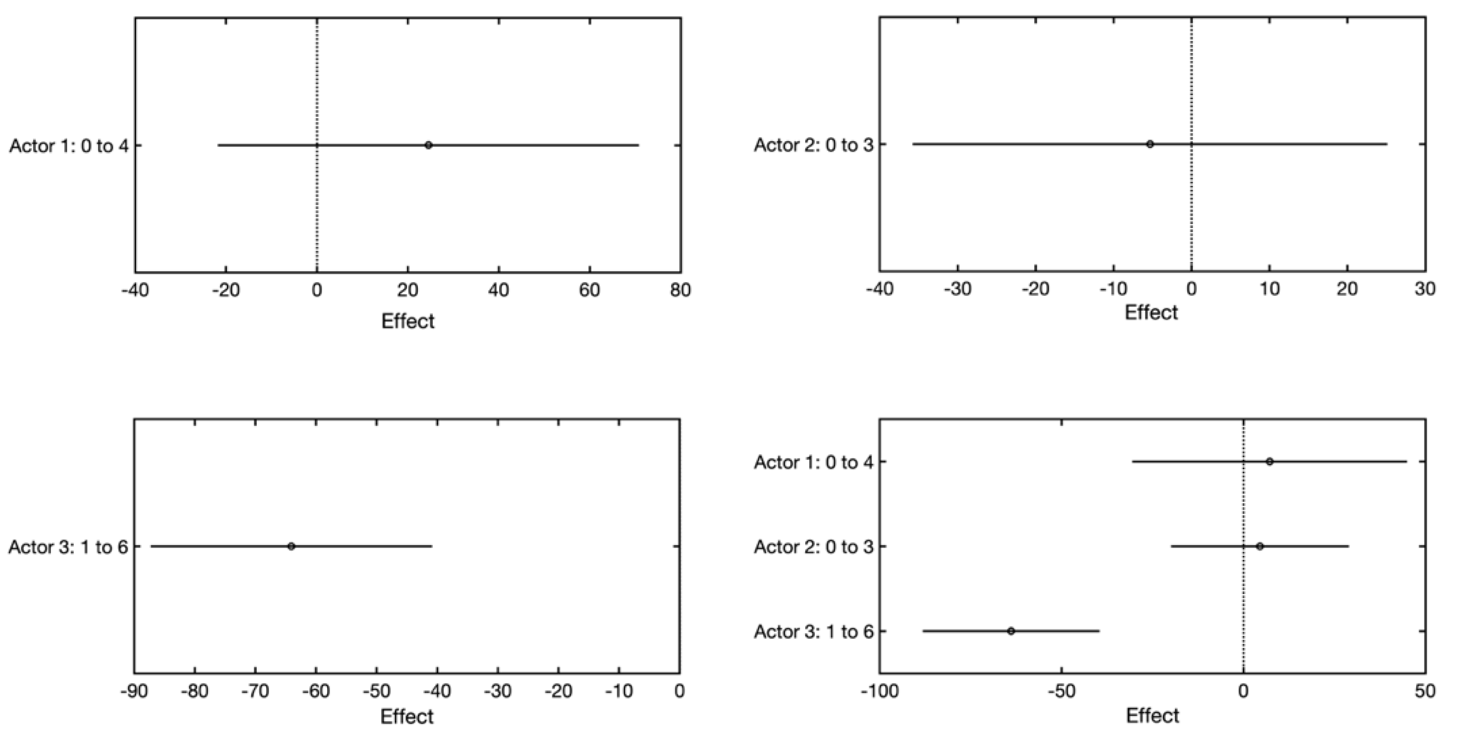
A closer look at the effect of the models (Figure 8) confirms the aforementioned. This graph shows how the estimation of the value of the dependent variable changes with the aforementioned change of the independent variable. From the figure, it follows that only Actor 3 has a significant effect on the change of the dependent variable. In the other cases (Actor 1–3), this effect is not statistically significant.

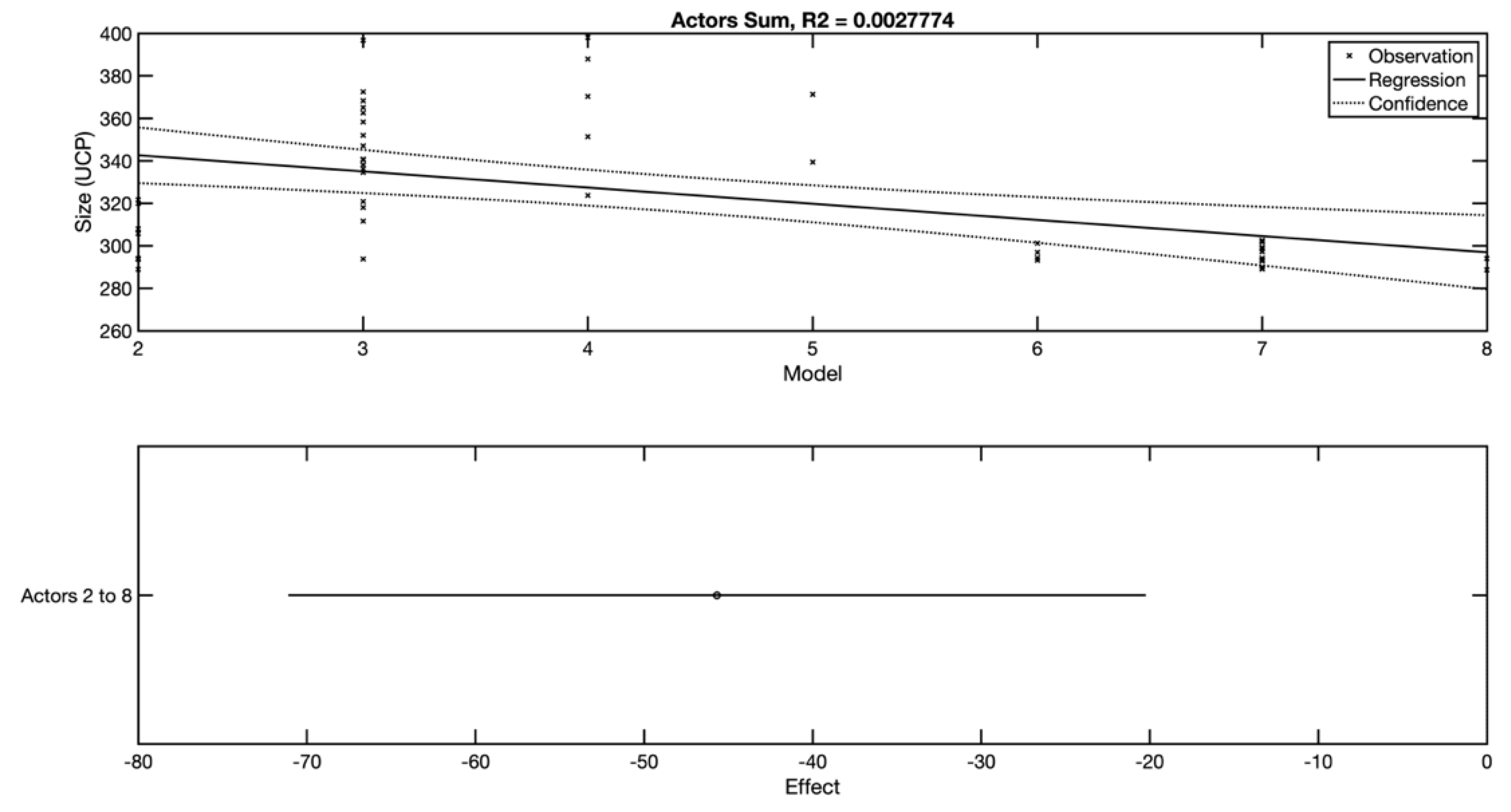
By simplifying the view and adding together all the actors—regardless of their complexity—the model (Figure 9) is obtained, on the basis of which it is possible to state that the total number of actors is not a suitable independent variable for the linear regression model. The ability to estimate the real size is not sufficient. The bottom part of the figure illustrates the dependency of the size of the software system on the change of the total number of actors (from 2 to 8).

4.2. Use Case as Independent Variables

The relationship between the number of use cases and the size of the software system measured in points (UCP) is examined here.

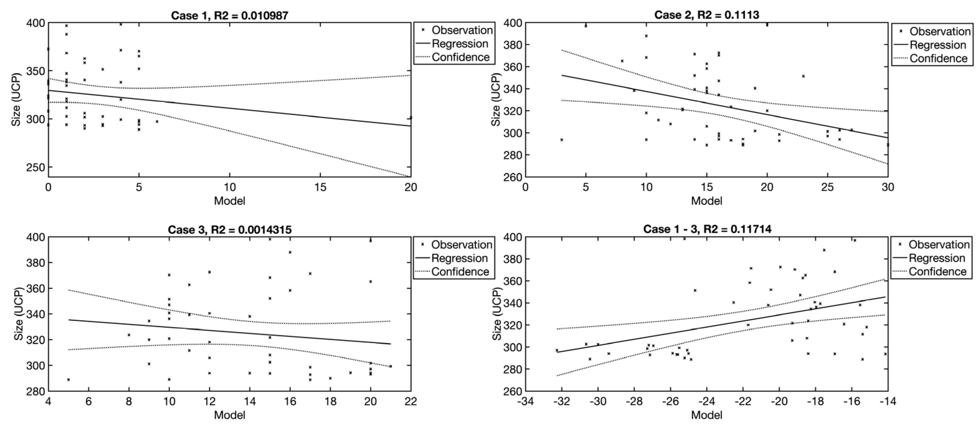
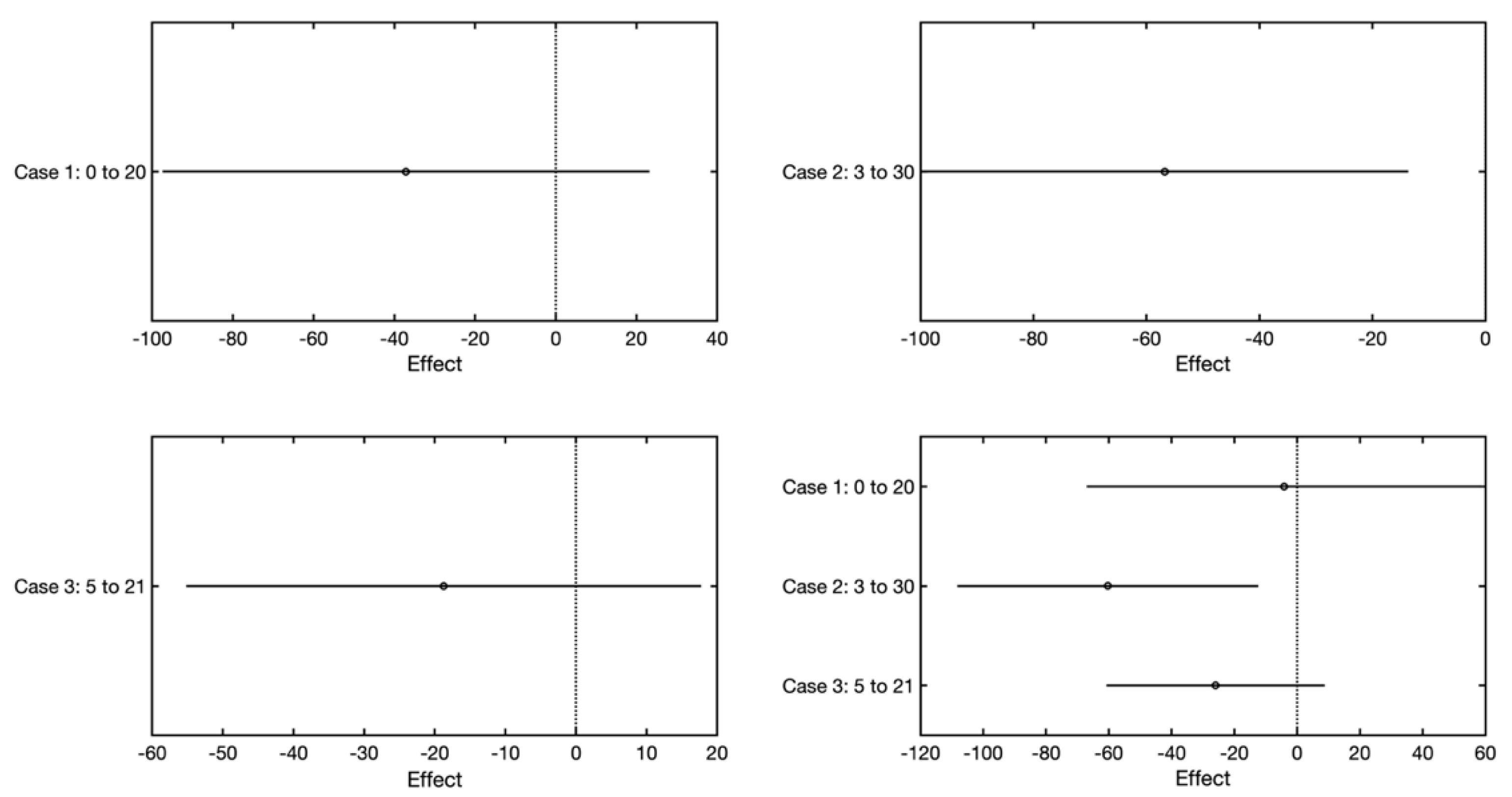
The Case 1, Case 2, and Case 3 variables are available in the dataset; these represent the numbers of use cases divided according to complexity, which is governed by the number of steps. As in the case of the actors, the effect of the individual use case types is also examined separately, followed by all the types together, with the last model examining the possible dependency of the total number of use cases on the size of the software system. Models are captured in which the number of use cases is used as an independent variable. From the analysis, it follows that only the Case 2 variable and the combination of the Case 1–3 variables has a weak ability to explain the dependent variable (11%). Individually, the Case 1 and 3 variables are not able to explain the dependent variable. This is also confirmed by the graph, which illustrates benefits (Figure 10), where averagely complex use cases (Case 2) show a small benefit. In the case of the other variables, no benefit is demonstrated (Figure 11).

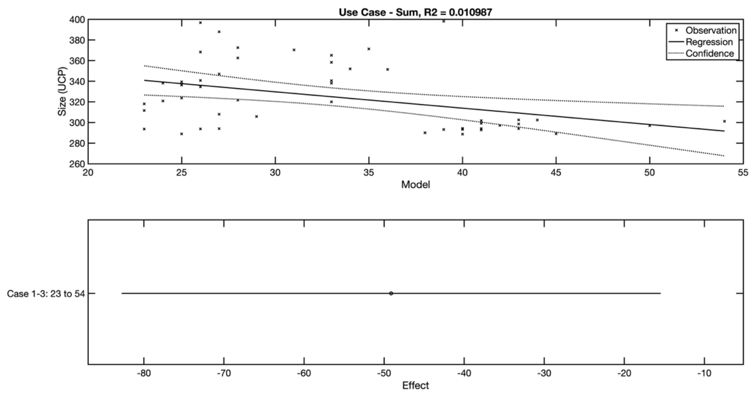
The last view is of a model that has the total number of use cases as an independent variable. In Figure 12, it is evident that the relationship between the total number of use cases and the size of the software system is also not strong.

4.3. Evaluation Criteria

The models’ evaluation uses criteria that are utilized for the evaluation of regression models, as well as criteria that are common in the area of software system size estimation. These include the mean absolute residual (MAR) Equation (1), the mean magnitude of relative error (MMRE) Equation (2), the number of projects with an error smaller than the entered value (PRED) Equation (3), the mean absolute percentage error (MAPE) Equation (4), the sum of squared errors (SSE) Equation (5), and the mean squared error (MSE) Equation (6).

$$\mathrm{MAR}=\frac{1}{n}{\displaystyle \sum }_{i=1}^n\left|y_i-\widehat{y_i}\right|$$

(1)

$$\mathrm{MMRE}=\frac{1}{n}{\displaystyle \sum }_{i=1}^n\frac{\left|y_i-\widehat{y_i}\right|}{y_i}$$

(2)

$$\mathrm{PRED}\left(\mathrm{l}\right)= \frac{1}{n}{\displaystyle \sum }_{i=1}^n\{\begin{array}{c}1 if \frac{\left|y_i-\widehat{y_i }\right|}{y_i}\le l\\ 0 if \frac{\left|y_i-\widehat{y_i }\right|}{y_i}>l\end{array}$$

(3)

$$\mathrm{MAPE}= \frac{1}{n}{\displaystyle \sum }_{i=1}^n\frac{\left|y_i-\widehat{y_i}\right|}{y_i} \times 100$$

(4)

$$\mathrm{SSE}= {\displaystyle \sum }_{i=1}^n{\left(y_i-\widehat{y_i}\right)}_i^2$$

(5)

$$\mathrm{MSE}= \frac{1}{n}{\displaystyle \sum }_{i=1}^n{\left(y_i-\widehat{y_i}\right)}_i^2$$

(6)

where n is the number of observations, $y_i$ is the real size in UCP points, $\widehat{y_i}$ is the estimated value, and $l$ is the error boundary as a percentage. If $l=0.25$ is considered, then a number for which is an estimate error smaller than or equal to 25% of the real size in UCP points is counted.

The adjusted coefficient of determination ($R_{Adj}^2)$ shows Equation (7) how the selected set of independent variables can explain the dependent variable. During the calculation, the number of observations and the number of independent variables are taken into consideration. The value $R_{Adj}^2$ can acquire a value between 0 and 1.

$$R_{Adj}^2= 1-\left(1-R^2\right)\times \frac{n-1}{n-k-1}$$

(7)

where $R^2$ is the coefficient of determination, $k$ is the number of independent variables, and $n$ is the number of observations.

Two graphic approaches are also utilized here. The first of these is the utilization of regression error characteristic curves [43]. The second is the graphic representation of the effects of changing independent variables [13] on the trained models.

5. Results

The AUCSE method was proposed to simplify a software size estimate based on the use case model. In this section, results are shown and discussed.

It was previously demonstrated that the direct dependency of variables on the size of the system is weak. That is why, in order to find the most suitable combination of variables, the stepwise regression method, as previously described, is used.

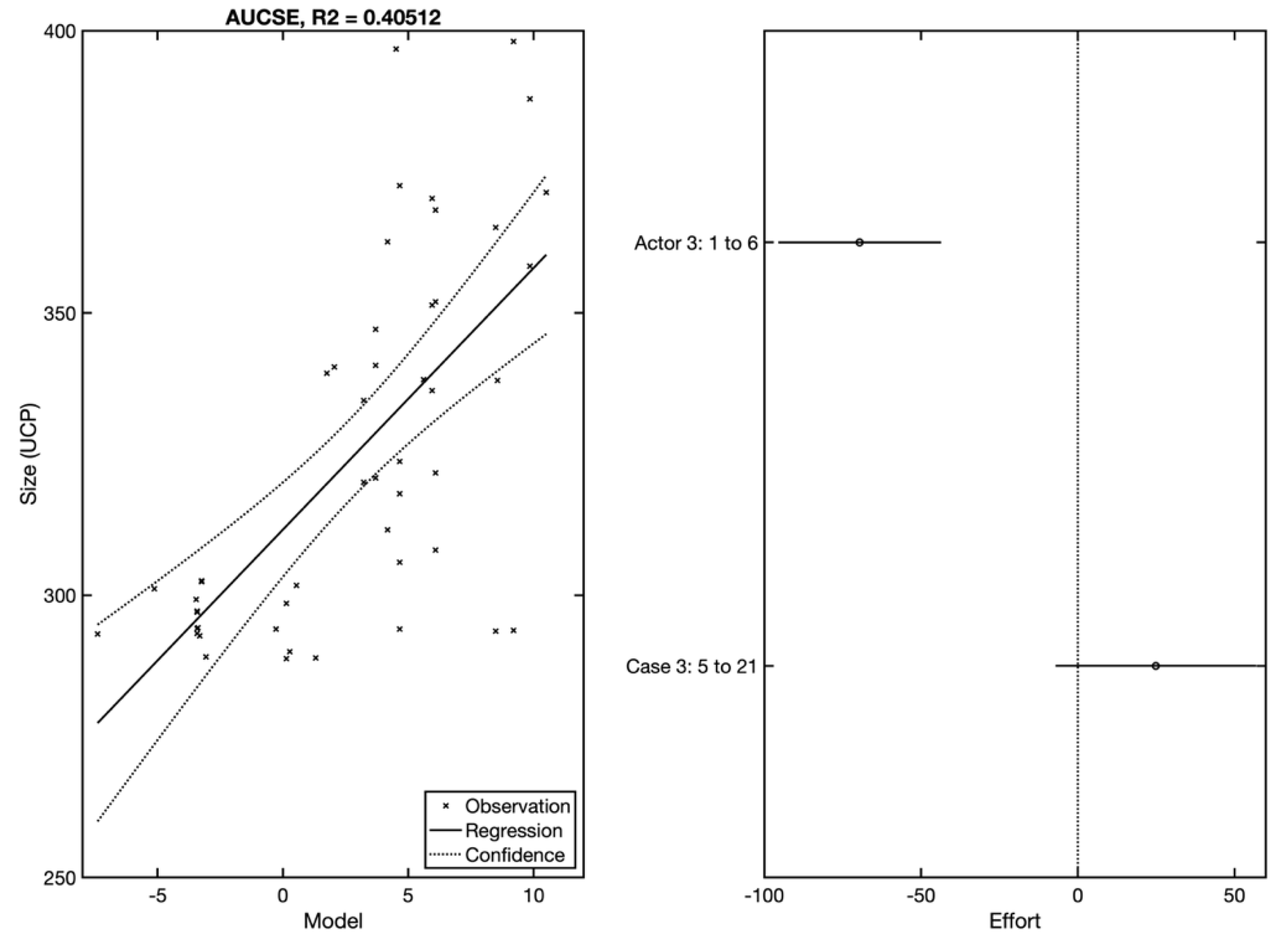
The proposed AUCSE model is based on the utilization of independent variables, which describe the number of actors (Actor 1–3) and the number of use cases (Case 1–3). When adding and removing independent variables, the value of the adjusted $R^2$ is monitored, whereby the objective is its maximization while fulfilling other, previously described conditions. The following figure (Figure 13) illustrates an AUCSE method that was created in the training part of Dataset DS, as well as a graphic representation of the benefit of selected independent variables. This model can be described using Equation (8).

$$UCP ~ 1 + Actor 3\ast Case 3$$

(8)

The model contains the constant component and all the interactions between the independent Actor 3 and Case 3 variables. An ability to explain more than 40% of the variability of the dependent variable was achieved.

The model’s estimating abilities were verified on the testing part of DS. If we compare the achieved results with the standard UCP approach, we can say that a significant increase in accuracy occurred (

Table 2. Comparison of UCP and AUCSE.

Model	MAR	MMRE	PRED (0.25)	MAPE	SSE	MSE
UCP	72.16	0.27	0.47	27.36	293,820	13,992
AUCSE	17.9	0.05	1	5.90	13,643	649.68

). The mean absolute residual (MAR) decreased by two-thirds, and the model is able to estimate all of the observations in the testing part with an error smaller than 25%. In contrast, the UCP method is only able to estimate 47% of projects with an error of 25%. From the graph (Figure 14), it also follows that AUCSE with stepwise regression allows for the estimation of more than 80% of observations with an error smaller than 10%.

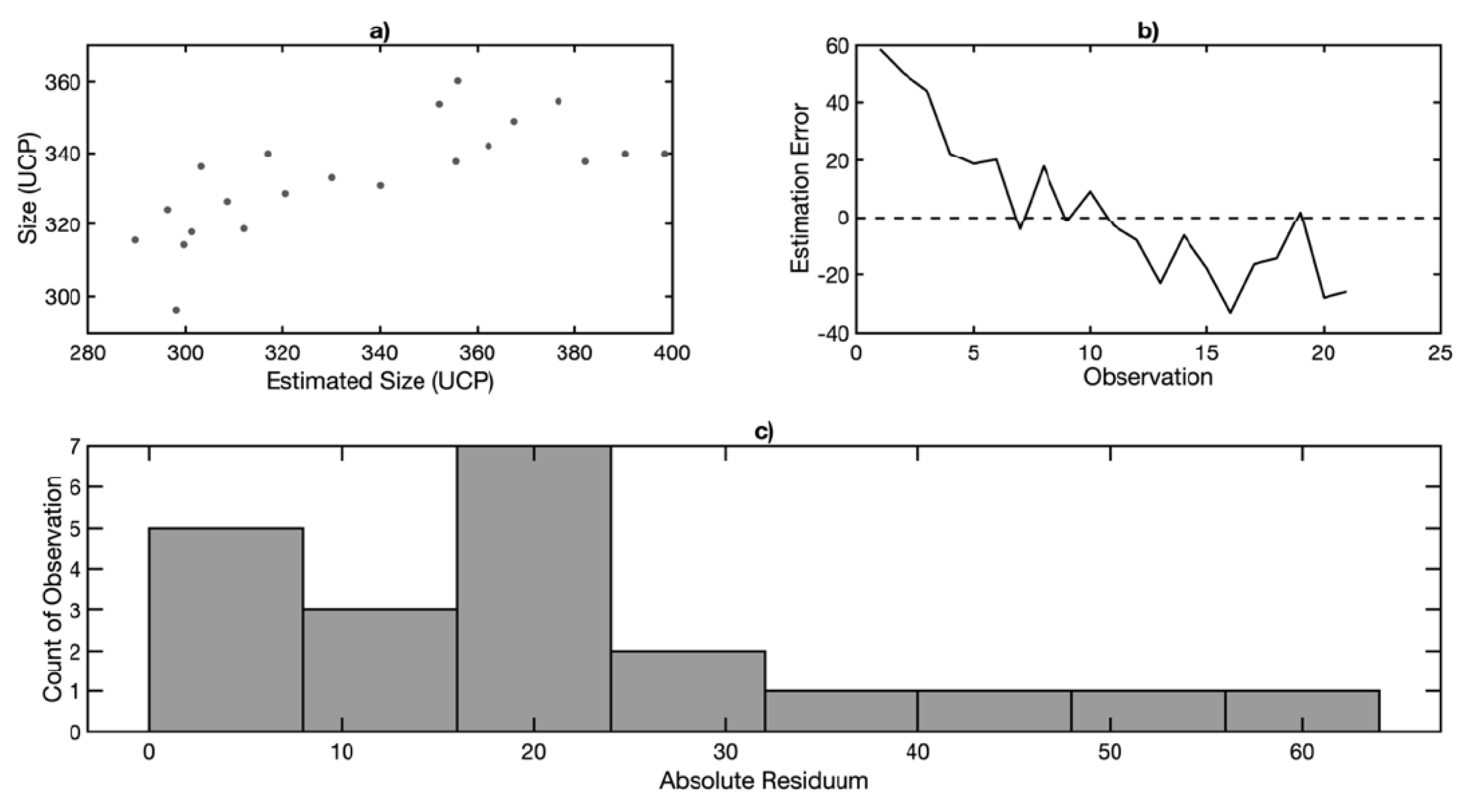
Therefore, it can be stated that the AUCSE achieves an estimation accuracy that is acceptable in practice. An overall view of estimation errors is offered by the graph of errors (Figure 15), which captures the relationship between the real and estimated size (a), the development of errors for individual observations (b), and the histogram of absolute residuals (c).

5.1. Comparison of Linear Regression Methods for Actors and Use Cases

When looking at the models themselves, they appear not to be completely suitable for estimation purposes. Of the linear regression methods, the model based on stepwise regression achieved the best results. This model utilizes the independent Actor 3 and Case 3 variables, i.e., actors and use cases with the highest complexity.

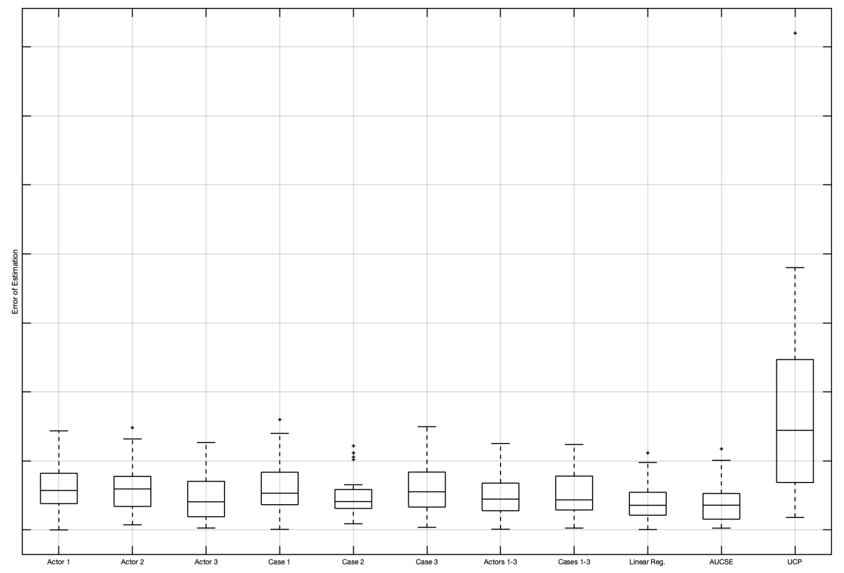
In Figure 16 and Figure 17, a comparison of the methods according to the selected criteria is captured. All of the criteria confirm the selection of the model based on stepwise regression, which leads to the highest increase in accuracy (by more than 90%) compared to UCP.

Table 3. Comparison of AUCSE to other model variants.

Model	MAR	MMRE	PRED (0.25)	MAPE	SSE	MSE
UCP	72.16	0.27	0.47	27.36	293,820	13,992
Actor 1	28.60	0.08	1	8.80	27,177	1294
Actor 2	29.66	0.08	1	8.83	27,000	1286
Actor 3	20.37	0.07	1	7.28	19,181	1285
Case 1	26.55	0.09	1	9.25	29,910	1424
Case 2	20.55	0.09	1	7.25	18,780	894
Case 3	27.61	0.08	1	8.87	28,243	1344
Actors 1–3	22.32	0.07	1	7.37	19,322	920
Cases 1–3	21.77	0.07	1	7.83	21,689	1032
Linear regression	17.8	0.06	1	6.30	14,408	686.10
AUCSE	17.9	0.05	1	5.90	13,643	649.68

shows a specific comparison of criteria values for each of the tested linear regression models as defined in this paper.

5.2. Comparison of AUCSE and Selected Methods Based on Use Case Points

In

Table 4. Comparison of AUCSE to methods based on UCP.

Model	MAR	MMRE	PRED (0.25)	MAPE	MSE
AUCSE	17.9	0.05	1	5.90	649.68
RegA [26]	n/a	0.34	0.37	n/a	n/a
RegB [28]	n/a	0.57	0.29	n/a	n/a
StepR [23]	12.81	0.04	1	4.85	433.76
ANN [28]	n/a	0.49	0.29	n/a	n/a
MLP [26]	n/a	0.55	0.37	n/a	n/a
KM [29]	2.4	0.01	1	0.91	13.23
SC [29]	2.4	0.01	1	0.91	13.23
MW [29]	11.09	0. 05	1	5.94	474.63
UCP	72.16	0.27	0.47	27.36	13,992

, there is a comparison to methods, which were designed as an improvement and modification of the original UCP method. The AUCSE stands for the proposed method, and UCP stand for the original baseline method. Other models are adopted as were presented in original publications. RegA and RegB are log-transformed models, which represent improvements of the original UCP method. StepR is a stepwise regression that is one of the most promising regressions, because it can be used for derivation of the best performing model based on available data. ANN and MLP represent a neural network model. KM and SC represent k-means and spectral clustering in combination with StepR. Those can be understood as the most advanced improvements of original UCP. MW is a moving windows-based model, which is used in several publications, as a segmentation method, which understands newer projects (from a time point of view) as more relevant than older projects.

As can be seen from Table 4, the results of AUCSE are promising. There are methods based on UCP that provide slightly more accurate estimation, but when the simplicity of the AUCSE method is taken into account, than AUCSE is a more convenient solution. It can be expected that advanced tuning methods (clustering, moving windows) will improve AUCSE accuracy even more.

5.3. Threats to Validity

The limitation is of this study is related to dataset availability. There is no other dataset that may be used for method evaluation. There are some other datasets that deal with Use Case Points, but in those datasets, there is no information about actors and use cases structure. Therefore, larger datasets cannot be used for evaluation. The validity of the research was achieved by using a hold-out principle for creation testing and training datasets.

The construct validity includes a question regarding the size (UCP). The collected data including the total effort in person-hours and size (UCP) were obtained by revaluated size after the projects were completed. During the data collection process for the dataset (DS), the authors obtained copies of the use case diagrams for only some of the projects—the rest of the participants considered their use case models proprietary. Therefore, we were forced to rely on the information provided by those who were involved in preparing the data for the survey in the software companies [23]. For the set of projects for which use case models were available, there is still a risk that the use case scenarios and actors were improperly designed by the data donator.

6. Discussion and Conclusions

The effort to eliminate the effect of the inaccurate determination of UCP components led to the design of a model based on the number of actors and use cases (AUCSE). Therefore, only variables based directly on the use case model—number of actors and number of use cases—were used as independent variables. The Actor 1–3 and Case 1–3 variables were used. The use of these independent variables, combined with stepwise regression, led to a very significant reduction in errors when estimating the size of software systems compared to UCP.

The aforementioned process achieves a high estimation accuracy and can be recommended as a system size estimation model. The processing of this model consists only of an analysis of the number of actors and use cases.

Results are broadly discussed in the Results section, in which the comparison to other methods is presented (Table 3 and Table 4). As can be seen, the AUCSE was compared to methods RegA [26], RegB [28], StepR [23], ANN [28], MLP [26], KM [29], SC [29], MW [29], and UCP. The AUCSE has advantages in simplicity and in accuracy. Only the SC method brings better results, but it has a more complex method. Moreover, all methods that are based on UCP (UCP components including TCF and ECF are needed) are sensitive to UCP estimator experience. The presented UCP modification allows us to minimize this influence. AUCSE excels in that only the use case model is needed for fast and accurate estimation. The estimation accuracy of AUCSE may be influenced by the use case model stage; early-stage models may influence estimation accuracy. To avoid this risk, the AUCSE model is based on stepwise regression, and the use of the local data can be recommended.

When assessing RQ1, it can be deduced that the effect of the number of actors and use cases has been demonstrated. The most accurate results were achieved with the application of stepwise regression, where the independent Actor 3 and Case 3 variables were used. The correlation of the other variables was not significant. As a result, they have little effect (positive or negative) on the accuracy of the estimate. This is also the reason why linear regression, too, achieves an interesting accuracy.

From the analysis, it also follows that in response to RQ2, it can be said that the proposed AUCSE approach leads to a significant increase in estimate accuracy when compared to the UCP method. It is necessary at this point to also emphasize the simplification of the determination of the independent variable values, which increases the practical applicability of the presented AUCSE method.

When an AUCSE is compared to various modifications of the original UCP method (Table 4), it can be seen that AUCSE provides promising results. Advanced UCP modification (SC) provides a more accurate estimation. When the simplicity of AUCSE is taken into account for industry practice, the AUCSE is the best option. The approach that is used is designed for both normal-scale and large-scale projects. The advantage of AUCSE compared to the SC approach can be seen in the fact that all actors or use cases are evaluated according to complexity. The number of actors and mainly use cases depends on project size, so a large-scale project is handled in the same way as a small one.

In future research, attention will be devoted to further increasing the accuracy of the AUCSE method using clustering algorithms [44]. Moreover, it will include the testing of window functions [29] and a detailed comparison with selected methods, which can be used for UCP method tuning. The last but not least aspect that will be under further investigation will be the measurement of the AUCSE accuracy according the project size. In the used dataset, the mean size was approximately 300 UCP (for data provider D1, it was 360 UCP); therefore, in the future, the effectivity and accuracy of the AUCSE method for different project sizes (especially for large-size projects) will be investigated.