
Planning and Research of Distribution Feeder Automation with Decentralized Power Supply


Abstract
1. Introduction
2. Reconfiguration Problems
2.1. Distributed Generation Characteristics
2.2. Feeder Reconfiguration Constraints
2.2.1. Feeder Current Constraints
2.2.2. Voltage Variation
2.2.3. Reverse Power Limit
2.2.4. Radial Network
3. Optimal Algorithm Math Models
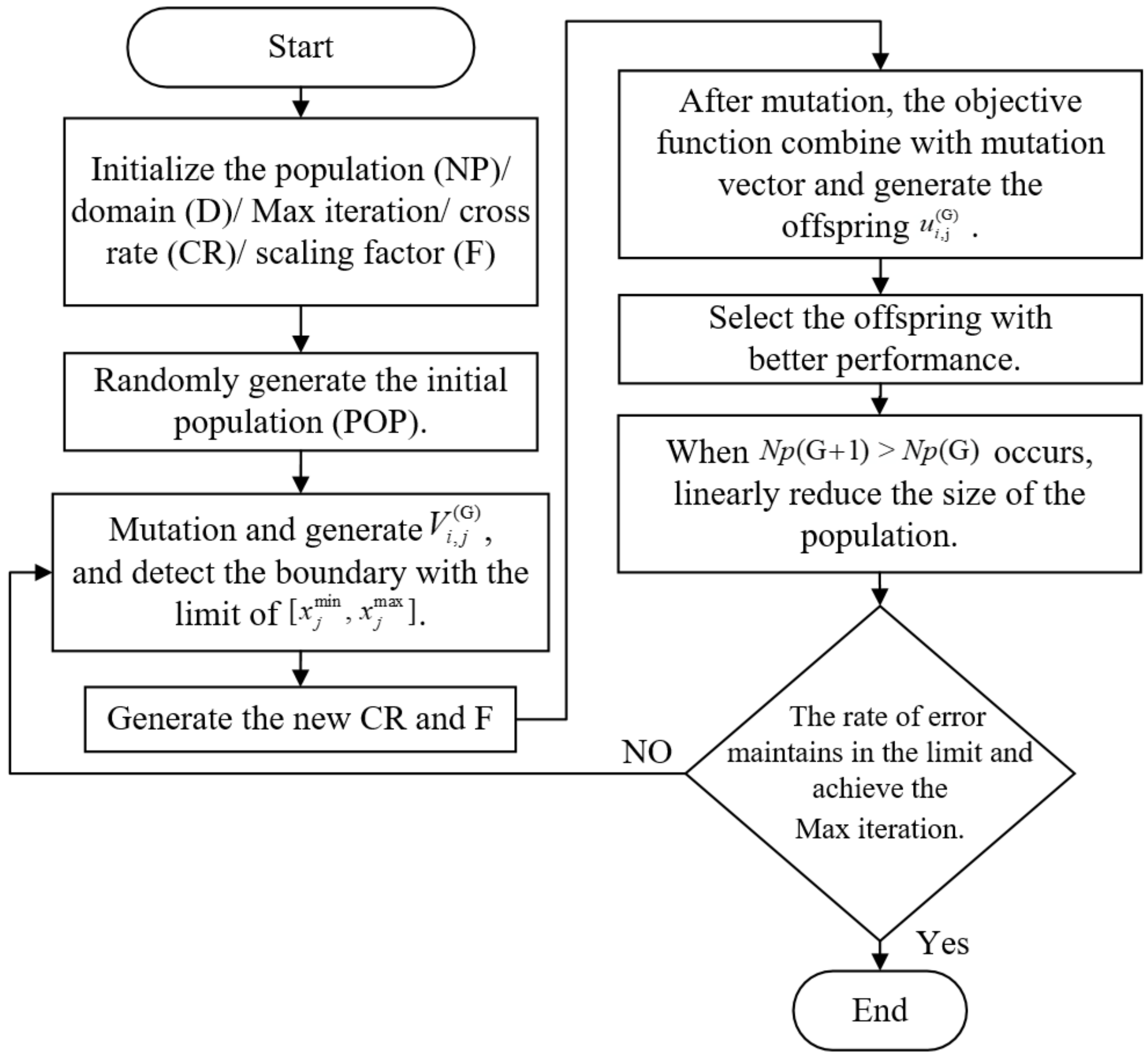
3.1. L-SHADE Optimal Algorithm
3.1.1. Initialize Population
3.1.2. Mutation
3.1.3. Parameter Adaption
3.1.4. Reconfiguration (Crossover)
3.1.5. Selection
3.1.6. Linear Population Size Reduction Technique
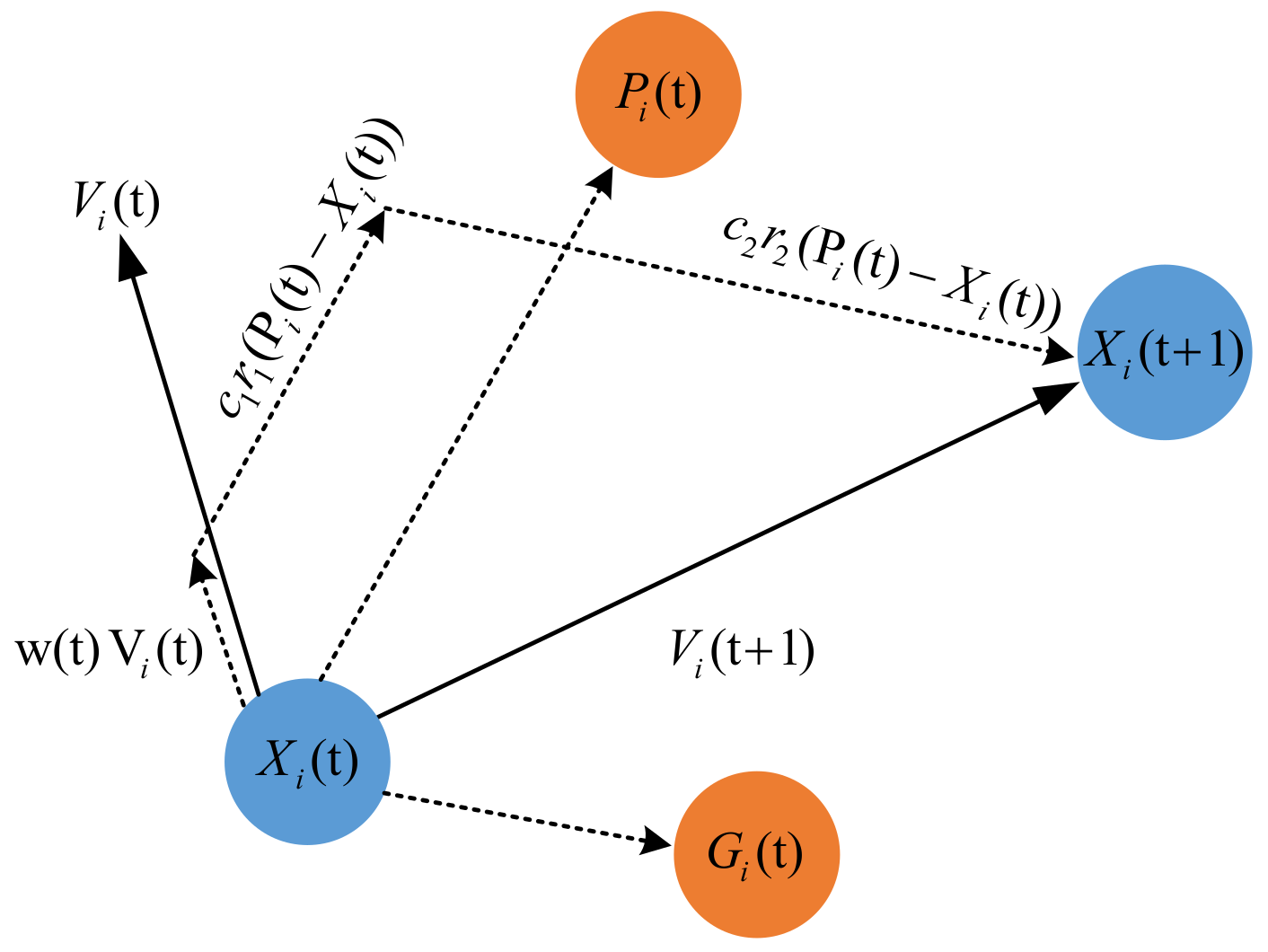
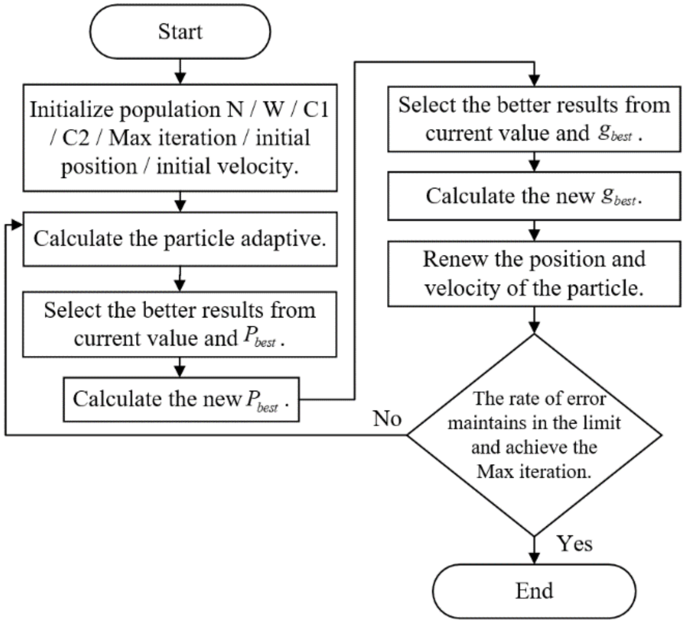
3.2. PSO Optimal Algorithm
3.3. Objective Function
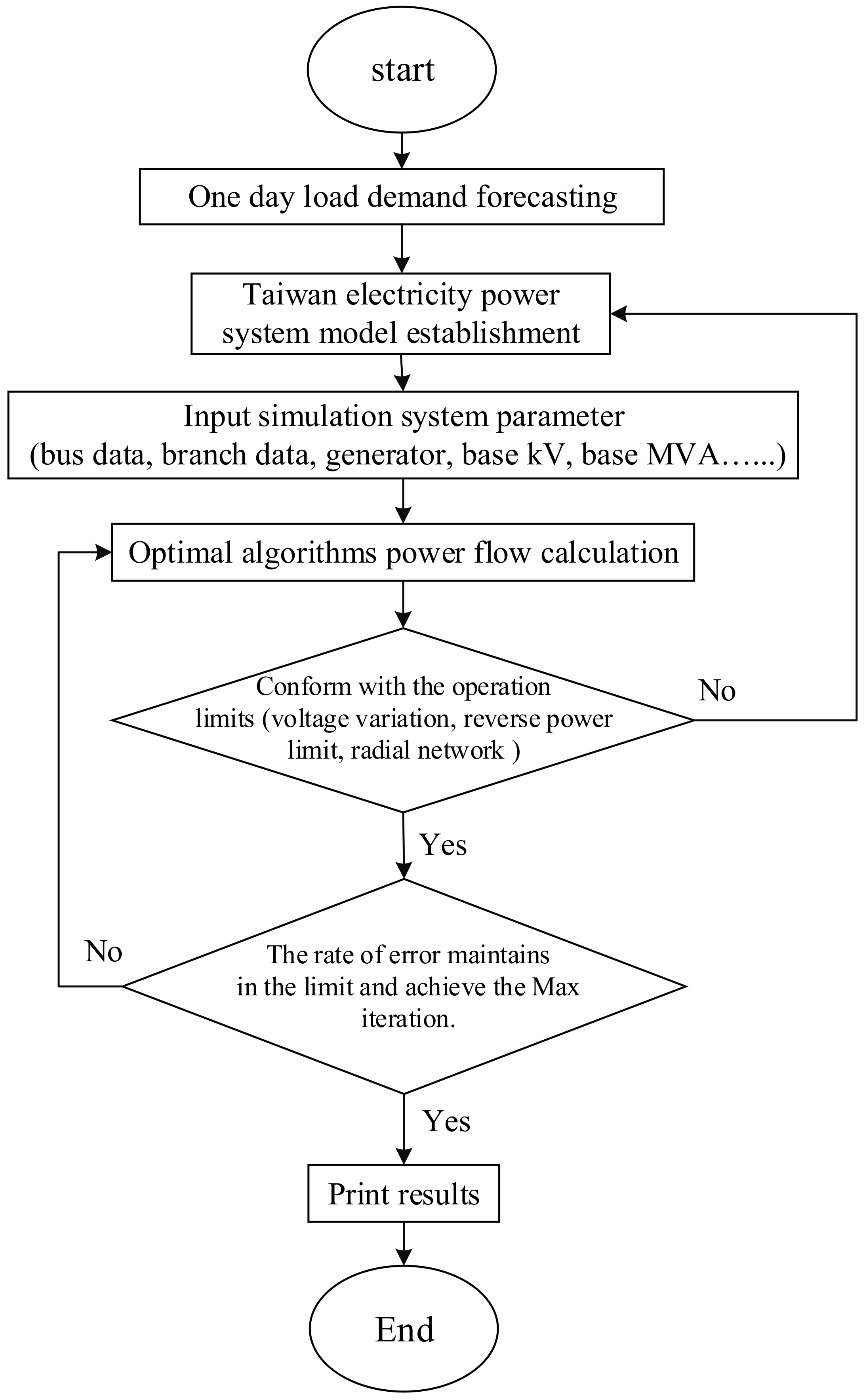
4. Case Study
4.1. System Parameter Definition
4.2. Optimal Reconfiguration Analysis
4.2.1. IEEE 33 System Background
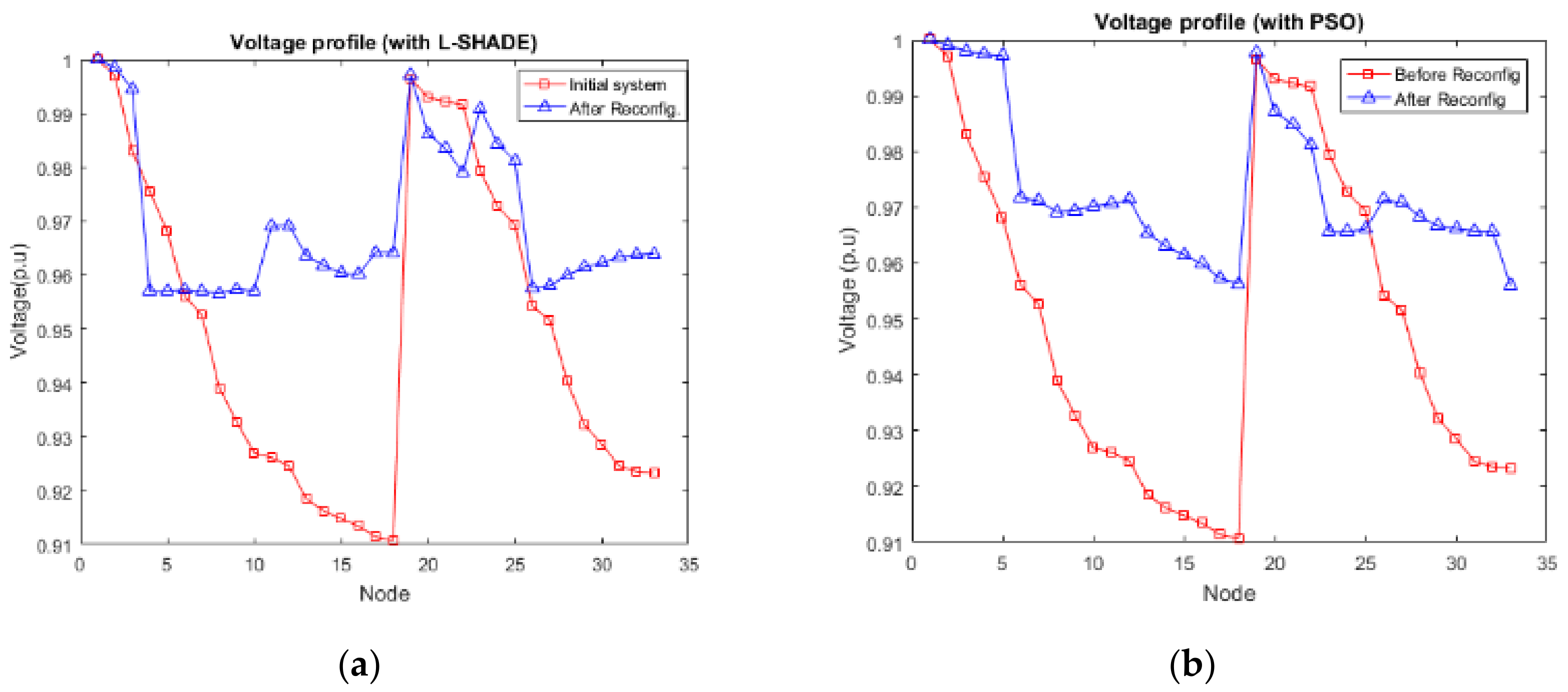
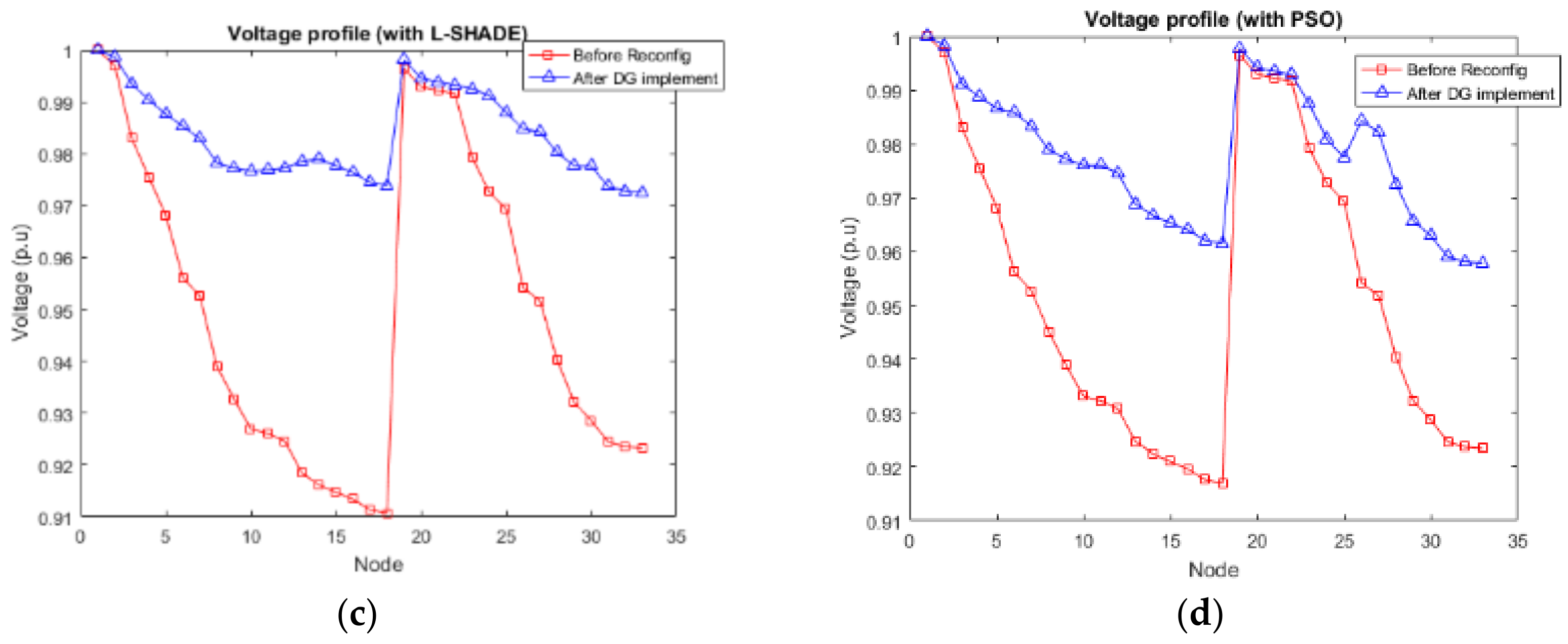
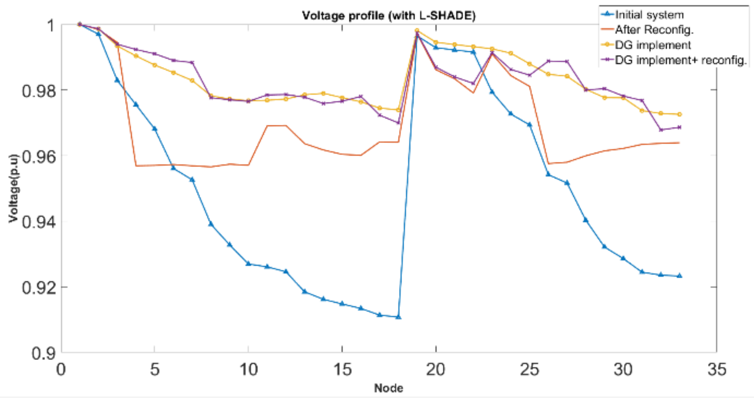
4.2.2. IEEE 33 Feeder Reconfiguration
4.3. Impact by Load Variation to the Feeder Switch
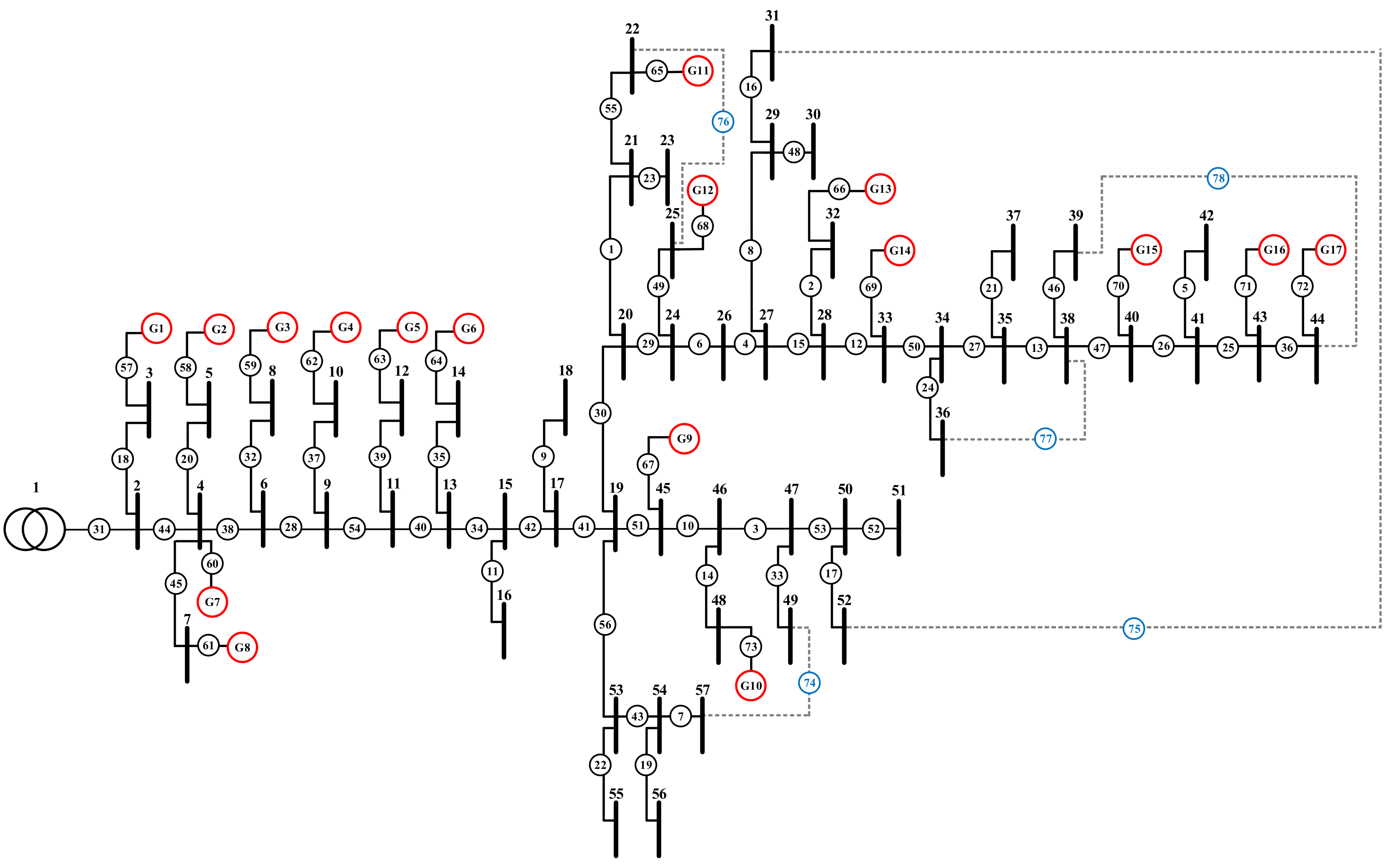
4.3.1. Taiwan Case 1 System Background
4.3.2. Taiwan Case 1 Feeder Reconfiguration
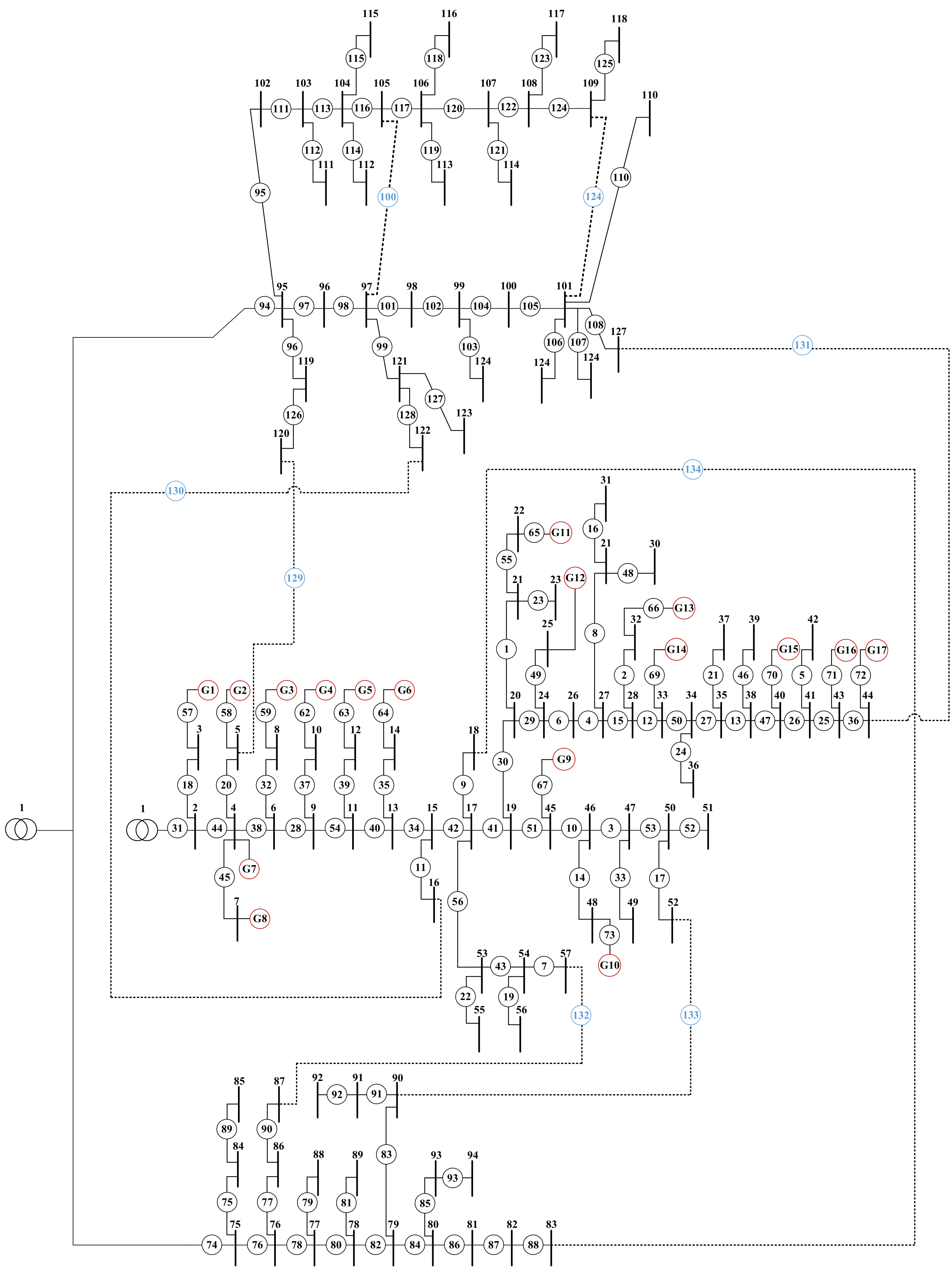
4.3.3. Taiwan Case 2 System Background
4.3.4. Taiwan Case 2 Feeder Reconfiguration
4.3.5. Reconfiguration Considering the Operation Frequency
5. Conclusions
Author Contributions
Funding
Acknowledgments
Conflicts of Interest
Nomenclature
| Pt | power generation per square meter |
| SSR | amount of irradiance observed by the satellite |
| PV panel transformation efficiency | |
| current between bus i and bus i + 1 | |
| , | voltage at ends of the feeder |
| resistance of the feeder | |
| reactance of the feeder | |
| current variation which passes through the feeder | |
| voltage difference between the two busses | |
| radial feeder after feeder reconfiguration | |
| combination of all types of radial feeder | |
| NP | population size |
| D | dimension |
| F | scaling factor |
| G | the Gth generation |
| CR | cross rate |
| learning factor | |
| NFE | number of fitness evaluations |
| best position of individual particle | |
| best position of current swarm particles | |
| maximum iteration times | |
| weight | |
| switch condition of the branch | |
| feeder branch resistance | |
| feeder branch active power | |
| feeder branch reactive power | |
| voltage on the feeder | |
| SHADE | Successful history-based adaptive differential evolution |
| L-SHADE | SHADE with linear population size reduction |
| PSO | particle swarm optimization |
| DG | Distributed generator |
| DE | Differential evolution |
| PV | Photovoltaic |
References
- Turan, G. Electric Power Distribution System Engineering; McGraw-Hill: New York, NY, USA, 1986; pp. 174–187. [Google Scholar]
- Settembrini, R.C.; Fisher, J.R.; Hudak, N.E. Reliability and Quality Comparisons of Electric Power Distribution Systems. In Proceedings of the 1991 IEEE Power Engineering Society Transmission and Distribution Conference, Dallas, TX, USA, 22–27 September 1991; pp. 704–712. [Google Scholar]
- Nasir, M.N.M.; Shahrin, N.M.; Bohari, Z.H.; Sulaima, M.F.; Hassan, M.Y. A Distribution Network Reconfiguration based on PSO: Considering DGs sizing and allocation evaluation for voltage profile improvement. In Proceedings of the 2014 IEEE Student Conference on Research and Development IEEE, Batu Ferringhi, Malaysia, 16–17 December 2014; pp. 1–6. [Google Scholar]
- Montoya, D.P.; Ramirez, J.M. Reconfiguration and optimal capacitor placement for losses reduction. In Proceedings of the 2012 Sixth IEEE/PES Transmission and Distribution: Latin America Conference and Exposition (T&D-LA) IEEE, Montevideo, Uruguay, 3–5 September 2012; pp. 1–6. [Google Scholar]
- Sedighizadeh, M.; Dakhem, M.; Sarvi, M. Optimal Reconfiguration and Capacitor Placement for Power Loss Reduction of Distribution System Using Improved Binary Particle Swarm Optimization. Int. J. Energy Environ. Eng. 2014, 5, 73. [Google Scholar] [CrossRef]
- Amin Heidari, M. Optimal Network Reconfiguration in Distribution System for Loss Reduction and Voltage-Profile Im-provement using Hybrid Algorithm of PSO and ACO. CIRED - Open Access Proc. J. 2017, 1, 2458–2461. [Google Scholar] [CrossRef]
- Muhammad, M.A.; Mokhlis, H.; Naidu, K.; Amin, A.; Franco, J.F.; Othman, M. Distribution Network Planning En-hancement via Network Reconfiguration and DG Integration Using Dataset Approach and Water Cycle Algorithm. J. Mod. Power Syst. Clean Energy 2020, 8, 86–93. [Google Scholar] [CrossRef]
- Azizivahed, A.; Narimani, H.; Fathi, M.; Naderi, E.; Safapour, H.R.; Narimani, M.R. Multi-objective dynamic distribution feeder reconfiguration in automated distribution systems. Energy 2018, 147, 896–914. [Google Scholar] [CrossRef]
- Li, Y.; Feng, B.; Li, G.; Qi, J.; Zhao, D.; Mu, Y. Optimal distributed generation planning in active distribution networks considering integration of energy storage. Appl. Energy 2018, 210, 1073–1081. [Google Scholar] [CrossRef]
- Kirkpatrick, S.; Gelatt, C.D., Jr.; Vecchi, M.P. Optimization by Simulated Annealing. Science 1983, 220, 671–680. [Google Scholar] [CrossRef] [PubMed]
- Martí, R.; Laguna, M.; Glover, F. Principles of Tabu Search. Veh. Netw. 2007, 23, 34–47. [Google Scholar] [CrossRef]
- Storn, R.; Price, K. Differential Evolution–A Simple and Efficient Heuristic for global Optimization over Continuous Spaces. J. Glob. Optim. 1997, 11, 341–359. [Google Scholar] [CrossRef]
- Dorigo, M.; Di Caro, G. Ant colony optimization: A new meta-heuristic. In Proceedings of the 1999 Congress on Evolutionary Computation-CEC99 (Cat. No. 99TH8406), Washington, DC, USA, 6–9 July 1999; Volume 2, pp. 1470–1477. [Google Scholar]
- Kennedy, J.; Eberhart, R. Particle swarm optimization. In Proceedings of the ICNN’95-International Conference on Neural Networks, Perth, WA, Australia, 27 November–1 December 1995; Volume 4, pp. 1942–1948. [Google Scholar] [CrossRef]
- Geem, Z.W.; Kim, J.H.; Loganathan, G. A New Heuristic Optimization Algorithm: Harmony Search. Simulation 2001, 76, 60–68. [Google Scholar] [CrossRef]
- Karaboga, D. An Idea Based On Honey Nee Swarm for Numerical Optimization; Erciyes University, Engineering Faculty: Kayseri, Turkey, October 2005; TECHNICAL REPORT-TR06. [Google Scholar]
- Biswas, P.P.; Suganthan, P.; Amaratunga, G.A.J. Optimal placement of wind turbines in a windfarm using L-SHADE algorithm. In Proceedings of the 2017 IEEE Congress on Evolutionary Computation (CEC), San Sebastian, Spain, 5–8 June 2017; pp. 83–88. [Google Scholar]
- Biswas, P.P.; Suganthan, P.; Amaratunga, G.A. Minimizing harmonic distortion in power system with optimal design of hybrid active power filter using differential evolution. Appl. Soft Comput. 2017, 61, 486–496. [Google Scholar] [CrossRef]
- Tanabe, R.; Fukunaga, A. Success-history based parameter adaptation for Differential Evolution. In Proceedings of the 2013 IEEE Congress on Evolutionary Computation, Cancun, Mexico, 20–23 June 2013; pp. 71–78. [Google Scholar]
- Tanabe, R.; Fukunaga, A.S. Improving the search performance of SHADE using linear population size reduction. In Proceedings of the 2014 IEEE Congress on Evolutionary Computation (CEC), Beijing, China, 6–11 July 2014; pp. 1658–1665. [Google Scholar]
- Baran, M.; Wu, F. Network reconfiguration in distribution systems for loss reduction and load balancing. IEEE Trans. Power Deliv. 1989, 4, 1401–1407. [Google Scholar] [CrossRef]


| Challenge | Statements |
|---|---|
| Intermittent generation | Time of generation peak is different with peak of load demand so takes the shape of duck curve. |
| Generation non-smoothing | The severe variation easily makes system voltage and current unstable. |
| Lack of system inertial | In the severe power accident, generation equipment has no time to respond, and is then disconnected. |
| Fault current | The fault current comes from the main transformer and distributed generation will cause feeder breaker lack of breaking capacity and increase short current. |
| Power reverse transmission | Comparing with the single way of electricity transmission before, the multiple transmission ways will easily cause main transformer power reverse transmission. |
| Type | Wire Diameter | Tolerable Max Current | |
|---|---|---|---|
| Underground Cable | Main Feeder | 500 MCM | 600 A |
| Branch | #1 AWG | 200 A | |
| Overhead lines | Main Feeder | 477 MCM | 590 A |
| Branch | #2 AWG | 165 A | |
| System | IEEE 33 [21] | Taiwan Case 1 System | Taiwan Case 2 System |
|---|---|---|---|
| Apparent power (MVA) | 100 | 25 | 25 |
| System voltage (kV) | 12.66 | 11.4 | 11.4 |
| Total of system load demand | 3715 kW + 2300 kvar | 1471.6 kW + 483.7 kvar (one-day average) | 2745.6 kW + 902.4 kvar (one-day average) |
| Branch number | 37 | 78 | 134 |
| Node number | 32 | 73 | 126 |
| Tie switch number | 5 | 5 | 8 |
| Scenario | Statement | L-SHADE | PSO |
|---|---|---|---|
| Before feeder reconfiguration (Initial System) | Tie switches | 33, 34, 35, 36, 37 | 33, 34, 35, 36, 37 |
| Power loss (kW) | 202.68 | 202.68 | |
| Power loss reduction percentage (%) | – | – | |
| Min voltage (bus number) | 0.91075 p.u. (18) | 0.91075 p.u. (18) | |
| After feeder reconfiguration | Tie switches | 3, 10, 16, 33, 37 | 5, 22, 32, 33, 34 |
| Power loss (kW) | 96.1344 | 150.6883 | |
| Power loss reduction percentage (%) | 52.57 | 25.65 | |
| Min voltage (bus number) | 0.95657 p.u. (8) | 0.95603 p.u. (33) | |
| After DG*3 implementation (keep initial system) | Tie switches | 33, 34, 35, 36, 37 | 33, 34, 35, 36, 37 |
| Power loss (kW) | 72.5447 | 90.7069 | |
| DG capacity (kW) (bus number) | 751 (14) 926 (24) 1021 (30) | 1220 (6) 650 (11) 200 (30) | |
| Power loss reduction percentage (%) | 64.21 | 55.25 | |
| Min voltage (bus number) | 0.9726 p.u. (33) | 0.9578 p.u. (33) |
| Scenario | Statement | Initial system | L-SHADE | PSO |
|---|---|---|---|---|
| After reconfiguration at 4:00 | Tie switches | 74, 75, 76, 77, 78 | 12, 17, 26, 30, 33 | 6, 10, 24, 30, 47 |
| Power loss (kW) | 13.4505 | 3.7289 | 12.3869 | |
| Power loss reduction percentage (%) | – | 72.2769% | 7.9075% | |
| Min voltage (bus number) | 0.9989 p.u. (18) | 0.9991 p.u. (49) | 0.9990 p.u. (18) | |
| After reconfiguration at 12:00 | Tie switches | 74, 75, 76, 77, 78 | 17, 33, 50, 76, 78 | 4, 24, 30, 33, 47 |
| Power loss (kW) | 9.9062 | 9.1997 | 9.8512 | |
| Power loss reduction percentage (%) | – | 7.1319% | 0.5552% | |
| Min voltage (bus number) | 0.9992 p.u. (18) | 0.9990 p.u. (49) | 0.9991 p.u. (18) | |
| After reconfiguration at 20:00 | Tie switches | 74, 75, 76, 77, 78 | 17, 24, 30, 33, 78 | 3, 6, 24, 26, 30 |
| Power loss (kW) | 31.5766 | 9.3244 | 31.9362 | |
| Power loss reduction percentage (%) | – | 70.4705% | −1.1388% | |
| Min voltage (bus number) | 0.9982 p.u. (18) | 0.9987 p.u. (49) | 0.9981 p.u. (18) |
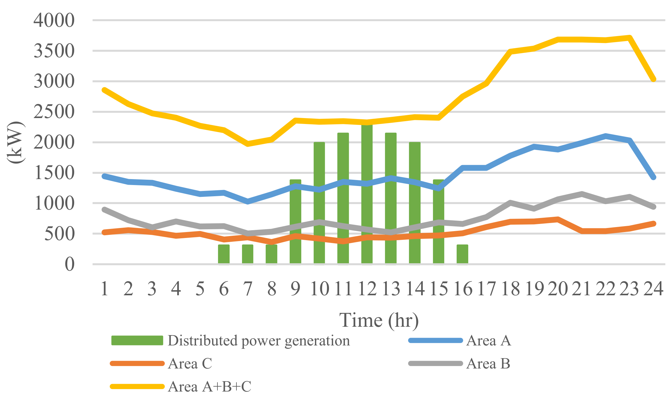
| System | Area A | Area B | Area C | Area A + B + C |
|---|---|---|---|---|
| Apparent power (MVA) | 25 | |||
| System voltage (kV) | 11.4 | |||
| Total of system load demand (one-day average) | 1471.6 kW + 483.7 kvar | 756.7 kW + 248.7 kvar | 517.3 kW + 170 kvar | 2745.6 kW + 902.4 kvar |
| Branch number | 73 | 35 | 20 | 134 |
| node number | 73 | 33 | 20 | 126 |
| DG number | 17 | 0 | 0 | 17 |
| Total DG capacity (kW) | 3057.7 | – | – | 3057.7 |
| Tie switch number | – | 2 | – | 8 |
| Time | Tie Switches Variation | |||||||
|---|---|---|---|---|---|---|---|---|
| Original system | 100 | 109 | 129 | 130 | 131 | 132 | 133 | 134 |
| 00:00 | 6 | 53 | 54 | 84 | 99 | 111 | 117 | 132 |
| 01:00 | 3 | 28 | 29 | 84 | 99 | 111 | 124 | 132 |
| 02:00 | 3 | 4 | 28 | 84 | 99 | 113 | 124 | 132 |
| 03:00 | 3 | 7 | 12 | 40 | 84 | 99 | 102 | 116 |
| 04:00 | 3 | 7 | 40 | 50 | 84 | 99 | 116 | 117 |
| 05:00 | 28 | 50 | 51 | 84 | 99 | 104 | 116 | 132 |
| 06:00 | 15 | 34 | 53 | 84 | 99 | 116 | 120 | 132 |
| 07:00 | 3 | 29 | 40 | 84 | 99 | 111 | 124 | 132 |
| 08:00 | 3 | 28 | 50 | 77 | 84 | 99 | 111 | 117 |
| 09:00 | 10 | 12 | 58 | 82 | 84 | 99 | 116 | 124 |
| 10:00 | 12 | 51 | 54 | 77 | 84 | 99 | 101 | 111 |
| 11:00 | 3 | 29 | 54 | 84 | 99 | 113 | 120 | 132 |
| 12:00 | 10 | 30 | 58 | 82 | 84 | 99 | 111 | 120 |
| 13:00 | 15 | 51 | 58 | 84 | 90 | 99 | 113 | 124 |
| 14:00 | 3 | 50 | 54 | 84 | 99 | 111 | 117 | 132 |
| 15:00 | 10 | 50 | 54 | 80 | 84 | 99 | 113 | 117 |
| 16:00 | 41 | 51 | 78 | 84 | 99 | 113 | 117 | 129 |
| 17:00 | 15 | 20 | 51 | 80 | 84 | 99 | 113 | 124 |
| 18:00 | 34 | 50 | 53 | 84 | 90 | 99 | 113 | 124 |
| 19:00 | 6 | 20 | 51 | 82 | 84 | 99 | 116 | 120 |
| 20:00 | 4 | 28 | 53 | 84 | 99 | 113 | 117 | 132 |
| 21:00 | 3 | 15 | 34 | 77 | 84 | 99 | 116 | 120 |
| 22:00 | 41 | 51 | 54 | 78 | 84 | 99 | 116 | 124 |
| 23:00 | 12 | 38 | 51 | 84 | 99 | 105 | 113 | 132 |
| Switch number | 3 | 51 | 54 | 111 | 113 | 117 | 124 | 132 |
| Operation frequency | 10 | 12 | 8 | 10 | 12 | 10 | 12 | 11 |
| Time | Tie Switches Variation | |||||||
|---|---|---|---|---|---|---|---|---|
| Original system | 100 | 109 | 129 | 130 | 131 | 132 | 133 | 134 |
| 00:00 | 3 | 13 | 34 | 84 | 99 | 113 | 122 | 132 |
| 01:00 | 7 | 13 | 34 | 53 | 84 | 99 | 113 | 122 |
| 02:00 | 3 | 13 | 34 | 84 | 99 | 111 | 124 | 132 |
| 03:00 | 3 | 7 | 13 | 34 | 84 | 99 | 111 | 124 |
| 04:00 | 13 | 34 | 83 | 84 | 99 | 113 | 124 | 132 |
| 05:00 | 34 | 50 | 53 | 84 | 99 | 113 | 122 | 132 |
| 06:00 | 3 | 7 | 13 | 34 | 84 | 99 | 113 | 122 |
| 07:00 | 7 | 13 | 34 | 53 | 84 | 99 | 113 | 124 |
| 08:00 | 7 | 13 | 34 | 53 | 84 | 95 | 99 | 124 |
| 09:00 | 3 | 7 | 34 | 50 | 84 | 95 | 99 | 124 |
| 10:00 | 13 | 34 | 83 | 84 | 95 | 99 | 122 | 132 |
| 11:00 | 3 | 7 | 13 | 34 | 84 | 99 | 111 | 124 |
| 12:00 | 13 | 34 | 53 | 84 | 95 | 99 | 122 | 132 |
| 13:00 | 7 | 34 | 50 | 53 | 84 | 99 | 113 | 124 |
| 14:00 | 3 | 7 | 13 | 34 | 84 | 99 | 113 | 122 |
| 15:00 | 7 | 34 | 50 | 83 | 84 | 99 | 113 | 124 |
| 16:00 | 13 | 34 | 53 | 84 | 99 | 111 | 122 | 132 |
| 17:00 | 10 | 34 | 50 | 84 | 99 | 113 | 122 | 132 |
| 18:00 | 3 | 13 | 34 | 84 | 99 | 113 | 124 | 132 |
| 19:00 | 13 | 34 | 53 | 84 | 99 | 113 | 124 | 132 |
| 20:00 | 13 | 34 | 53 | 84 | 95 | 99 | 124 | 132 |
| 21:00 | 7 | 34 | 50 | 53 | 84 | 99 | 113 | 124 |
| 22:00 | 3 | 7 | 13 | 34 | 84 | 95 | 99 | 124 |
| 23:00 | 34 | 50 | 83 | 84 | 95 | 99 | 122 | 132 |
| Switch number | 3 | 7 | 13 | 50 | 53 | 122 | 124 | 132 |
| Operation frequency | 14 | 12 | 14 | 14 | 12 | 13 | 12 | 13 |
Publisher’s Note: MDPI stays neutral with regard to jurisdictional claims in published maps and institutional affiliations. |
© 2021 by the authors. Licensee MDPI, Basel, Switzerland. This article is an open access article distributed under the terms and conditions of the Creative Commons Attribution (CC BY) license (http://creativecommons.org/licenses/by/4.0/).
Share and Cite
Huang, Y.-C.; Chang, W.-C.; Hsu, H.; Kuo, C.-C. Planning and Research of Distribution Feeder Automation with Decentralized Power Supply. Electronics 2021, 10, 362. https://doi.org/10.3390/electronics10030362
Huang Y-C, Chang W-C, Hsu H, Kuo C-C. Planning and Research of Distribution Feeder Automation with Decentralized Power Supply. Electronics. 2021; 10(3):362. https://doi.org/10.3390/electronics10030362
Chicago/Turabian StyleHuang, Yen-Chih, Wen-Ching Chang, Hsuan Hsu, and Cheng-Chien Kuo. 2021. "Planning and Research of Distribution Feeder Automation with Decentralized Power Supply" Electronics 10, no. 3: 362. https://doi.org/10.3390/electronics10030362
APA StyleHuang, Y.-C., Chang, W.-C., Hsu, H., & Kuo, C.-C. (2021). Planning and Research of Distribution Feeder Automation with Decentralized Power Supply. Electronics, 10(3), 362. https://doi.org/10.3390/electronics10030362