Abstract
Guidance, navigation, and control system design is, undoubtedly, one of the most relevant issues in any type of unmanned aerial vehicle, especially in the case of military missions. This task needs to be performed in the most efficient way possible, which involves trying to satisfy a set of requirements that are sometimes in opposition. The purpose of this article was to compare two different control strategies in conjunction with a path-planning and guidance system with the objective of completing military missions in the most satisfactory way. For this purpose, a novel dynamic trajectory-planning algorithm is employed, which can obtain an appropriate trajectory by analyzing the environment as a discrete 3D adaptive mesh and performs a softening process a posteriori. Moreover, two multivariable control techniques are proposed, i.e., the linear quadratic regulator and the model predictive control, which were designed to offer optimal responses in terms of stability and robustness.
1. Introduction
On the basis of several forecasts and predictions, the global market for unmanned aerial vehicles (UAVs) is predicted to grow quickly in future years. For instance, the integration of UAVs into the aerospace market of the United States is projected to represent an economic impact of USD 89.1 billion between 2015 and 2025 [1].
A wide variety of actions can be completed by UAVs in different scenarios [2], offering a huge versatility, while artificial intelligence (AI) is more and more frequently employed to enhance their autonomy [3]. Missions incorporate civilian (photography, environmental monitoring, extinguishing wildfires, etc.) and military (reconnaissance, surveillance, target acquisition, etc.) purposes [4,5,6,7].
One example of a military mission could be dropping bombs over an objective from an initial location, which is the purpose of the UAV proposed in this article. In this case, the selected aircraft is the F-86 Sabre [8,9], which was hypothetically flown without a pilot for the whole mission. Obviously, other unmanned combat air systems (UCASs) would be more suitable for this mission, such as the X-47B [10,11]. However, it is not easy to find precise information about the aerodynamic characteristics of these combat aircraft, which would allow the implementation of a dynamic nonlinear model for accurate simulations. In contrast, there is detailed information available regarding Sabre, which facilitates the elaboration of those precise nonlinear dynamical simulation models.
To accomplish any autonomous 3D flight, path planning and guidance, navigation, and control methodologies are employed. Path planning determines the flight trajectory that the UAV should follow to move from an initial point to a final one, avoiding obstacles during the route. By employing sensors like a global positioning system (GPS), inertial units, magnetometers, etc, as well as estimation algorithms like the Extended Kalman Filter [12], the navigation system calculates the actual position and velocity. The proposed trajectory along with the navigation information is computed by the guidance law to determine the main reference signals for the control algorithms. Finally, to ensure the desired motion of a UAV, appropriate control techniques that can determine the actuator signals at each time step are required.
The purpose of this work was to compare two optimal multivariable controllers—in particular, a linear quadratic regulator (LQR) and model predictive control (MPC)—for trajectory tracking in combat missions in which obstacles are averted and a blitz is performed. Hence, both control techniques’ behaviors were studied based on flight autonomy, reference following, obstacle avoidance, and bomb impact accuracy. The main goal is to discuss which is the most suitable alternative for this kind of mission using a realistic simulation environment. Additionally, in this comparative study, no landing or takeoff procedures were studied, since the objective consisted of evaluating the flying system’s performance during demanding maneuvers.
Figure 1 summarizes the global scheme implemented in this article for the comparative study of the MPC vs. LQR control techniques.

Figure 1.
Diagram of the technical procedure conducted in the article.
The autonomous flying system implemented in this article is composed of two fundamental blocks: path-planning algorithms and a guidance, navigation, and control (GNC) system.
1.1. Path Planning
There is a high diversity of options for implementing successful 3D path planning. Some algorithms are based on sampling fundamentals, with a deep analysis from a 2D perspective [13], but not in a 3D environment; other options are node-based algorithms, which are mathematical structures utilized to model pairwise relationships (structures with vertices and edges), and they have a final purpose of analyzing the cost of examining nodes to find the optimal path. Moreover, bio-inspired algorithms and mathematical models are widely employed, among other techniques [14].
The node-based approach was utilized herein. This type of algorithm presents various methodologies, such as Dijkstra’s algorithm [15], A* [16], D* [17], or Theta* [18]. Recently, this technique has been enhanced with modern learning machine methods [14].
Moreover, different planning possibilities have been presented: obstacle avoidance (static and/or dynamic), real-time processing (on- or offline), and optimization parameters (total distance, flight parameters, etc.). The flying system must be able to analyze any obstacle online, although, in order to simplify the problem, an offline static obstacle approach, which attempts to achieve the least demanding trajectory for a UAV, is typically selected.
Many obstacle analysis strategies have been implemented over the years, and have mainly utilized accurate sensors [19] or image processing [20,21]. Nevertheless, in this article, a more simple approach was created, since the obstacles in this approach are defined computationally from the beginning.
Adaptive cell decomposition (ACD) is a strong method for solving physical systems by means of partial differential equations, enabling refined complex 3D Cartesian geometry reconstructions. Consequently, an ACD is proposed in this article, in which the 3D space is decomposed and explored through recursive rewarding cost functions. Afterward, a 3D smooth path-planning algorithm is applied after the ACD in order to obtain a more achievable dynamic trajectory for the UAV during the mission through the introduction of gyration radii in each waypoint from the ACD route. In addition, a reference velocity profile is defined.
1.2. Guidance, Navigation, and Control
As mentioned before, GNC systems are applied to ensure appropriate management of any vehicle’s movement. First, the guidance function determines the commanded attitude based on the reference trajectory and the navigation information. Then, the control block applies the control actions needed by actuators to fulfill such commands, while stability is guaranteed [22].
In relation to these systems, there are different aspects that play a key role in ensuring the aircraft’s proper motion, such as position detection techniques [23] or hardware implementation [24], but only theoretical investigation is proposed in this article. Furthermore, the navigation problem has been simplified by assuming that the state vector of the aircraft (positions, velocities, attitude, etc.) is completely known; in other words, it was defined as completely measurable. Therefore, the navigation system has not been implemented or simulated.
On the other hand, the stability of the aircraft depends on the quality of the control strategy, but also on an adequate performance of the guidance law. In this case, the notable nonlinearity of the system makes the selection of an appropriate methodology a hard task.
1.2.1. Control
Nowadays, there is a considerable variety of control methods. The most essential control method is the PID, which enables one to control a system in a closed loop through a proportional, integral, and derivative action [25]. Nevertheless, it is only applicable to single-input/single-output (SISO) systems, so more complex methods are needed to proceed with multiple-input/multiple-output (MIMO) systems. Hence, full state feedback (FSF), in which the dynamics of the process can be changed by modifying the poles of the closed loop system, constitutes a realistic option [26].
The LQR is a suitable control design option that calculates the most adequate feedback gain by diminishing a cost function, which measures changes in the state and control variables [27,28].
Other MIMO control strategies, such as MPC and robust control, can also be applied. The former utilizes the system model and the prediction and control horizon times to predict its future behavior by solving the online optimization algorithm to select the best control action. The MPC can be linear (time-invariant, adaptive, or gain-scheduled) or nonlinear, depending on the recalculation of the plant model and the variation in states and constraints [29,30]. Meanwhile, the latter combines frequency design techniques, such as Bode or Nyquist, and LQR control, and was designed to deal with multiple possible sources of uncertainties, noises, and disturbances [31].
In this article, the LQR and linear time-invariant MPC control methods were selected.
1.2.2. Guidance
In guidance laws, two main groups can be differentiated: proportional and those based on predictive control [32]. Proportional guidance was born as an improvement of pure chasing laws [33]; it creates a velocity vector from the aircraft that points to the target (the next desired point on the route), obtaining excessive acceleration. Proportional guidance laws achieve proportional acceleration in accordance with the rotation of the position vector between the target and the UAV.
However, proportional laws present several problems, such as the generation of acceleration instead of velocity, the lack of future prediction, and the inability to introduce constraints or consider perturbations. Thus, optimal control algorithms, such as LQR and MPC, have been explored in recent investigations and implementations to generate predictive control guidance laws, resulting in a more stable tracking of the reference, but also in an increase in the complexity [32,34,35,36,37].
Thus, a proportional guidance law, together with the control techniques mentioned above, was chosen to evaluate and study the stability, tracking, robustness against perturbations, and complexity. Additionally, this law contained an improvement: Circular trajectories for the aircraft were imposed so as to avoid the issues of classical proportional laws; hence, it is referred to as a nonlinear guidance law (proportional guidance based on forces) from this point forth.
2. Problem Definition
The F-86 Sabre was tasked with a mission to reach a final destination from an initial point at a certain velocity and precision so as to accomplish a successful blitz on the objective. The weapons chosen for this purpose were two M117 demolition bombs [38]. Furthermore, several obstacles had to be avoided during the mission.
The aircraft, which actually acted as a UAV, had to conduct autonomous tracking of the reference “dynamic trajectory”, defined as a combination of the path in the 3D Cartesian coordinates and the velocity profile that the aircraft must follow, while actuators modified the deflection of the control surfaces and the activation of the throttle lever on the basis of sensor measurements. Only the rudder, ailerons, and elevators were taken into account; hence, the horizontal stabilizer was assumed to be fixed. All of the deflection and throttle lever amplitudes and rates, together with structural limitations and other parameters, were based on [39,40].
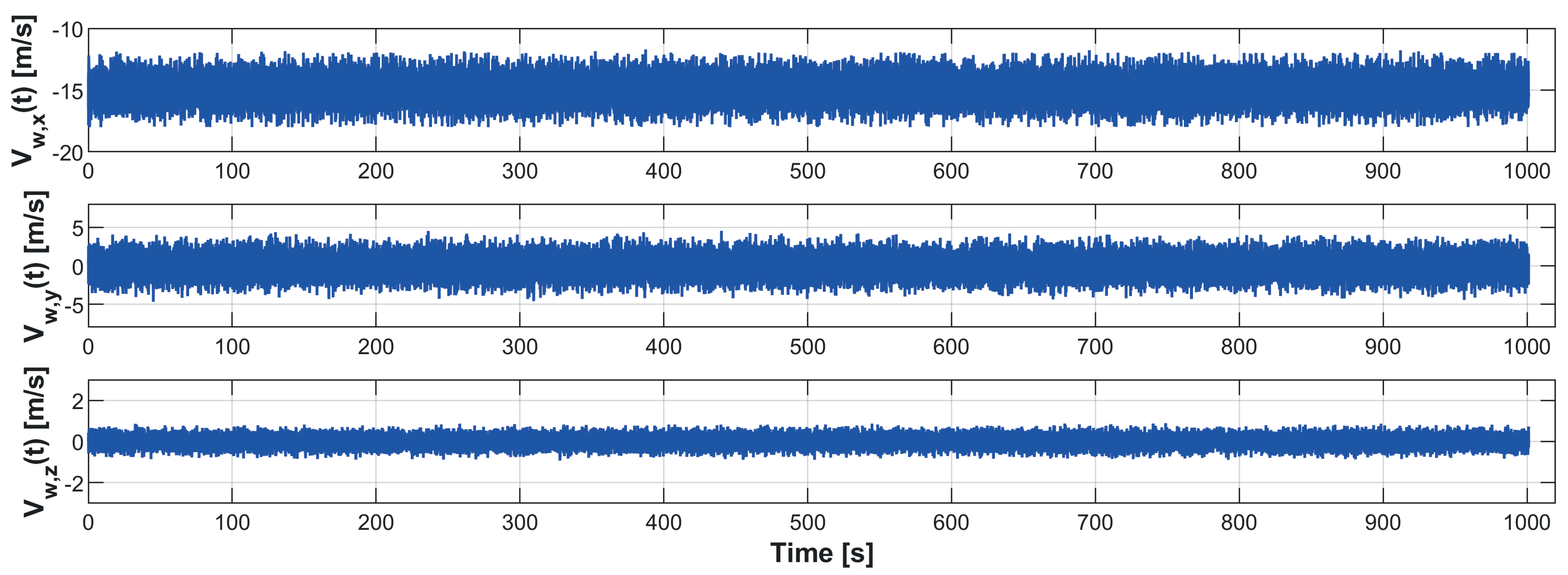
The governing equations of the UAV’s motion were given by a typical flight mechanics model and appropriate thrust and fuel consumption equations [41,42,43,44], although several fundamental aspects were adapted to this case, such as the time variation in the mass, mass center, and inertia matrix, as well as a non-null atmosphere motion. The UAV model is fully detailed in [45]. A simplified normally distributed wind model was supposed based on [46,47,48], and average wind velocity and direction values in the operation area were employed (see Table A1 and Equations (A1) and (A2)) [49,50]. The atmospheric parameters were provided by the International Standard Atmosphere (ISA) [43,51,52].
2.1. Dynamic Trajectory
In order to accomplish the mission, a 3D representation of the complete environment had to be conducted, in which restrictions were introduced. The flying system had to ensure the construction of a realistic dynamic trajectory for the UAV while avoiding demanding turning rates and excessive accelerations or decelerations as much as possible, since the control and guidance systems were not able to track the reference. To prove the performance of the flying system, a hypothetical military mission is proposed.
2.1.1. Three-Dimensional Space Creation
The whole space in the plane was defined by the initial and final points. Regarding the z coordinates, the range of values was determined by the sea level altitude and a maximum reference altitude.
Each pair of latitude and longitude coordinates were translated into a couple by means of the great circle distance concept, which defines the shortest length between two points across the globe.
2.1.2. Obstacles
In a real military mission, static and dynamic obstacles can be found; however, only static ones were considered in this case, since no enemy patrols were expected to be encountered. The following elements were used to define the environment of action:
- 1.
- Danger area: Zone in which the aircraft was not allowed to enter, generated as a cylinder from the sea level altitude to the maximum altitude.
- 2.
- Radar area: Similarly to the danger area, the radar area approximated the scope of an enemy radar. It was defined as a cylinder, with its bottom altitude determined by the minimum altitude at which the UAV could be detected.
- 3.
- Dropping slope: This is not a real obstacle, but instead was employed to ensure a correct descent of the aircraft when it approached the objective, generated as an inverted cone whose vertex was .
- 4.
- Ground elevation: Through mapping based on a digital elevation model (DEM) [53] called the National Elevation Dataset (NED) [54], provided by the United States Geological Survey [55], the mountains of the environment were properly defined. The resolution provided by these data was between 30 and 60 m. First, a planar mesh defined by the latitude and longitude coordinates was created in Keyhole Markup Language (KML) [56]; then, it was converted into GPS exchange format (GPX) [57,58], and the elevation data were introduced.
2.1.3. Mission Specifications
The F-86 Sabre, which began acting as a flight bomber during the Korean War (1950–1953) [59,60], was hypothetically modernized in order to enhance its military functionality. Nevertheless, this new technology has not yet been tested in this aircraft in autonomous bombing operations; therefore, the United States Air Force (USAF) has decided to conduct a mock blitz in the Center Eastern region of Alaska. The mission will consist of bombarding an uninhabited area close to the border with Canada at a minimum vertical distance of 200 m, starting from the Eielson Air Force Base at an altitude of 1200 m. The Sabre will have to face a radar with a minimum detection altitude of 900 m and two danger areas, with a maximum dropping slope of 2.
Figure 2 represents a sketch of the operation environment from Google Earth and the required restrictions, which are shown in the 3D space.
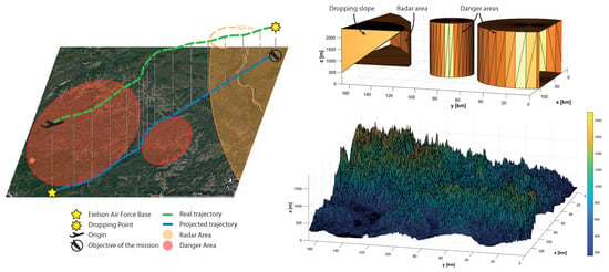
Figure 2.
Initial and final points of the mission and restriction areas (left). Obstacles of the danger and radar areas and the dropping slope (top right), as well as the ground elevation (bottom right).
3. Dynamic Trajectory Planning
3.1. Adaptive Cell Decomposition
A typical 3D ACD algorithm attempts to conduct a discretization of the environment in a tree data structure known as Octree. The algorithm verifies a possible collision of each rectangloid with the obstacles at each decomposition level; afterwards, independently of whether a potential collision is identified, all subspaces are divided into eight new children. When the final decomposition level is attained, all children identified as potentially colliding with obstacles are discarded, taking only the collision-free rectangloids. Furthermore, in this case, regardless of whether a subspace is fully included in an obstacle, that subspace is rejected and not divided into new ones at the current decomposition level.
Algorithm 1 shows the pseudo-code utilized in the discretization process. Once the decomposition level (n), obstacles, and initial space are defined, the decomposition starts from the first level to the nth level. At each step, all subspaces of the same level are analyzed (from to p), provided that they are not fully included in any obstacle (complete collision). The term refers to a 3D matrix that contains all subspaces generated by the algorithm, so that each rectangloid is represented by a position and a group of eight vertices. Then, the vertices of the children are calculated by the function and the collision object of each rectangloid is generated by the function. When the final decomposition is completed, the selection of collision-free rectangloids is accomplished, obtaining a list with their positions in the matrix.
| Algorithm 1 Adaptive cell decomposition (ACD) |
|
This list, together with the vertices of the collision-free subspaces, was employed in the recursive rewarding adaptive cell decomposition (RRACD) algorithm to determine the next possible waypoint on the route.
This methodology is not the most efficient in the computational sense, as it would be more adequate to divide only rectangloids with verified collisions, as is done by the modified ACD algorithm in [14]. However, the basic ACD methodology was preferred, since it facilitates waypoint selection by offering a wider range of possibilities.
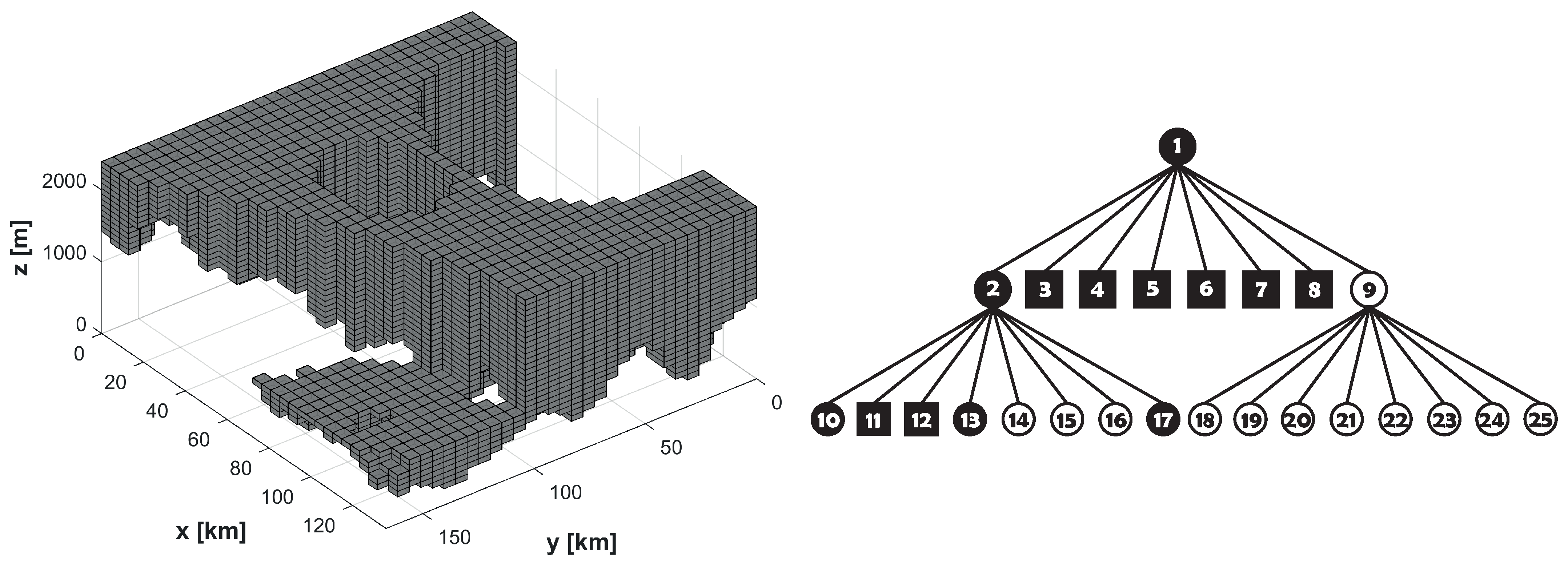
In Figure 3, an example of the application of the ACD algorithm to the complete space of study is shown. Moreover, the tree scheme used for the Octree decomposition is represented: The verified and non-verified collisions (black and white circles, respectively) were divided into eight new rectangloids, while the inclusions in the obstacles (black squares) were discarded. This scheme is based on [61].
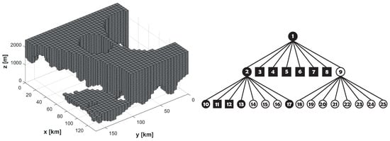
Figure 3.
Total free 3D space calculated using the adaptive cell decomposition (ACD) algorithm with a decomposition level of (left) and a tree scheme of a hypothetical Octree block (right).
Furthermore, to diminish the danger of extreme closeness to the terrain, a security distance equivalent to three times the aircraft’s wingspan was introduced in the elevations of the ground collision mesh object, allowing for a more secure flight.
3.2. Recursive Rewarding Adaptive Cell Decomposition Algorithm
An approach to a node-based algorithm was created herein, although the centers of the rectangloids were used instead of edges and vertices, and the optimization parameters comprised the distance and the course and flight path angles. The RRACD algorithm defines a final path by means of the initial subspaces, so that a starting decomposition of the complete environment is made, assigning to all rectangloids a collision-free grade. The initial level selected for this case was (), giving, as a result, a number of starting rectangloids of .
Afterward, beginning at the initial point () as a free subspace (), the algorithm searches for neighboring rectangloids () from the initial decomposition and divides them into new ones () by utilizing the ACD code at a level of , which is equal to 3 for this operation. It is important to mention that the complete decomposition is limited, since the final rectangloid dimensions must be greater than the planar accuracy of the ground elevation mesh. The most adequate neighboring option is found by the sum of and , two rewarding functions that measure the cost of selecting a future destination. This procedure is repeated until the final point () is attained.
is obtained from the path analysis of to () and from to (). Each one is defined by a set of partial functions in combination with a Gaussian function and the weight parameters (for ) and (for ).
The set is a group of partial functions that involve 3D flying characteristics. In the algorithm, a total of functions are defined (position n) and further divided into types 1 and 2 (position m) in relation to the subpaths and , respectively. Type 1 functions take into account previous course and flight path angles to measure their variations, while type 2 functions only consider the angles of the subpath.
- 1.
- Distance: Given by the expressions below, where is the Euclidean distance between the chosen subspaces and , and is the straight line between and .
- 2.
- Flight path angle: Where is the flight path angle of the previous branch of the path and is one of the vectors given by . The functions must provide a value between and 1, so that in cases in which , the output will be 1.
- 3.
- Course angle: is the course angle of the previous branch of the path and is one of the vectors given by . As before, when , the output in the code will be 1.
Regarding the Gaussian function utilized to analyze the reward in executing a possible action, it is defined by the expression (7), in which the transition cost values () have been normalized within the boundaries .
It is important to note that the higher the effort , the smaller the reward , and vice versa. All of these rewards are collected in the vector :
Finally, , the priority parameters (), and a new parameter are employed to build the a final rewarding function , which is composed of and . The neighbor with the greatest reward is selected as the next waypoint on the route. The reward of selecting a subspace is given by the following expressions:
The parameter is a variable reward value that is assigned to the neighbors that are considered as very problematic or extremely necessary given the aircraft position and the obstacle locations. For instance, before entering into the radar area, the aircraft must decrease its altitude significantly to cross it successfully, so that only the neighbors that are located in a lower position at each step will be scored with a positive .
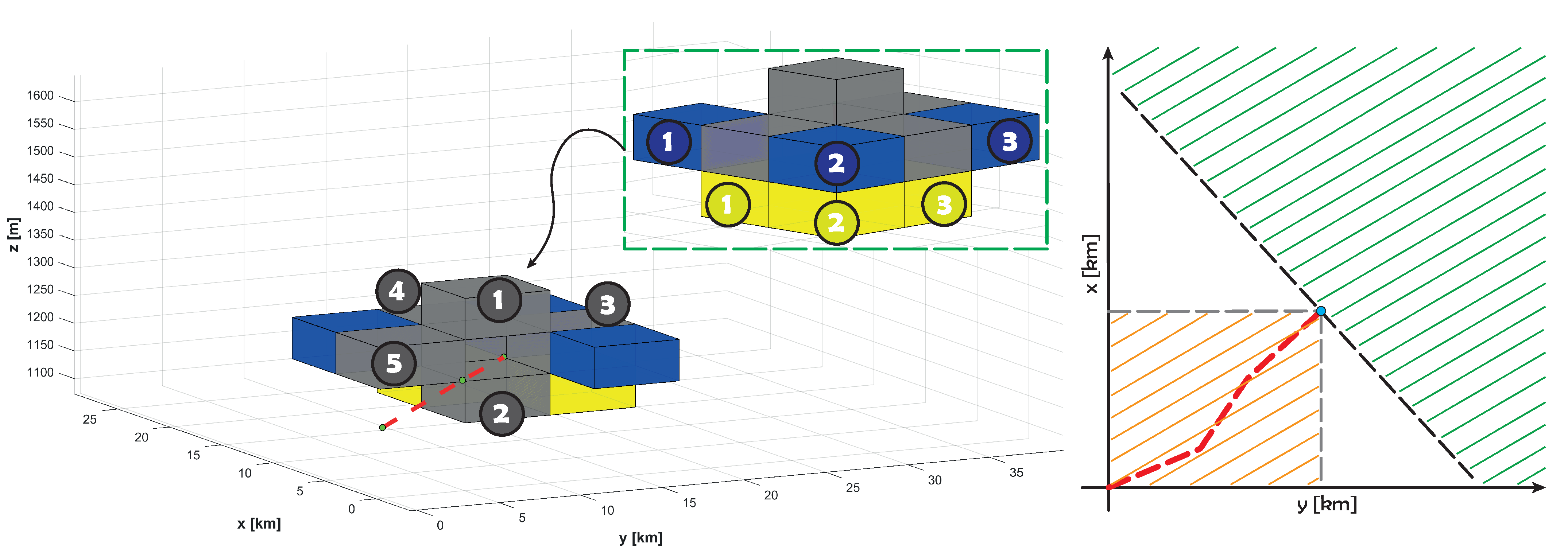
Regarding the neighborhood choice, the block subspaces located on the top, bottom, sides, and in front (gray) of the subspace are evaluated as neighbors (see Figure 4). Furthermore, three diagonal rectangloids (blue) are permanently available neighbors for improving the algorithm’s capabilities in the path-building process, while the other three on the bottom front, diagonal, and right sides (yellow) are introduced when the aircraft is close to the radar’s perimeter in order to facilitate the descent. If the UAV has already been to one of these possible subspaces, it is automatically eliminated from the list of destinations. Once the neighborhood has been obtained, the ACD algorithm is applied at each subspace, and afterward, the centers of all new rectangloids for which the rewarding function is used are calculated so as to choose the next most appropriate destination.
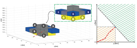
Figure 4.
Examples of the possible neighbor subspaces at a point in the path (left); the available area in the plane in green and the fully forbidden zone in orange (right).
In addition, dynamic restrictions are applied after all centers have been obtained. The centers that suppose a change in the course angle greater than 90 or imply the entrance of the UAV into a fully forbidden zone (see Figure 4) are discarded. Moreover, if the selection of a center entails the UAV navigating a trajectory with a flight path angle , this center is also rejected.
In Algorithm 2, the RRACD process is shown. First, the initial and local decomposition levels are defined, together with the rest of the variables. Then, the subspaces that have already been visited are discarded and the neighborhood is calculated. The ACD code is applied to each rectangloid and the available centers are calculated by the function ; in the case that there are no centers, a new process with a higher level of decomposition is performed. The rewards of the centers are obtained, selecting the point with the greatest reward. is calculated every time, so that if the last waypoint is fairly close to , the algorithm takes it directly.
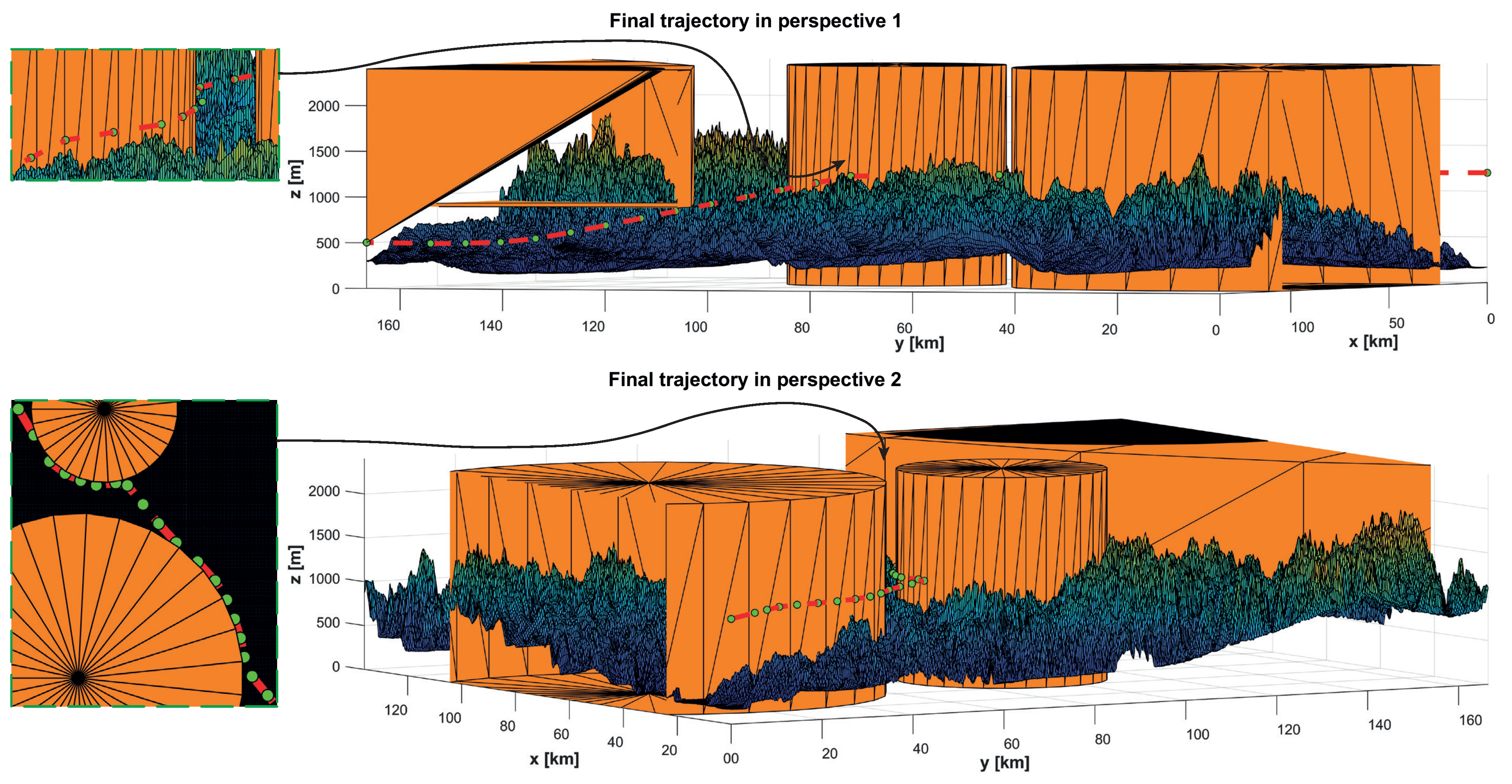
The final reference trajectory, which is shown in Figure 5, offers acceptable flight conditions and avoids all imposed obstacles. However, this is not the best possible solution, and different combinations of weighting parameters should be selected to enhance the results.
| Algorithm 2 Recursive rewarding adaptive cell decomposition (RRACD) |
|
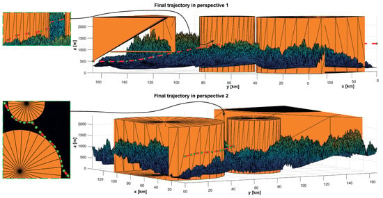
Figure 5.
Final trajectory obtained by means of the recursive rewarding adaptive cell decomposition (RRACD) algorithm.
3.3. Trajectory Smoothing
Although the path obtained by the RRACD algorithm is appropriate for UAV guidance, sudden changes in direction when passing a waypoint are impossible for an aircraft to achieve, which could thus provoke excessive maneuvers by the UAV in the guidance process; therefore, the radii of gyration are applied to obtain a smooth trajectory, which is easier to track than the previous one. However, this smooth path could collide with obstacles; hence, the possibility of collisions is analyzed to ensure that this does not happen, and if it does occur, the radii of gyration are diminished in the conflict regions. Thus, the smooth 3D path-planning algorithm finds the optimal trajectory in terms of low angle variation rates and obstacle avoidance based on some concepts from [62]. Moreover, a velocity profile is designed by the algorithm.
The algorithm is applied to each non-aligned group of three waypoints. In Figure 6, an example of the application of the radii of gyration is represented, in which points and are the tangential points among the arc and both lines, vectors , , , and are the tools utilized to define points and , as well the arc center (O), and R is the radius. The directions of vectors and are the result of the following vectorial product: .
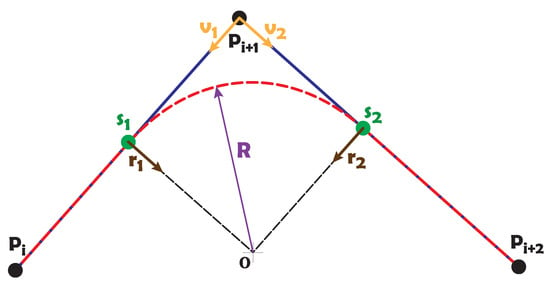
Figure 6.
Radii of gyration: reference trajectory (blue), waypoints (P), smooth path (red), radius (R), center (O), and tangential points (s).
The generation of the final smooth trajectory is made by means of two steps at each iteration: first, the path and velocity profile using Algorithm 3, and second, analysis of the errors in the trajectory building and collision of the new path with the obstacles, which are conducted using Algorithm 4.
| Algorithm 3 Smooth 3D path simple design (S-3D-PSD) |
|
| Algorithm 4 Smooth 3D path planning (S-3D-PP) |
|
Regarding Algorithm 3, the first step consists of initializing the required variables: The path, yaw, and flight path angles obtained from the RRACD code; the maximum, minimum, and initial speeds in the velocity profile; the maximum positive velocity variation per meter (); the precision of the trajectory building (); the minimum load factor used at each curve (); the maximum allowed load factor () [40]; the vector . The vector contains the gradient of the load factor with respect to the yaw angle change (), so that when a change in takes place, an additional load factor is applied. Therefore, the formula for the load factor in the case of i is given by the expression:
Afterward, the code examines the complete reference path by applying the radii of gyration when any change in the course or flight path angles occurs, which can be approximated by [43]. Vectors and and their angle are obtained; then, the load factor is obtained from the expression (12) to calculate the radii of gyration, which are restricted to the radius corresponding to . After that, the distance and the vectors and are calculated, from which points and and the center O are found.
Finally, the points from to , which contain the arc, are obtained by the function. These points also include all of the velocities as a fourth element, except the 3D coordinates. The variable can be 0 or 1 and determines whether a radius of gyration has been applied in the previous group of waypoints in order for the path to be built properly. In the case of an aligned group of waypoints, the function generates a straight line.
Once a first dynamic trajectory is generated, Algorithm 4 attempts to find possible errors in the construction due to overlapping arcs and studies whether the new trajectory collides or not. At the beginning, the load factors are set at low values to create big radii of gyration in order for the algorithm to be able to find the optimal solution by means of optimizing the vector . Therefore, the code analyzes which waypoints are problematic and adds to their respective parameters and values, increasing the load factor in the points that have excessive radii of gyration (these positions are defined by the vector ) and trying to prevent the arcs from overlapping or colliding with obstacles. Every time a building error or collision is found, the whole code generates a new trajectory with the improved vector; hence, only when the new path is perfectly well defined can the algorithm end and the solution be obtained.
Finally, a new trajectory course and its time derivative and flight path angles are calculated with the function.
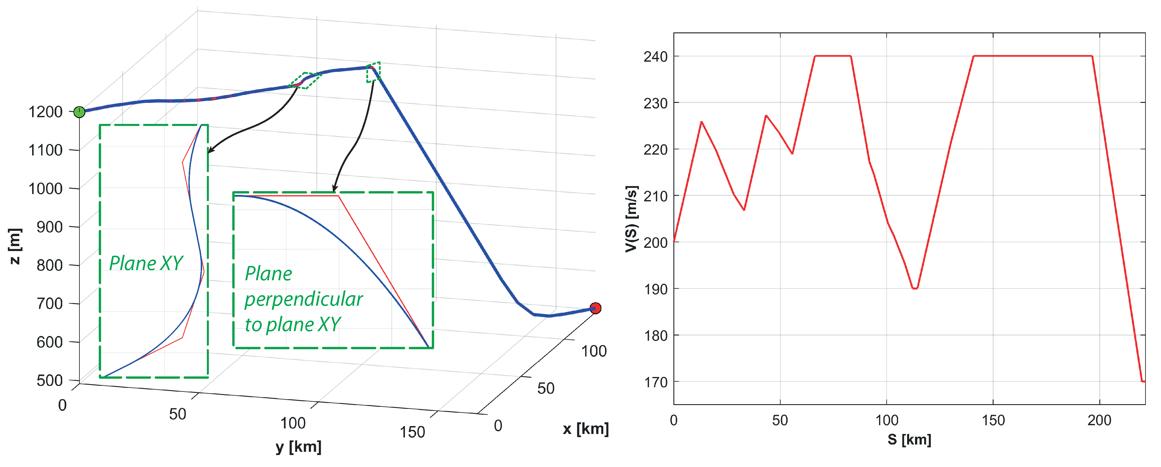
In Figure 7, the final results of the algorithms are shown. The parameters utilized in this case are:
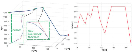
Figure 7.
Final trajectory obtained by the 3D smooth path-planning algorithm (left, original in red and final in blue) and the velocity profile as a function of the curvilinear distance S (right).
The velocity profile is created with the purpose of reducing the speed during curves and descents, while it is increased for straight lines in order to minimize the flight time and to make the dynamic trajectory easier to follow. In addition, the desired velocity of a bomb dropping at m/s is selected to accurately impact the objective; hence, the UAV must progressively diminish its speed when it is close to said objective.
4. Guidance Law
A nonlinear guidance law induces an acceleration in an aircraft to incorporate it into the reference trajectory. In this case, the acceleration is only in the horizontal plane, seeing that the control is conducted on the altitude state variable and not over the flight path angle.
This force is applied perpendicularly to the velocity vector () according to the expression (14). N is a proportional gain that must be adjusted to achieve greater or lower accelerations depending on the case because an excessive value can produce an unstable flight with many oscillations, while a low value generates poor adaptive guidance when the UAV faces changes in the reference. is the relative position vector and is the angle between and .
The desired trajectory of interception is circular, so that the length of is defined by the radius R of such a circular motion. Both the target in the reference path and the instantaneous aircraft location are points of this circumference. In Figure 8, this process can be observed.

Figure 8.
Conceptual guidance system (left) and nonlinear guidance law (right) schemes.
In addition, in Figure 8, a simplification of the GNC system scheme is shown. The code composed of Algorithms 1–4 sends position and velocity data to the guidance system. The guidance law creates an utter reference in altitude, attitude (roll and yaw angles only), and velocity based on the navigation information. These new references are analyzed by the control system, which generates the required control action signals. Note that, as mentioned in Section 1.2, the navigation problem has been simplified by assuming that the state vector of the aircraft is completely known.
The attitude control cannot accept accelerations; consequently, the horizontal force is translated into a desired course angle (), from which the required yaw angle () that the aircraft must achieve is obtained. At each sampling time (), a command of the course angle change () is given. The expression of this angle change is as follows:
The velocity and bank angle () are assumed as constants and the flight path angle () as null, and a symmetrical flight is also supposed, resulting in the bank and roll angles () being equal [32]. These hypotheses, defined by the expressions (16) of uniform circular motion in the horizontal plane, are no longer true if the sideslip and flight path angles are very different from zero, but this is the best approximation for achieving a set of equations that allows one to obtain a manageable solution of the reference roll angle.
Hence, the new horizontal acceleration is . These conditions are translated into expressions for the load factor and the roll angle of the aircraft, defined by the following equations:
In addition, the load factor must be between boundaries in order to guarantee stall avoidance and exceeding the structural limits; therefore, the load factor value must ensure that:
Once the fundamentals of this guidance law are detailed, Algorithm 5 is implemented, which attempts to find the desired target point at each time step and defines the reference in the velocity, altitude, and roll and yaw angles.
| Algorithm 5 Nonlinear guidance law |
|
First, the current flight parameters are defined, together with the aircraft parameters (, m, and ) and the threshold, which is the length that specifies whether the simulation stops when the distance between the aircraft and the final destination is lower. is provided by the dynamic trajectory-planning process and includes reference 3D coordinates and velocities.
The radius R is calculated from the velocity, taking greater values for high velocities and lower values if the speed is minimum. Afterward, the coordinates of the intersection point between the circle, whose radius is R and whose center is the aircraft position, and the trajectory are obtained. There are two intersections, so the one with a higher index is chosen. Second, repeating the same procedure but without the radius, the closest point of the reference path to the aircraft position is selected to specify the altitude and velocity to be tracked.
Afterward, the relative position and velocity vectors in the plane are obtained, so that the changes in the course angle (), the load factor (n), and the reference roll angle () can be calculated by means of the previously explained equations. Then, the reference yaw angle is achieved by means of the rotation matrix , which translates the velocity in body axes into plane motion with the aircraft’s direction, as well as the course angle. Finally, the distance from the aircraft to the final destination is analyzed, so that if it is lower than the threshold, the simulation ends.
5. Control Strategies
In order to develop a control system, the mathematical model must be linearized beforehand with respect to an equilibrium point. The equilibrium conditions correspond to the trimmed point of the aircraft in a vertical planar motion characterized by the given velocity and altitude values. In this case, m/s and m are utilized, which are the mean values of the dynamic trajectory obtained in the previous chapter.
If the system of equations obtained from the linearization process is rearranged, a linearized state–space model can be achieved, given by the expression (20), in which represents the state variables, the control variables, and d the modeled perturbations. A is the system matrix and B is the control matrix, while is the disturbance matrix. All variables are given in increments with respect to their corresponding equilibrium position values. Attending to the Equations (A3) and (A4) of these matrices, all variables are interrelated; hence, the longitudinal and lateral direction motions are coupled.
The chosen state variables are the body velocities (u, v, and w) and the angular body velocities (p, q, and r), the Euler angles (, , and ), the altitude (z), and the total body velocity (V). The control variables are the throttle lever activation () and elevator (), the ailerons (), and the rudder deflections (). To facilitate the control system design, the perturbation variables are also added to the control variables, i.e., the wind velocities in the fixed axes (, , and ) and the drag compressibility coefficient (), since they are zero when the Mach number is below the divergence number () [43]. The implemented linearized state–space model is as follows:
In addition, regarding the sample time, it must fulfill the Nyquist theorem [63], in which this parameter must be less than the settling time of the system to allow an acceptable control. In this case, the settling time of the system is related to the sixth eigenvalue of the system matrix. The selected sample time is s, so that it satisfies the requirement:
5.1. Linear Quadratic Regulator
An LQR is an optimal control technique that provides the best possible performance with respect to some given performance index. The LQR design problem involves the design of a state feedback controller K such that the objective function is minimized [64]. In this technique, a feedback gain matrix is designed that minimizes the objective function in order to achieve some compromise between the use of control effort, the magnitude, and the speed of response that guarantee a stable system. The function proposed in this work is the well-known cost index described in (25) [27]; although the weighting matrix is typically considered null, the cost function becomes a quadratic one.
Q and R are the weighting matrices for the state and control signals, respectively, and are defined by the designer such that and . The higher the weighting value, the lower the state or control action associated with that value. Regarding the calculation of the matrix K, it is obtained from the Riccati equation [28], where S is the Riccati solution to the equation:
Since the longitudinal and lateral direction motions are coupled during flight, it is necessary to separate them in order to develop an appropriate LQR controller. Hence, four different subcontrollers are created so as to fulfill the requirements, so that four feedback gains can be obtained: , related to the altitude; , related to the speed; and , related to the tracking of the roll and yaw angles. The reference following and is complex; thus, a unique feedback gain does not provide an adequate response, resulting in a requirement to use two feedback gains in a cascade configuration.
In this way, and assign the required elevator deflection and throttle lever action to follow the reference in altitude and velocity from the guidance algorithm, respectively. In relation to the roll and yaw angles, creates a reference in angular velocities p and r on the basis of the error in these angles with respect to the reference; however, this error is not integrated because a very aggressive and fast action is demanded. Afterward, the feedback gain is applied to this error. The state and control variables and cost functions corresponding to each feedback gain matrix are given by the following expression:
In order to build these matrices, amplified subsystem matrices must be created. These matrices include the errors () in the variables to be reduced. Hence, the state variable vectors comprise an amplified vector, which also contains the variables of error. In addition, matrix Q presents in its diagonal the weighting factor for each variable of the new amplified state vector. As can be seen in Equation (A5), in matrix Q, the elements corresponding to the error variables are much more important for prioritizing the tracking error and for diminishing it as much as possible. Moreover, the elements from matrix R are considerable in size, since only necessary control actions should be used instead of excessive ones. However, these values are limited because they could be unreasonable as a result of poor control actions; therefore, there is an equilibrium between the Q and R matrices that provides balanced control responses.
5.2. Model Predictive Control
MPC is a strategy that uses an explicit model of the process where, at each sampling time and with the current information of the process variables, predictions of future process behavior along a horizon are managed. Such predictions are incorporated into a cost index to solve an open-loop optimal control problem (OCP) that is subject to constraints, which results in the sequence of future optimal controls.
Consider the discrete linear system (31), where variables and represent the state vectors and system inputs, respectively, at the instant ; A is the state matrix and B is the system input matrix
For every instant k, based on (31) and with the availability of the current state of the plant , predictions are made for the states and inputs along a prediction horizon N, . These predictions are included in the quadratic cost index (32), which is subsequently minimized at the OCP (33):
where the current state is known; thus, ; matrices Q, R, and are weighting matrices that penalize the first N predicted, predicted inputs, and terminal state, respectively. The matrices Q and R (equivalent to matrices Q and R in LQR controllers) are defined by the designer such that and , and is obtained from a quadratic stability analysis [65,66,67]. Notice that the subscript indicates the predicted value of the variable for the instant based on the information available at time k.
In each control period, the problem stated in (33) is solved, obtaining the vector of optimal decision variables , which drives the system states to a desired operating point [68] or as a regulator towards the origin. Next, applying the receding horizon strategy, only the first element from the control sequence is used, so that OCP (33) is performed again at time .
The cost function (32) obeys the dual-mode prediction paradigm [66,69,70], which ensures stability for an appropriate (or long enough) horizon N, incorporating a terminal cost that penalizes the terminal state . Another condition that is also used to ensure closed-loop stability is to complement the dual mode by adding the terminal constraint [69,71] to the OCP (33). The purpose of this is to force the terminal state and the following states to remain within a safe zone or terminal set [65,72,73].
The OCP (33) is stated as subject to constraints (34)–(38). Notice that constraint (34) indicates that the predicted state is computed recursively using the state and inputs from the previous state , where . Linear inequalities (35) and (36) are constraints for the predicted states and input trajectories, respectively, where matrices H and D and vectors h and d represent the constraint limits.
Given the quadratic and convex nature of (33), the linear model (31), and the types of constraints (35) and (36), a finite-horizon OCP stated as in (33) can be solved at each control period. This OCP is a quadratic programming problem (QP) with a global optimum whose solution results in the optimal control vector.
In addition to the theoretical formulation, Figure 9 intuitively shows how the MPC works.
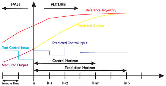
Figure 9.
Model predictive control (MPC) future prediction scheme.
The control horizon must always be lower than the prediction horizon. Furthermore, an adequate combination of sample time and control and prediction horizons should be made, since a low control horizon or a high sample time can lead to poor control actions and vice versa, while low prediction horizon values could demand excessive or even impossible control actions.
The prediction and control horizon parameters are set to 100 and 10, respectively. Therefore, at each iteration, the controller calculates the performance of the system for a total of s by means of applying control actions until time s, selecting the best options among all of the calculations.
Additionally, the physical constraints shown in [40] are introduced into the MPC following the OCP structure. This is because it is not necessary to include a signal filter after the control block, as is done in the LQR controller.
The controller responses are determined by the weighting matrices Q and R applied to the state variables and control variables. Tracking is only performed for the altitude, velocity, and roll and yaw angles.
As shown in Equation (A6), some variables are specifically high in the weighting matrices Q and R; the pitch angle, angular velocity q, and elevator deflection are prioritized to avoid excessive motion in the vertical plane and altitude errors.
6. Results
6.1. Complete Response
The flight simulations utilizing both controllers, i.e., LQR and MPC, were performed under variable mass and wind conditions, as explained in Section 2. The wind velocities in each axis obtained during the simulations are shown in Figure A1. The compressibility effects are not given, since the divergence Mach number was not exceeded.
The code developed to perform all the simulations is available on Matlab Central [74], including the path-planning algorithms, control parameter definitions, and Simulink files, in which the controllers and guidance law that were employed in simulations are implemented.
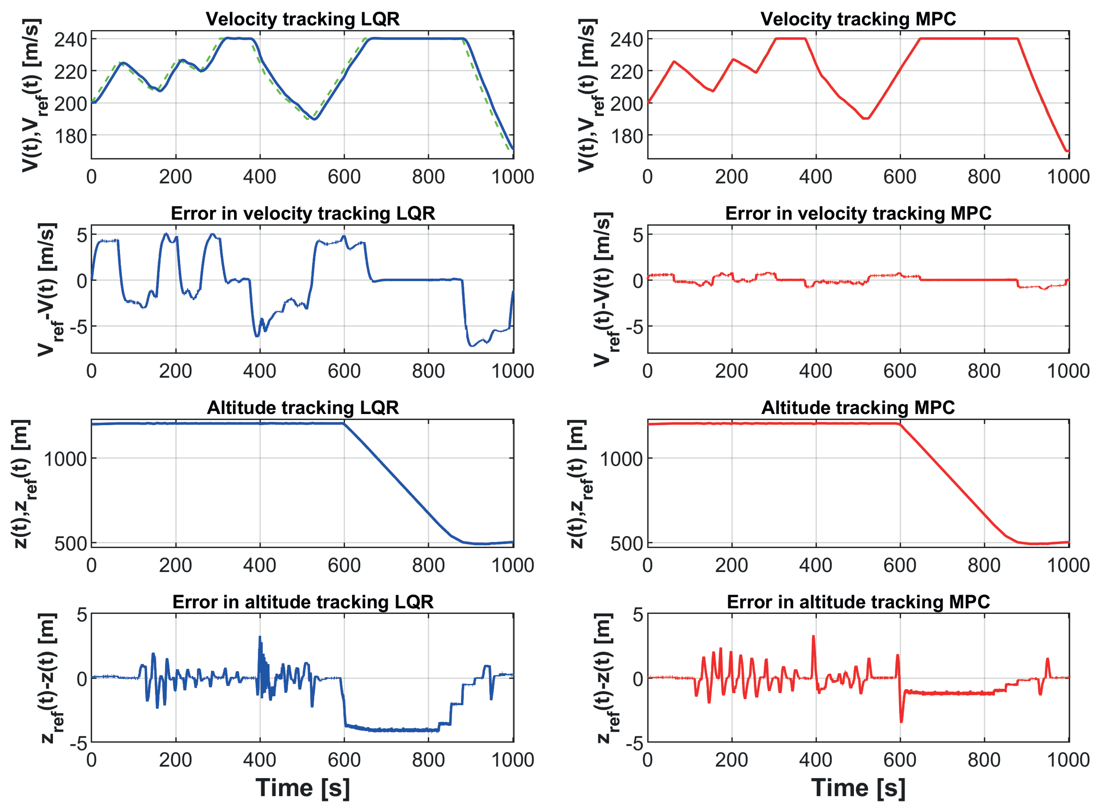
In Figure 10, the velocity and altitude magnitudes are shown, together with their respective reference values specified by the dynamic trajectory. The MPC case clearly provided a more satisfactory response in velocity tracking, while the reference altitude was followed similarly in both cases. Nevertheless, the LQR controller showed several problems during curves and descents, since the velocities and altitudes presented considerable errors, while the MPC controller achieved a more satisfactory performance.
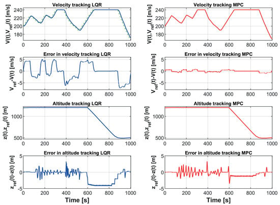
Figure 10.
Reference tracking of velocity and altitude: linear quadratic regulator (LQR) (blue), MPC (red), and the reference for each case (discontinuous green).
When great differences with respect to the equilibrium point were given in the flight path and roll angle (in the state–space model, and were considered null due to the trimmed point conditions), such as in intense descents or curves, the longitudinal and lateral direction motions were coupled to a considerable extent, which provoked acute errors in the reference tracking, since the LQR and linear time-invariant MPC controllers worked continuously with the same plant model. In this case, both of the controllers’ performance during curves showed appropriate robustness, although the MPC controller more adequately tracked the reference velocity.
Generally, an MPC controller creates more adequate control actions than an LQR controller due to its future prediction capabilities; however, both controllers really depend on the selection of the weighting parameters. In the case of the MPC controller, their suitable selection, which restricts the pitching motion and assigns a high priority to altitude and velocity tracking, provided satisfactory results during the whole simulation. Regarding the LQR case, the parameters of the Q and R matrices and the structure of this controller were selected appropriately. The special configuration on the part of the LQR controller corresponding to the roll and yaw angles led to stronger capabilities of tracking the trajectory.
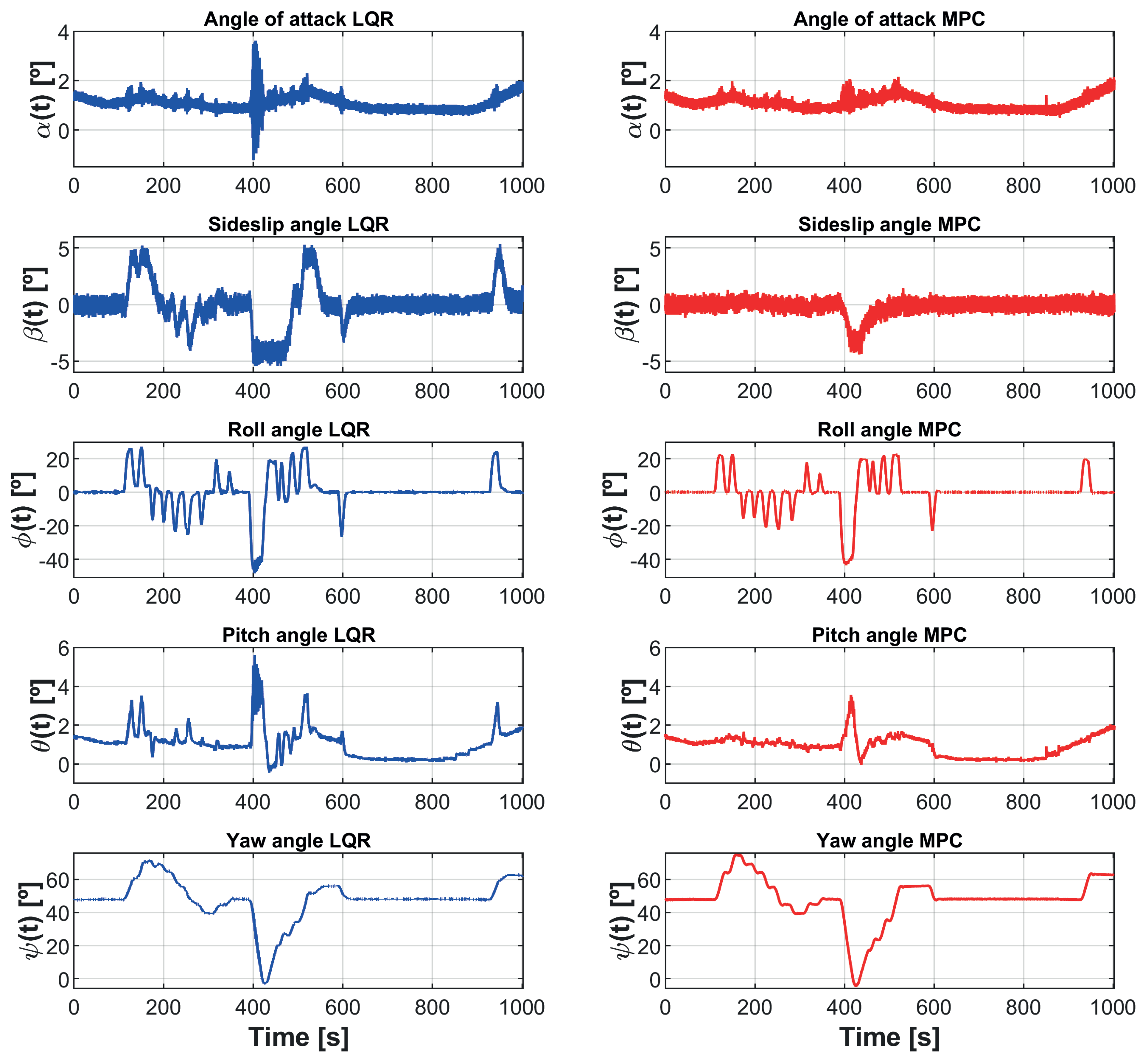
In Figure 11, several of the principal flight parameters are shown: the angle of attack, sideslip angle, and Euler angles. As can be appreciated, the fluctuations are fairly intense in all variables due to the wind, although they are especially relevant in the sideslip angle.
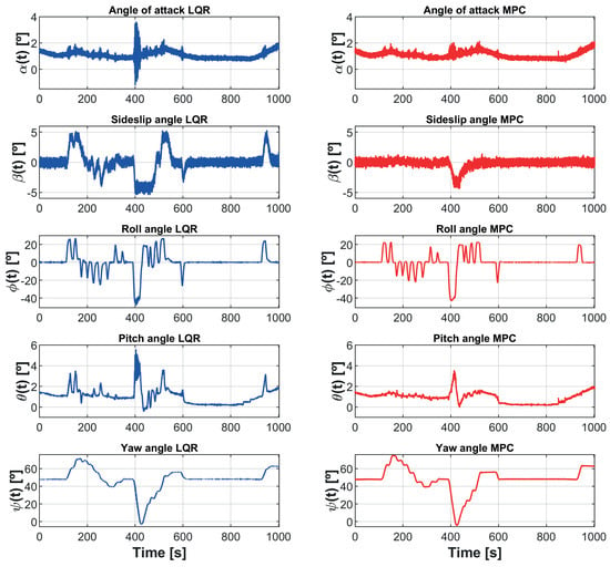
Figure 11.
Principal flight parameters by LQR (blue) and MPC (red): the angle of attack (), sideslip angle (), and Euler angles ().
The angle of attack presented realistic values in almost all of the trajectory, but in some points, it entered into the negative area due to aggressive control actions, which is correlated to the error in altitude tracking shown in Figure 10. These negative values enlarged the probability of stalling in the real behavior of the UAV, so that the LQR controller could produce several failures in this sense, such as, for example, at a time of s.
With regard to the sideslip angle, in no cases was it null because the wind velocity restricts the yaw and course angle from coinciding in straight lines. Also, this parameter showed very well the regions where the turns occurred. Concerning to the notable curves, if they are made in the clockwise direction, the sideslip should be mainly positive; on the contrary, counterclockwise curves provoke negative sideslip angles. Therefore, the LQR results present a more clear development of the aircraft rotation for proceeding with curves properly, while the MPC results represent a more erratic behavior.
Considering to the pitch angle, the motion was more aggressive in the LQR case because the elevator control action was not as anticipatory as that of the MPC controller, which demonstrated excessive oscillations in the angle of attack and altitude tracking errors. Last but not least, the roll and yaw angles were very similar in both cases; however, they presented lower fluctuations and overshoots in the MPC case. Therefore, the guidance law acted slightly more ineffectively for the LQR controller, or the controller was not robust enough in the lateral direction motion.
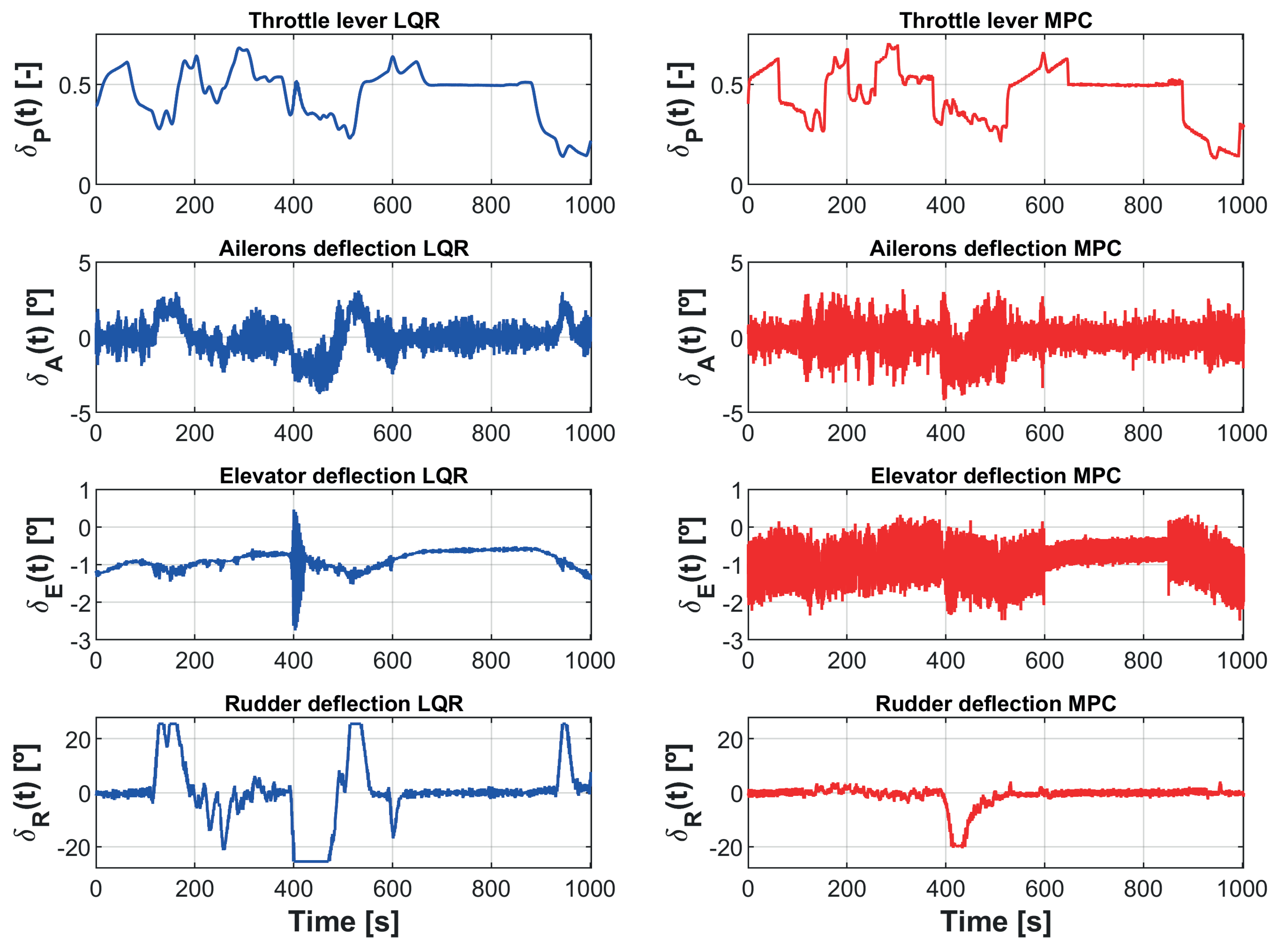
The control action signals are given in Figure 12. More intense fluctuations in the control actions were obtained in the MPC results, which confirms the previous results, in which the flight parameters oscillated less. The amplitude of the oscillations in the control signals of the rudder was primarily higher in curves in the LQR case, demonstrating a more aggressive control for facing perturbations and adequately tracking the reference path. In relation to the ailerons and elevator deflections, regarding the former, their fluctuations were comparable in both cases; meanwhile, regarding the latter, their oscillations were chiefly more intense in the MPC case, although their average value was very close to that of the LQR controller, owing to the improvement of the stability of the aircraft by the greater robustness of this controller.
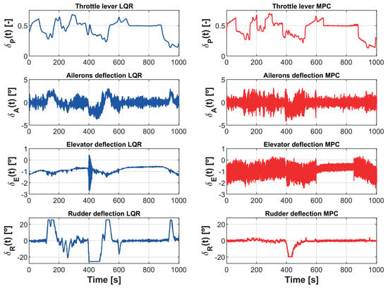
Figure 12.
Control actions by the LQR (blue) and MPC (red) controllers: the throttle lever () and elevator (), ailerons (), and rudder () deflections.
The error in altitude can be explained by the non-coordinated control actions of the elevator because the controllers utilized it without taking into account that it also interferes in the lateral direction motion because of the linearization process with respect to the trimmed point.
In addition, the mean value of the oscillations in the rudder along the straight path was not zero. This was due to the fact that the course angle was not exactly the one specified by the guidance algorithm and the sideslip angle fluctuated with respect to an angle higher than zero (see Figure 11). This problem was less significant in the MPC case, which could be due to the well-coordinated control actions between the rudder and ailerons.
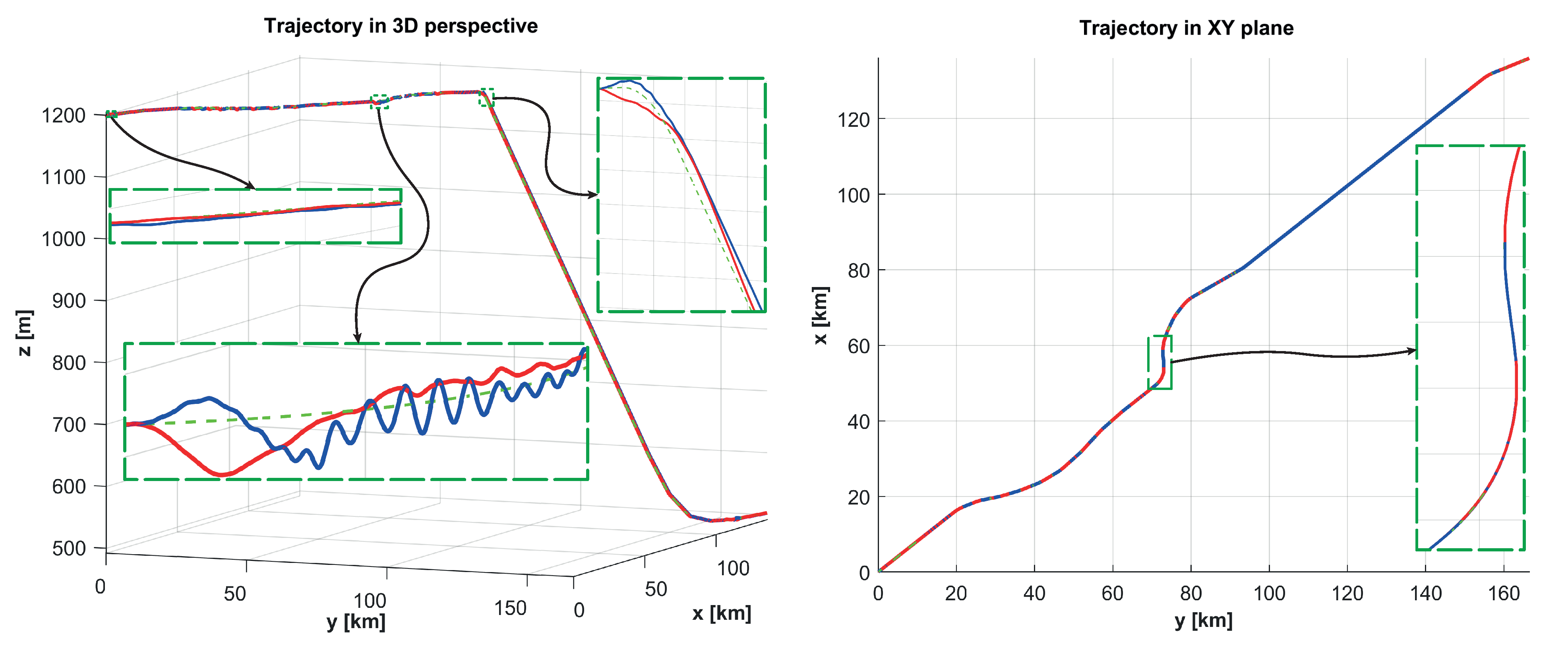
Finally, in Figure 13, the trajectories of both cases are shown. The errors in altitude were similar in the LQR and MPC cases, as can be seen in the figure. In relation to the tracking of the path in the plane, both controllers provided satisfactory results, since the deviation was minimum; nevertheless, if more intense curves were given, the LQR would accomplish a slightly more appropriate planar tracking due to its adequate coordination of the control signals, as shown by the sideslip angle results in Figure 11. However, the clear advantage of the MPC was in the velocity results, as can be observed in Figure 10.
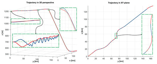
Figure 13.
Final trajectory from two perspectives; LQR (blue), MPC (red), and reference path (discontinuous green).
6.2. Analysis of the Impact, Time, and Fuel Mass Consumption
By means of a dropping point estimation algorithm [45], which calculates the best location of the trajectory to release the bombs and their deviations in the impact, based on a mathematical model of M117 bombs [43,75] (detailed in [45]), the deviations in the dropping point from the reference release coordinates and the error in the impact—defined by the expressions (39) and (39)—were calculated in the LQR and MPC cases. This mathematical model assumes no gyration of the bombs around their x-axis; hence, only the yaw and pitch angles can vary. Furthermore, the mean wind velocity and direction were considered in the calculation of the reference case, while the normalized data were utilized in the real results.
Figure 14 represents an example of the application of the dropping point estimation algorithm. The bomb trajectories were calculated from each waypoint. Afterward, the most adequate dropping coordinates were obtained by means of diminishing the deviations in the bombs’ impacts, which were determined through the collision on the ground. The terrain was modeled through a bilinear interpolation [76].

Figure 14.
Dropping point estimation applied at the reference case: possible options (red lines) from suboptimal dropping points (green dots) and most appropriate option (blue line) from optimal release point (blue dot).
As can be seen in Table 1, the MPC controller offered more adequate results, since the deviations in the dropping point and error in the impact were fairly low, while the LQR’s dropping point was a considerable distance from the reference one, which means that the impact could be particularly inaccurate in terms of the real behavior. This can be explained by the appropriate velocity tracking by the MPC controller, since the error in speed during the drop was greater in the LQR case.

Table 1.
Deviations in the release (from reference case) and in the impact of the bombs.
However, these deviations could materially vary due to the fact that the bomb-dropping results are fairly contingent upon the final part of the dynamic trajectory. However, the velocity tracking of the MPC controller is still bound to guarantee a more appropriate response.
In addition, the flight time and fuel consumption were compared in order to evaluate the performance during the mission, since the relevant differences in these magnitudes could determine a greater efficiency of one controller over the other in the net results and because these magnitudes also provide a bigger picture of flight autonomy.
The flight time was slightly smaller in the LQR case, while the fuel consumption was lower in the MPC case, as can be seen in Table 2, although the differences were not significant. Hence, both controllers would be equally useful for missions.

Table 2.
Simulation time and fuel consumption.
7. Conclusions and Future Works
A realistic simulation environment was implemented for the F-86 Sabre acting as a UAV based on a group of known algorithms to analyze which multivariable control method provides a more satisfactory performance. This system was able to fulfill all of the mission’s requirements according to Section 2.
The dynamic trajectory-planning algorithms, which are modified versions of those in [14,45,62], demonstrated a proper behavior in the creation of waypoints for trajectories that are perfectly trackable for the aircraft and allow one to avert 3D obstacles. Furthermore, the 3D smooth path-planning code facilitated the reference-following task of the controllers. The reasonable velocity profile and the unusual approach of the neighborhood finding turned out to be appropriate for the path due to the fact that both controllers were able to perform adequate reference tracking. However, an improvement in these elements, as well as in the rewarding function and the selection of the center of the rectangloids, will be key to making further progress in dynamic trajectory building in future designs. For instance, the rewarding function could consider new flight parameters in its calculations and the center selections could take their proximity to obstacles into account to make the route more secure.
The LQR and MPC controllers provided acceptable responses, since the aircraft did not enter prohibited areas in either case, and the aircraft’s limitations were respected; nevertheless, the trajectory obtained by the MPC method was more satisfactory in terms of airworthiness.
Regarding the guidance law, a nonlinear one that improves the proportional guidance capabilities is a particularly appropriate option. All of the references in altitude, velocity, and roll and yaw angles were adequate; hence, the path tracking in the horizontal plane presented low deviations. In future designs, predictive guidance laws created from motion equations could be implemented to better enhance the flying system.
Finally, the bombing was accurate in the MPC case, while the LQR results presented noticeable deviations, even though the differences were not great, since they are dependent on many factors. The excellent reference velocity following of the MPC controller led to a more satisfactory performance in terms of the bombs’ impact, but also in the fuel consumption. The predictive capabilities of the MPC provide a more optimal control than in the LQR case, as the control signals’ configuration is managed more efficiently. Consequently, the MPC controller could be considered a more appropriate option, since it provided acceptable results in terms of obstacle avoidance and reference tracking and achieved only a slight error during the blitz operation.
Two main aspects are open for future works: on one hand, the specific procedures for landing and takeoff maneuvers, and on the other hand, reliable hardware for implementing the proposed algorithms.
Regarding the takeoff, factors related to the runway, such as the friction coefficient, the altitude of its location, or the local temperature, can have significant effects, while the ground effect (GE) [77] substantially modifies the lift and drag. However, a simple physical analysis that takes these aspects into account [43] can be an initial approach.
In relation to landings, the procedure is more awkward. Not only do the runway characteristics and the GE disrupt the usual flight motion, but crosswind and attitude errors are also particularly noteworthy. Therefore, new elements that serve as aids—namely, an instrument landing system (ILS) [78] or image processing techniques [79]—can be implemented to facilitate the operation in this flight phase. Both methodologies provide an important level of autonomy, although it could be said that the ILS is more reliable due to the fact that errors in the image-taking process due to the weather could be disastrous at typical landing velocities. Nevertheless, image processing would be ideal for other aircraft, such as helicopters or quadcopters, that are able to achieve a fixed-point flight.
Finally, real implementation is subject to reliable and high-powered hardware. Recent research, such as that of [80] or [81], suggests that the best alternatives today are systems based on field-programmable gate arrays (FPGAs), which adapt to the demanding requirements of the aerospace sector without losing flexibility and computing power.
Author Contributions
Conceptualization, A.O., S.G.-N., and R.S.; methodology, A.O.; software, A.O.; formal analysis, A.O.; investigation, A.O. and S.G.-N.; writing—original draft preparation, A.O., S.G.-N., and R.S.; writing—review and editing, A.O., S.G.-N., and R.S.; visualization, A.O.; supervision, S.G.-N. and R.S.; project administration, S.G.-N.; funding acquisition, S.G.-N. and R.S. All authors have read and agreed to the published version of the manuscript.
Funding
This work was partially funded by project RTI2018-096904-B-I00 from the Spanish Ministry of Economy and by project AICO/2019/055 from Generalitat Valenciana.
Acknowledgments
The authors would like to thank the editors and the reviewers for their valuable time and constructive comments.
Conflicts of Interest
The authors declare no conflict of interest.
Appendix A. Wind Parameters and Mathematical Model

Table A1.
The wind parameters employed to build the wind model: (mean), (standard deviation), and (maximum) and (minimum) values.
Table A1.
The wind parameters employed to build the wind model: (mean), (standard deviation), and (maximum) and (minimum) values.
| Wind Parameters | |||
|---|---|---|---|
| Parameter | Modulus (m/s) | Direction Angle (°) | Elevation Angle (°) |
| 15 | 180 | 0 | |
| 1 | 5 | 1 | |
| 18 | 195 | 3 | |
| 12 | 165 | −3 | |
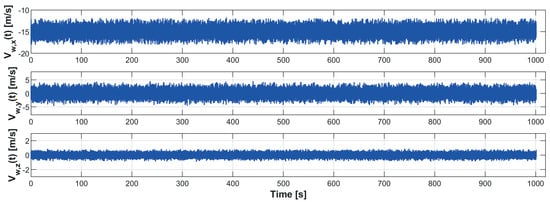
Figure A1.
Wind velocity in each Cartesian axis.
Figure A1.
Wind velocity in each Cartesian axis.
Appendix B. Linearized Model of the System
Appendix C. LQR Parameters
Appendix D. MPC Parameters
References
- Valavanis, K.P.; Vachtsevanos, G.J. Future of Unmanned Aviation. In Handbook of Unmanned Aerial Vehicles; Springer: Dordrecht, The Netherlands, 2015; pp. 2993–3009. [Google Scholar] [CrossRef]
- Microdrones. Unmanned Applied Solutions. 2020. Available online: https://www.microdrones.com/en/industry-experts/ (accessed on 14 November 2020).
- Roth, M. AI in Military Drones and UAVs—Current Applications. 2019. Available online: https://emerj.com/ai-sector-overviews/ai-drones-and-uavs-in-the-military-current-applications/ (accessed on 14 November 2020).
- Jerry, M. Current and future UAV military users and applications. Air Space Eur. 1999, 1, 51–58. [Google Scholar] [CrossRef]
- Geo-Matching. Aerial Imagery from UAVs. 2020. Available online: https://geo-matching.com/content/aerial-imagery-from-uavs (accessed on 14 November 2020).
- SenseFly. Why Use Drones For Environmental Monitoring? 2020. Available online: https://www.sensefly.com/industry/drones-environmental-monitoring/ (accessed on 14 November 2020).
- EKU. 5 Ways Drones Are Being Used for Disaster Relief. 2020. Available online: https://safetymanagement.eku.edu/blog/5-ways-drones-are-being-used-for-disaster-relief/ (accessed on 14 November 2020).
- Boeing. F-86 Sabre Jet—Historical Snapshot. 2020. Available online: https://www.boeing.com/history/products/f-86-sabre-jet.page (accessed on 14 November 2020).
- The Editors of Encyclopaedia Britannica. F-86. 2019. Available online: https://www.britannica.com/technology/F-86 (accessed on 14 November 2020).
- X-47B UCAS Unmanned Combat Air System. 2015. Available online: https://www.northropgrumman.com/what-we-do/air/x-47b-ucas/ (accessed on 14 November 2020).
- NavalTechnology. X-47B Unmanned Combat Air System (UCAS). 2016. Available online: https://www.naval-technology.com/projects/x-47b-unmanned-combat-air-system-carrier-ucas/ (accessed on 14 November 2020).
- Luo, C.; McClean, S.I.; Parr, G.; Teacy, L.; De Nardi, R. UAV position estimation and collision avoidance using the extended Kalman filter. IEEE Trans. Veh. Technol. 2013, 62, 2749–2762. [Google Scholar] [CrossRef]
- LaValle, S.M. Planning Algorithms; Cambridge University Press: Cambridge, UK, 2006; pp. 1–826. [Google Scholar] [CrossRef]
- Samaniego, F.; Sanchis, J.; Garcia-Nieto, S.; Simarro, R. Recursive Rewarding Modified Adaptive Cell Decomposition (RR-MACD): A Dynamic Path Planning Algorithm for UAVs. Electronics 2019, 8, 306. [Google Scholar] [CrossRef]
- Dijkstra, E.W. A note on two problems in connexion with graphs. Numer. Math. 1959, 1, 269–271. [Google Scholar] [CrossRef]
- Niu, L.; Zhuo, G. An Improved Real 3D a* Algorithm for Difficult Path Finding Situation. In Proceedings of the International Archives of the Photogrammetry, Remote Sensing and Spatial Information Sciences, Beijing, China, 3–11 July 2008; pp. 927–930. [Google Scholar]
- Ferguson, D.; Stentz, A. Field D*: An Interpolation-Based Path Planner and Replanner. In Robotics Research: Results of the 12th International Symposium, October 12–15, 2005, San Francisco, CA, USA; Springer: Berlin/Heidelberg, Germany, 2005; Volume 28, pp. 239–253. [Google Scholar] [CrossRef]
- De Filippis, L.; Guglieri, G.; Quagliotti, F. Path Planning Strategies for UAVS in 3D Environments. J. Intell. Robot. Syst. 2012, 65, 247–264. [Google Scholar] [CrossRef]
- Nakajima, K.; Premachandra, C.; Kato, K. 3D environment mapping and self-position estimation by a small flying robot mounted with a movable ultrasonic range sensor. J. Electr. Syst. Inf. Technol. 2017, 4, 289–298. [Google Scholar] [CrossRef]
- Premachandra, C.; Otsuka, M.; Gohara, R.; Ninomiya, T.; Kato, K. A study on development of a hybrid aerial/terrestrial robot system for avoiding ground obstacles by flight. IEEE/CAA J. Autom. Sin. 2019, 6, 327–336. [Google Scholar] [CrossRef]
- Premachandra, C.; Thanh, D.N.H.; Kimura, T.; Kawanaka, H. A study on hovering control of small aerial robot by sensing existing floor features. IEEE/CAA J. Autom. Sin. 2020, 7, 1016–1025. [Google Scholar] [CrossRef]
- Marco, V.; Contreras, R.; Sanchez, R.; Rodriguez, G.; Serrano, D.; Kerr, M.; Fernandez, V.; Haya-Ramos, R.; Peñin, L.F.; Ospina, J.A.; et al. The IXV guidance, navigation and control subsystem: Development, verification and performances. Acta Astronaut. 2016, 124, 53–66. [Google Scholar] [CrossRef]
- Premachandra, C.; Ueda, D.; Kato, K. Speed-Up Automatic Quadcopter Position Detection by Sensing Propeller Rotation. IEEE Sens. J. 2019, 19, 2758–2766. [Google Scholar] [CrossRef]
- Premachandra, C.; Otsuka, M. Development of hybrid aerial/terrestrial robot system and its automation. In Proceedings of the 2017 IEEE International Systems Engineering Symposium (ISSE), Vienna, Austria, 11–13 October 2017; pp. 1–3. [Google Scholar] [CrossRef]
- Pardo, C. Controlador PID. 2020. Available online: https://www.picuino.com/es/arduprog/control-pid.html (accessed on 14 November 2020).
- Fadali, M.S.; Visioli, A. Chapter 9—State Feedback Control. In Digital Control Engineering, 2nd ed.; Fadali, M.S., Visioli, A., Eds.; Academic Press: Boston, MA, USA, 2013; pp. 351–397. [Google Scholar] [CrossRef]
- Mathworks. Lqr. 2020. Available online: https://www.mathworks.com/help/control/ref/lqr.html (accessed on 14 November 2020).
- Hajiyev, C.; Soken, H.; Vural, S. Linear Quadratic Regulator Controller Design. In State Estimation and Control for Low-Cost Unmanned Aerial Vehicles; Springer: Berlin/Heidelberg, Germany, 2015; pp. 171–200. [Google Scholar] [CrossRef]
- Wang, L. Model Predictive Control System Design and Implementation Using MATLAB; Springer: London, UK, 2009; pp. 1–332. [Google Scholar] [CrossRef]
- Grancharova, A.; Johansen, T. Nonlinear Model Predictive Control. In Explicit Nonlinear Model Predictive Control; Grancharova, A., Johansen, T., Eds.; Springer: Berlin/Heidelberg, Germany, 2012; pp. 39–63. [Google Scholar] [CrossRef]
- Zhou, K.; Doyle, J.C. Essentials of Robust Control; Prentice Hall Upper Saddle River: New York, NY, USA, 1998; pp. 1–10. [Google Scholar]
- Gavilán, F.R. Sistemas de Control y Guiado para Vehículos Aéreos No Tripulados, Diseño de Algoritmos y Sistemas Embarcados. Ph.D. Thesis, University of Sevilla, Sevilla, Spain, 2012. [Google Scholar]
- Sujit, P.B.; Saripalli, S.; Sousa, J.B. An evaluation of UAV path following algorithms. In Proceedings of the 2013 European Control Conference (ECC), Zurich, Switzerland, 17–19 July 2013; pp. 3332–3337. [Google Scholar] [CrossRef]
- Espinoza-Fraire, T.; Dzul, A.; Cortés-Martínez, F.; Giernacki, W. Real-time implementation and flight tests using linear and nonlinear controllers for a fixed-wing miniature aerial vehicle (MAV). Int. J. Control Autom. Syst. 2018, 16, 392–396. [Google Scholar] [CrossRef]
- Bulka, E.; Nahon, M. Autonomous fixed-wing aerobatics: From theory to flight. In Proceedings of the 2018 IEEE International Conference on Robotics and Automation (ICRA), Brisbane, Australia, 21–25 May 2018; pp. 6573–6580. [Google Scholar]
- Kamel, M.; Stastny, T.; Alexis, K.; Siegwart, R. Model predictive control for trajectory tracking of unmanned aerial vehicles using robot operating system. In Robot Operating System (ROS); Springer: Berlin/Heidelberg, Germany, 2017; pp. 3–39. [Google Scholar]
- Stastny, T.J.; Dash, A.; Siegwart, R. Nonlinear MPC for fixed-wing UAV trajectory tracking: Implementation and flight experiments. In Proceedings of the Aiaa Guidance, Navigation, and Control Conference, Grapevine, TX, USA, 9–13 January 2017; p. 1512. [Google Scholar]
- Department of Defense of the United States of America. OP 1280. Declassification. 1955. Available online: https://fdocuments.in/document/op-1280-aircraft-bombs.html (accessed on 14 November 2020).
- United States Air Force. Handbook Maintenance Instructions USAF Series F-86F Aircraft. Declassification. 1954. Available online: https://www.avialogs.com/aircraft-n/north-american-aviation/item/55493-t-o-1f-86f-2-handbook-maintenance-instructions-f-86f-aircraft (accessed on 14 November 2020).
- United States Air Force. Flight Manual USAF Series F-86F Aircraft. Declassification. 1960. Available online: https://www.esscoaircraft.com/p-9741-north-american-f-86f-1960-flight-manual.aspx (accessed on 14 November 2020).
- Cook, M. Flight Dynamics Principles, 3rd ed.; Butterworth-Heinemann: Cranfield, UK, 2013; pp. 1–145. [Google Scholar] [CrossRef]
- Napolitano, M. Aircraft Dynamics: From Modeling to Simulation; John Wiley & Sons, Inc.: Morgantown, WV, USA, 2012; pp. 135–267. [Google Scholar]
- Magraner Rullan, J.P.; Carreres Talens, M.; Martí Gómez-Aldaraví, P. Flight Mechanics; Universitat Politècnica de València: Valencia, Spain, 2018; pp. 1–190. [Google Scholar] [CrossRef]
- Roux, É. Turbofan and Turbojet Engines: Database Handbook; Élodie Roux: Blagnac, France, 2007; p. 242. [Google Scholar]
- Ortiz, Á. Design and Simulation of the Guidance and Control System for an F-86 Sabre. Bachelor’s Thesis, Universitat Politècnica de València, Valencian Community, Spain, 2020. Available online: http://hdl.handle.net/10251/153251 (accessed on 14 November 2020).
- Sumair, M.; Aized, T.; Gardezi, S.A.R.; Bhutta, M.M.A.; Rehman, S.M.S.; ur Rehman, S.U. Application of five continuous distributions and evaluation of wind potential at five stations using normal distribution. Energy Explor. Exploit. 2020, 1–3. [Google Scholar] [CrossRef]
- Yuan, K.; Zhang, K.; Zheng, Y.; Li, D.; Wang, Y.; Yang, Z. Irregular distribution of wind power prediction. J. Mod. Power Syst. Clean Energy 2018, 6, 1172–1180. [Google Scholar] [CrossRef]
- Bryc, W. The Normal Distribution, 1st ed.; Springer: New York, NY, USA, 1995; pp. 23–28. [Google Scholar]
- El Dorado Weather. Alaska Mean Wind Speed and Prevailing Direction. 2020. Available online: https://www.eldoradoweather.com/ (accessed on 14 November 2020).
- Weather Spark. The Typical Weather Anywhere on Earth. 2020. Available online: https://weatherspark.com/ (accessed on 14 November 2020).
- SKYbrary. International Standard Atmosphere (ISA). 2017. Available online: https://www.skybrary.aero/index.php/International_Standard_Atmosphere_(ISA) (accessed on 14 November 2020).
- Steve, A. International Standard Atmosphere: How it Affects Flight—Understanding the Basics. 2014. Available online: https://www.universalweather.com/blog/international-standard-atmosphere-how-it-affects-flight-understanding-the-basics/ (accessed on 14 November 2020).
- U.S. Department of the Interior. What Are Digital Elevation Models (DEMs)? 2020. Available online: https://www.usgs.gov/ (accessed on 14 November 2020).
- NRC Services. National Elevation Dataset. 2020. Available online: https://www.usda.gov/ (accessed on 14 November 2020).
- U.S. Department of the Interior. The National Map. 2020. Available online: https://www.usgs.gov/core-science-systems/national-geospatial-program/national-map (accessed on 14 November 2020).
- Arms, C.R.; Fleischhauer, C.; Murray, K. KML, Version 2.2. 2012. Available online: https://www.loc.gov/preservation/digital/formats/fdd/fdd000340.shtml (accessed on 14 November 2020).
- Schneider, A. GPS Visualizer: Do-It-Yourself Mapping. 2019. Available online: https://www.gpsvisualizer.com/ (accessed on 14 November 2020).
- Hazzard, C. What is a GPX File? 2020. Available online: https://hikingguy.com/how-to-hike/what-is-a-gpx-file/ (accessed on 14 November 2020).
- Thompson, W. F-86 Sabre Fighter-Bomber Units Over Korea; Osprey Publishing: Oxford, UK, 1999; pp. 8–73. [Google Scholar]
- History.com Editors. Korean War. 2020. Available online: https://www.history.com/topics/korea/korean-war (accessed on 14 November 2020).
- Samet, H.; Kochut, A. Octree approximation an compression methods. In Proceedings of the 1st International Symposium on 3D Data Processing Visualization and Transmission, Padova, Italy, 19–21 June 2002; pp. 460–469. [Google Scholar] [CrossRef]
- Samaniego, F.; Sanchis, J.; Garcia-Nieto, S.; Simarro, R. Smooth 3D Path Planning by Means of Multiobjective Optimization for Fixed-Wing UAVs. Electronics 2019, 9, 51. [Google Scholar] [CrossRef]
- Oshana, R. 4—Overview of Digital Signal Processing Algorithms. In DSP Software Development Techniques for Embedded and Real-Time Systems; Oshana, R., Ed.; Embedded Technology, Newnes: Burlington, MA, USA, 2006; pp. 59–121. [Google Scholar] [CrossRef]
- Anjali, B.; Vivek, A.; Nandagopal, J. Simulation and analysis of integral LQR controller for inner control loop design of a fixed wing micro aerial vehicle (MAV). Procedia Technol. 2016, 25, 76–83. [Google Scholar] [CrossRef][Green Version]
- Boyd, S.; El Ghaoui, L.; Feron, E.; Balakrishnan, V. Linear Matrix Inequalities in System and Control Theory; Society for Industrial and Applied Mathematics: Philadelphia, PA, USA, 1994. [Google Scholar] [CrossRef]
- Maciejowski, J. Predictive Control: With Constraints, 1st ed.; Prentice Hall: London, UK, 2002. [Google Scholar]
- Cuzzola, F.A.; Geromel, J.C.; Morari, M. An Improved Approach for Constrained Robust Model Predictive Control. Automatica 2002, 38, 1183–1189. [Google Scholar] [CrossRef]
- Maeder, U.; Borrelli, F.; Morari, M. Linear Offset-Free Model Predictive Control. Automatica 2009, 45, 2214–2222. [Google Scholar] [CrossRef]
- Mayne, D.; Rawlings, J.; Rao, C.; Scokaert, P. Constrained Model Predictive Control: Stability and Optimality. Automatica 2000, 36, 789–814. [Google Scholar] [CrossRef]
- Mayne, D.Q. Model Predictive Control: Recent Developments and Future Promise. Automatica 2014, 50, 2967–2986. [Google Scholar] [CrossRef]
- Kouvaritakis, B.; Cannon, M. Model Predictive Control. Classical, Robust and Stochastic, 1st ed.; Springer International Publishing: Berlin/Heidelberg, Germany, 2016. [Google Scholar] [CrossRef]
- Blanchini, F.; Miani, S. Set-Theoretic Methods in Control, 1st ed.; Birkhäuser: Boston, MA, USA, 2008. [Google Scholar] [CrossRef]
- Khlebnikov, M.V.; Polyak, B.T.; Kuntsevich, V.M. Optimization of Linear Systems Subject to Bounded Exogenous Disturbances: The Invariant Ellipsoid Technique. Autom. Remote Control 2011, 72, 2227–2275. [Google Scholar] [CrossRef]
- Ortiz, Á. Autonomous Navigation for an F-86 Sabre. 2021. Available online: https://es.mathworks.com/matlabcentral/fileexchange/85168-autonomous-navigation-system-for-an-f-86-sabre (accessed on 14 November 2020).
- Fleeman, E.L. Tactical Missile Design, 2nd ed.; American Institute of Aeronautics and Astronautics: Atlanta, GA, USA, 2006; pp. 21–80. [Google Scholar]
- Blog, T.S.C. Coding Bilinear Interpolation. 2011. Available online: http://supercomputingblog.com/graphics/coding-bilinear-interpolation/ (accessed on 14 November 2020).
- Cutler, C. Ground Effect: Why You Float During Landing. 2020. Available online: https://www.boldmethod.com/learn-to-fly/aerodynamics/what-happens-to-your-plane-in-ground-effect/ (accessed on 14 November 2020).
- Airport Authorities India. What Is an ILS and Its Different Component? 2020. Available online: https://www.aai.aero/en/content/what-ils-and-its-different-component (accessed on 14 November 2020).
- Demirhan, M.; Premachandra, C. Development of an Automated Camera-Based Drone Landing System. IEEE Access 2020, 8, 202111–202121. [Google Scholar] [CrossRef]
- Bouhali, M.; Shamani, F.; Dahmane, Z.E.; Belaidi, A.; Nurmi, J. FPGA applications in unmanned aerial vehicles—A review. In International Symposium on Applied Reconfigurable Computing; Springer: Berlin/Heidelberg, Germany, 2017; pp. 217–228. [Google Scholar]
- Kunzler, J.W.; Ammermon, S.M.; Warnick, K.F. Progress Toward Airborne GPS Spatial Filtering Powered by Recent Advances in FPGA Technology. In Proceedings of the 2020 Intermountain Engineering, Technology and Computing (IETC), Orem, UT, USA, 2–3 October 2020; pp. 1–6. [Google Scholar]
Publisher’s Note: MDPI stays neutral with regard to jurisdictional claims in published maps and institutional affiliations. |
© 2021 by the authors. Licensee MDPI, Basel, Switzerland. This article is an open access article distributed under the terms and conditions of the Creative Commons Attribution (CC BY) license (http://creativecommons.org/licenses/by/4.0/).


