Wind Turbine Operation Curves Modelling Techniques

Abstract

Wind turbines are machines operating in non-stationary conditions and the power of a wind turbine depends non-trivially on environmental conditions and working parameters. For these reasons, wind turbine power monitoring is a complex task which is typically addressed through data-driven methods for constructing a normal behavior model. On these grounds, this study is devoted the analysis of meaningful operation curves, which are rotor speed-power, generator speed-power and blade pitch-power. A key point is that these curves are analyzed in the appropriate operation region of the wind turbines: the rotor and generator curves are considered for moderate wind speed, when the blade pitch is fixed and the rotational speed varies (Region 2); the blade pitch curve is considered for higher wind speed, when the rotational speed is rated (Region 2 $\raisebox{1ex}{$1$}\!\left/ \!\raisebox{-1ex}{$2$}\right.$). The selected curves are studied through a multivariate Support Vector Regression with Gaussian Kernel on the Supervisory Control And Data Acquisition (SCADA) data of two wind farms sited in Italy, featuring in total 15 2 MW wind turbines. An innovative aspect of the selected models is that minimum, maximum and standard deviation of the independent variables of interest are fed as input to the models, in addition to the typically employed average values: using the additional covariates proposed in this work, the error metrics decrease of order of one third, with respect to what would be obtained by employing as regressors only the average values of the independent variables. In general it results that, for all the considered curves, the prediction of the power is characterized by error metrics which are competitive with the state of the art in the literature for multivariate wind turbine power curve analysis: in particular, for one test case, a mean absolute percentage error of order of 2.5% is achieved. Furthermore, the approach presented in this study provides a superior capability of interpreting wind turbine performance in terms of the behavior of the main sub-components and eliminates as much as possible the dependence on nacelle anemometer data, whose use is critical because of issues related to the sites complexity.

1. Introduction

Operation and maintenance of wind turbines represent an important fraction (up to 20–25%) of the life-cycle costs of an industrial plant. Furthermore the recent trends about increasing rotor sizes [1,2] and offshore exploitation [3,4,5] complicate the accessibility to wind turbine sites and increase the intervention costs in case of unexpected wind turbine stops.

For these reasons, and also in light of the non-stationary conditions to which wind turbines are subjected, remote control and monitoring [6,7] of wind farms is an objective whose importance has been continuously growing. Fortunately, the widespread diffusion of Supervisory Control And Data Acquisition (SCADA) control systems and of Turbine Condition Monitoring (TCM) systems guarantees the availability of most of the data which are necessary for wind turbine control and monitoring. Nevertheless, transforming the available information into knowledge about the health status or the performance of wind turbines is particularly complex. For example, as regards the detection of mechanical damages at gears and bearings through vibration data analysis, it is prohibitive to isolate the signatures associated to incoming faults [8,9,10,11].

As regards the monitoring of wind turbine performance, the main issue is that a wind turbine has a multivariate dependence on environmental conditions [12,13] and working parameters. SCADA control systems typically record and store (with some minutes of sampling time) the main working parameters and also internal temperatures collected at meaningful wind turbine sub-components. By this point of view, therefore, the main issue is incorporating efficiently this kind of information for constructing normal behavior models for the performance of the wind turbines [14,15,16,17], which can useful as well for condition monitoring purposes [18,19].

The simplest data-driven model employed for wind turbine performance monitoring is the power curve [20,21,22,23], which is the relation between the average wind speed and the extracted power. On the grounds of the above discussion, a recent trend in wind energy literature regards multivariate approaches to the power curve: in [24,25,26], the point of view is including additional environmental variables (either measured ambient temperature, humidity, and wind direction as in [24] or estimated by a Numerical Weather Prediction model as in [25]); in [27,28,29,30], the approach consists in including the most important operation variables (as the blade pitch and the rotor speed) in the multivariate modelling of the power curve.

An interesting approach to wind turbine power monitoring consists in the analysis of other operation curves, mainly regarding the rotor speed and the blade pitch. In [31,32], the wind speed-blade pitch curve of wind turbines is analyzed using Support Vector Regression and the results are compared against the binning method. In [33], two fundamental operation curves are analyzed through Gaussian process methods: the wind speed-blade pitch and the wind speed-rotor speed curves.

A further development of these concepts regards the analysis of operation curves which do not involve the wind speed measured at the nacelle of the wind turbines. The rationale for this consideration is that in general the nacelle wind speed is measured behind the rotor span and the undisturbed wind speed is estimated through a nacelle transfer function: this introduces possible drawbacks, especially in complex environment. Furthermore, it is not rare that nacelle anemometers are subjected to failures or bias [34]. These considerations have even led to the formulation of the concept of rotor equivalent wind speed [35,36]: the idea is that, since the rotor speed is controlled on the grounds on the torque and not on the grounds of the nacelle anemometer, the rotor itself can be considered as a probe for estimating the wind speed.

Therefore, this study is devoted to the data-driven analysis of three operation curves, which are rotor speed-power, generator speed-power and blade pitch-power curve. To best of the author’s knowledge, despite the potential interest of these curves in wind turbine power monitoring, this topic has not been addressed systematically in the literature, except for the intuition contained in [37], regarding the fact these curves can be particularly meaningful for wind turbine aging estimation.

The objective of this study is formulating a methodology for monitoring the performance of wind turbines using the above indicated curves: this in practice has been realized by verifying the robustness of a non-linear multivariate regression, which can therefore be employed as a normal behavior model for comparing the expected performance against the actual performance.

The data analysis is appropriately conducted in light of the principles of the control of wind turbines: for moderate wind speed (approximately between 5 m/s and 9 m/s), the blade pitch is kept fixed and the wind turbine attains the highest possible aerodynamic efficiency by regulating the rotor speed; for higher wind speed (approximately between 9 m/s and 13 m/s), the wind turbine operates in partial aerodynamic load by keeping constant the rotational speed and by regulating the blade pitch. These two operation regions are typically overall indicated as Region 2 of the power curve of a wind turbine, because they are between cut-in and rated: in [37], in order to distinguish them, they are indicated as Region 2 and Region 2 $\raisebox{1ex}{$1$}\!\left/ \!\raisebox{-1ex}{$2$}\right.$ and the same notation is employed in this study. Therefore, in this work, the selected operation curves are analyzed in the regions where they are of most interest for performance monitoring purposes: rotor and generator speed curves in Region 2, blade pitch curve in Region 2 $\raisebox{1ex}{$1$}\!\left/ \!\raisebox{-1ex}{$2$}\right.$. The interest for the blade pitch-power curve regards also the fact that, when the rotor speed saturates, the rotor equivalent wind speed becomes meaningless and therefore it is conceivable to use the blade pitch curve as the basis for a sort of pitch equivalent wind speed.

Due to the non-linear relation between the input variables and the power output, the selected methodology for the analysis of the curves is a Support Vector Regression with Gaussian Kernel. An innovative aspect of this study deals with the selection of the set of covariates for the regression. In the literature about wind turbine power monitoring, it is typical that the selected covariates are the average values as stored by the SCADA control system, but it should be noticed that SCADA systems store as well the minimum, the maximum and the standard deviation in the sampling interval for each measured channel. In this study, the possibility has been explored of including also minimum, maximum and standard deviation of the selected input variables, in order to inquire within what extent the normal behavior model improves. Sideways, this simple idea, which is enriching the covariates structure rather than complicating the model structure, could be inspiring for multivariate power curve modelling because the critical point is exactly reproducing the observed variability of the extracted power, given average conditions.

The main result of this work therefore consists in the verification that, using the proposed methodology, it is possible to model the power of a wind turbine with a precision which is competitive with the state of the art in the literature, but without using the nacelle wind speed as input variable: this is definitely non-trivial because, as discussed for example in [27], the wind speed explains up to 98% of the variance of the power of a wind turbine.

Summarizing, the structure of the manuscript is therefore the following: in Section 2, the test case and the data sets used for the present study are described; Section 3 is devoted to the methods; the results are collected and discussed in Section 4; conclusions are drawn and further directions of the present work are indicated in Section 5.

2. The Test Cases

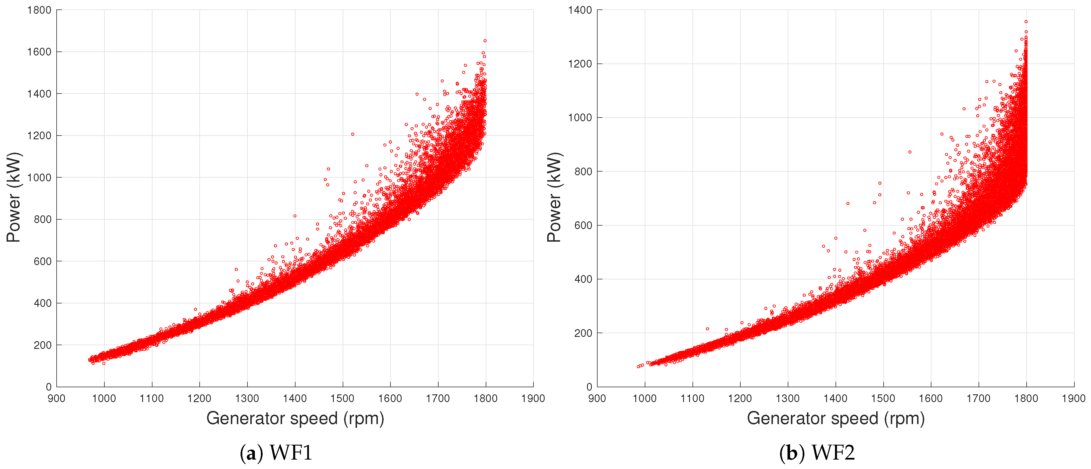
The selected test cases were two wind farms (named as WF1 and WF2) sited in southern Italy on gentle terrains, featuring respectively six and nine wind turbines whose rated power was 2 MW. The rotor diameters at WF1 was 92 m and at WF2 was 82 m. The layouts are reported in Figure 1 and Figure 2: from these Figures it arises that the interturbine distance at WF1 was considerably higher with respect to WF2. Therefore, the impact of wakes on wind turbine operation was low for WF1, while it was relevant for WF2 (as discussed, for example, in [38,39]).

Operation data spanning the years 2017 and 2018 were used, courtesy of the ENGIE Italia company. The measurements used were the following:

• nacelle wind speed v;
• power production P;
• blade pitch $\beta$;
• rotor speed $\Omega$;
• generator speed $\omega$.

The data had 10 min of sampling time. For each channel, average, minimum, maximum and standard deviation over the 10 min interval have been used.

Data were pre-processed by filtering on wind turbine operation using the appropriate run time counter available in the SCADA data set. Subsequently, each data set was divided according to the operation region, as indicated in

Table 1. Operation regions for the test case wind turbine.

Region	Condition
2	$5\le v\le 9$
2 $\raisebox{1ex}{$1$}\!\left/ \!\raisebox{-1ex}{$2$}\right.$	$9<v\le 13$

, on the grounds of nacelle wind intensity v. The same notation as in [37] was adopted: the regime when the wind turbine operated at full aerodynamic load, with variable rotational speed and fixed pitch, is indicated as Region 2; instead, the regime characterized by rated rotational speed and variable pitch is indicated as Region 2 $\raisebox{1ex}{$1$}\!\left/ \!\raisebox{-1ex}{$2$}\right.$.

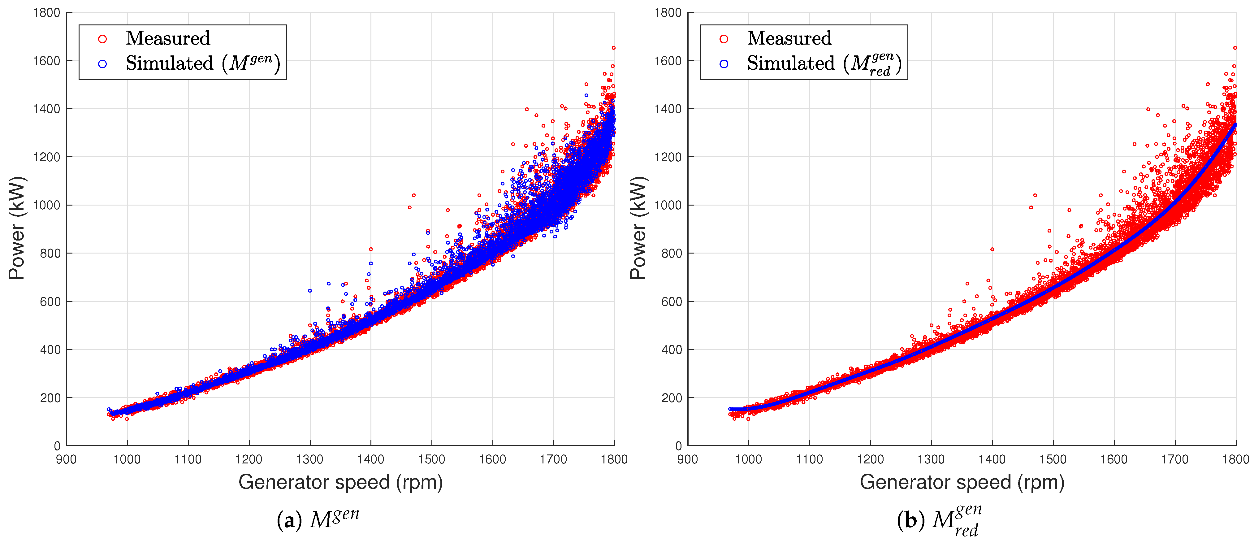
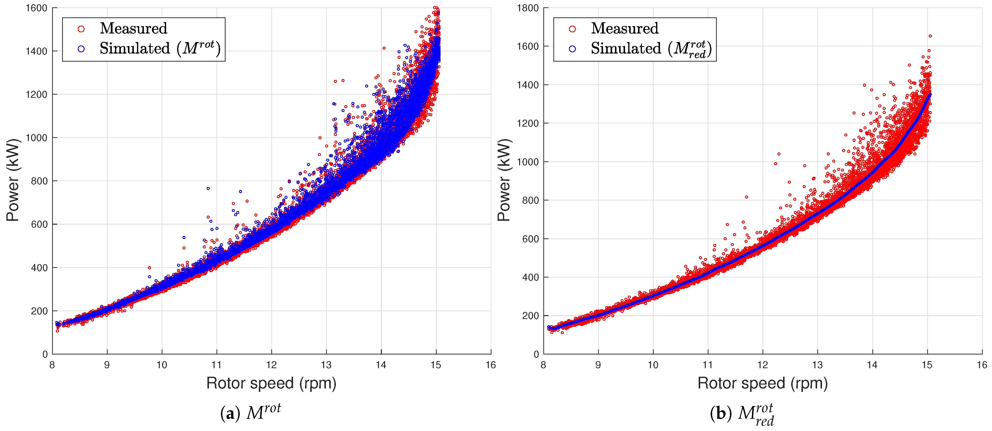
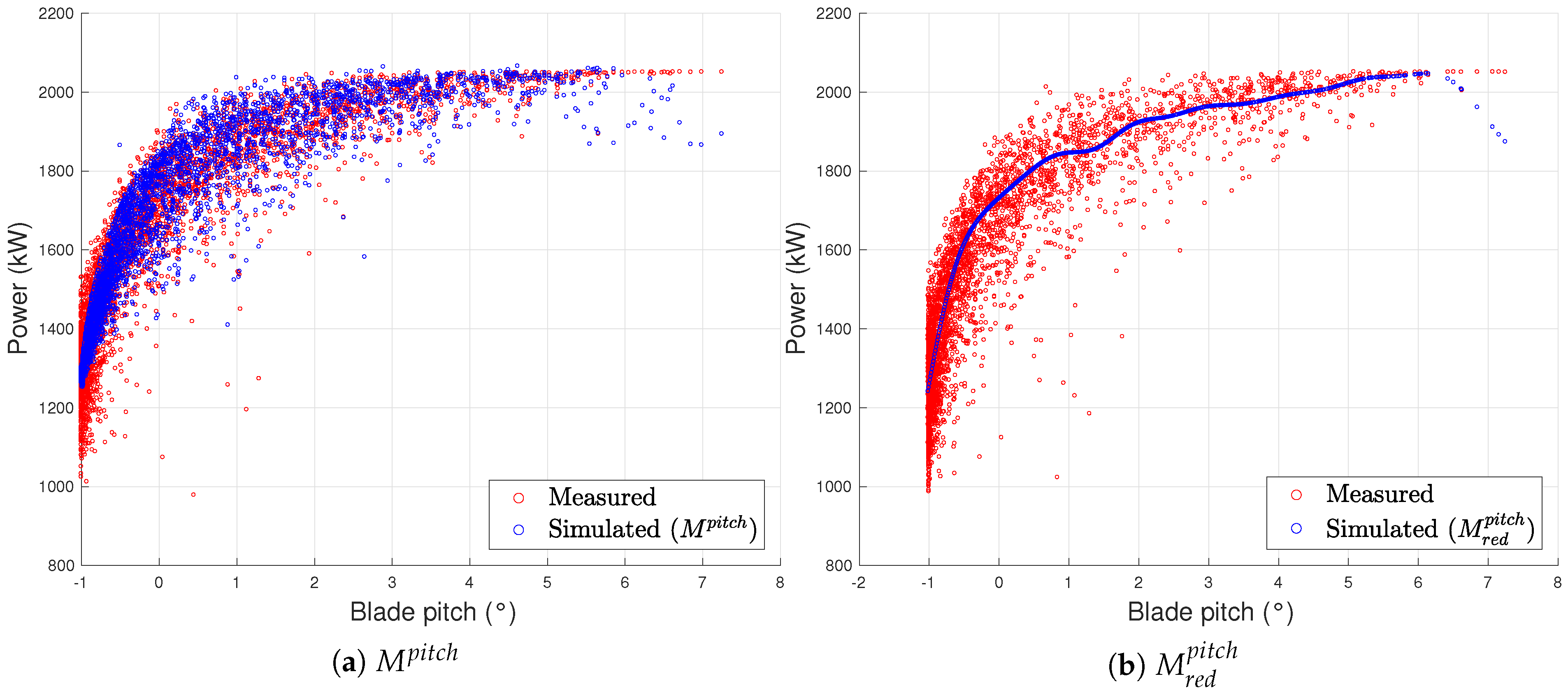
Examples of the operation curves under analysis were reported for a sample wind turbine (T1) for each test case in Figure 3 (generator speed-power), Figure 4 (rotor speed-power) and Figure 5 (blade pitch-power): from these Figures, it arises that the curves were qualitatively similar and therefore the logic of the control was the same.

3. The Method

The objective of the study was formulating a reliable methodology for wind turbine power monitoring using the selected operation curves, depending on the working region. This passes through the construction of a normal behavior model for the curves and consequently consists in the comparison between the model estimates and the measurements in the validation data set. In this study, a Support Vector Regression with Gaussian Kernel was selected for constructing the normal behavior models because this kind of regression has proven to be effective for multivariate modeling of wind turbine power [37,40]. In the following, therefore, the general principles of the Support Vector Regression are briefly recapped and, subsequently, it will be discussed how to apply them for monitoring the operation curves of interest.

Given a matrix $\mathit{X}$ of input variables, where the covariates are grouped according to the columns and the observations are grouped according to the rows, a linear model is posed in Equation (1):

$$f\left(\mathit{X}\right)=\mathit{X}\mathit{\beta }+\mathit{b},$$

(1)

where $\mathit{\beta }$ is the vector of regression coefficients and $\mathit{b}$ is the intercept vector.

The Support Vector Regression consists in a methodology for estimating the $\mathit{\beta }$ parameters. It relies on the constraint that the residuals between the measurement Y and the model estimate $f\left(\mathit{X}\right)$ are lower than a threshold $ϵ$ for each n-th observation Equation (16):

$$\left|Y_n-{\mathit{X}}_n\mathit{\beta }+b_n\right|\le ϵ.$$

(2)

The optimization problem can be rephrased in the Lagrange dual formulation; the function to minimize is $L\left(\alpha \right)$, given in Equation (3):

$$L\left(\alpha \right)=\frac{1}{2}\sum _{i=1}^N\sum _{j=1}^N\left({\alpha }_i-{\alpha }_i^{*}\right)\left({\alpha }_j-{\alpha }_j^{*}\right){\mathit{X}}_i^{\prime }{\mathit{X}}_j+ϵ\sum _{i=1}^N\left({\alpha }_i+{\alpha }_i^{*}\right)+\sum _{i=1}^N{Y}_i\left({\alpha }_i^{*}-{\alpha }_i\right),$$

(3)

with the constraints Equation (4)

$$\begin{array}{c}\hfill {\displaystyle \sum _{n=1}^N}\left({\alpha }_n-{\alpha }_n^{*}\right)=0\\ \hfill 0\le {\alpha }_n\le C\\ \hfill 0\le {\alpha }_n^{*}\le C,\end{array}$$

(4)

where C is the box constraint.

The solution for the $\mathit{\beta }$ parameters in terms of the observations matrix $\mathit{X}$ and of ${\alpha }_n$ or ${\alpha }_n^{*}$ is given in Equation (5):

$$\mathit{\beta }=\sum _{n=1}^N\left({\alpha }_n-{\alpha }_n^{*}\right){\mathit{X}}_n.$$

(5)

In a nutshell, the optimization passes through the data-driven selection of the most meaningful rows of the observations matrix $\mathit{X}$, which for this reason are named support vectors and which are weighted through the ${\alpha }_n$ or ${\alpha }_n^{*}$ coefficients.

Once the $\mathit{\beta }$ coefficients have been computed on a reference data set, they can be used for predicting new values through Equation (6), given the input variables matrix $\mathit{X}$:

$$f\left(\mathit{X}\right)=\sum _{n=1}^N\left({\alpha }_n-{\alpha }_n^{*}\right){\mathit{X}}_n^{\prime }\mathit{X}+\mathit{b}.$$

(6)

The non-linear Support Vector Regression is obtained by replacing the products between the observations matrix with a non-linear Kernel function Equation (7):

$$G\left({\mathit{X}}_1,{\mathit{X}}_2\right)=\langle \phi \left({\mathit{X}}_1\right)\phi \left({\mathit{X}}_2\right)\rangle ,$$

(7)

where $\phi$ is a transformation mapping the $\mathit{X}$ observations into the feature space.

A Gaussian Kernel selection is given in Equation (8) and has been widely employed in wind energy literature for non-linear regression problems [31]:

$$G\left({\mathit{X}}_i,{\mathit{X}}_j\right)=e^{-\kappa {∥{\mathit{X}}_i-{\mathit{X}}_j∥}^2},$$

(8)

where $\kappa$ is the Kernel scale.

Then Equation (3) rewrites as in Equation (9):

$$L\left(\alpha \right)=\frac{1}{2}\sum _{i=1}^N\sum _{j=1}^N\left({\alpha }_i-{\alpha }_i^{*}\right)\left({\alpha }_j-{\alpha }_j^{*}\right)G\left({\mathit{X}}_i,{\mathit{X}}_j\right)+ϵ\sum _{i=1}^N\left({\alpha }_i+{\alpha }_i^{*}\right)+\sum _{i=1}^N{Y}_i\left({\alpha }_i^{*}-{\alpha }_i\right),$$

(9)

and Equation (6) for predicting rewrites as in Equation (10):

$$f\left(\mathit{X}\right)=\sum _{n=1}^N\left({\alpha }_n-{\alpha }_n^{*}\right)G\left({\mathit{X}}_n,\mathit{X}\right)+\mathit{b}.$$

(10)

In this work, the hyperparameters of the regression $\kappa$, C, $ϵ$ have been automatically optimized, basing on the evaluation on 30 model calls of the cross-validation loss.

In order to appreciate the usefulness of the selected non-linear regression for the problem of this study, a comparison is set up against a multivariate linear model: Principal Component Regression [41].

The ordinary least squares estimate of the linear model coefficients Equation (1) is given in Equation (11):

$${\mathit{\beta }}_{ols}={\left({\mathit{X}}^T\mathit{X}\right)}^{-1}{\mathit{X}}^{T}Y.$$

(11)

If the input variables of the matrix $\mathit{X}$ are strongly correlated, the estimate of the $\mathit{\beta }$ coefficients is affected by large uncertainty: for this reason, the idea of of the Principal Component Regression is constructing an input variables matrix having mutually orthogonal columns.

Given the singular value decomposition of $\mathit{X}$ in Equation (12)

$$\mathit{x}=\mathit{U}\Delta {\mathit{V}}^T,$$

(12)

the columns of $\mathit{U}$ and $\mathit{V}$ are orthonormal sets of vectors denoting the left and right singular vectors of $\mathit{X}$ and $\Delta$ is a diagonal matrix, whose elements are the singular values of $\mathit{X}$.

Therefore, the matrix $\mathit{X}{\mathit{X}}^T$ can be decomposed as:

$$\mathit{X}{\mathit{X}}^T=\mathit{V}\Lambda {\mathit{V}}^T,$$

(13)

where $\Lambda =diag\left({\lambda }_1,\dots ,{\lambda }_p\right)$ and ${\lambda }_1\ge \dots \ge {\lambda }_p\ge 0$.

The Principal Component Regression poses an ordinary least squares model between the transformed data matrix $\mathit{W}=\mathit{x}\mathit{V}$ and the target Y. Therefore, the estimate of $\mathit{\beta }$ is given in Equation (14):

$${\mathit{\beta }}_{PCR}=\mathit{V}{\left({\mathit{W}}^T\mathit{W}\right)}^{-1}{\mathit{W}}^{T}Y.$$

(14)

Once ${\mathit{\beta }}_{PCR}$ has been calculated using training data, the model can be used for predicting through Equation (15):

$$f\left(\mathit{X}\right)=\mathit{X}{\mathit{\beta }}_{PCR},$$

(15)

which is the corresponding of Equation (10) for the Principal Component Regression.

The data sets used for this study were employed as follows for the regression:

• The data from the year 2017 were used for optimizing and training the regression and are named as D1;
• The validation data set D2 was constituted by the data from the 2018.

The quality of the regression was analyzed through common error metrics, which were the Mean Absolute Error ($MAE$), Mean Absolute Percentage Error ($MAPE$) and Root Mean Square Error ($RMSE$).

Given the measurements $Y\left(\mathit{X}\right)$ for the data set D2 and the model estimates $f\left(\mathit{X}\right)$, the residuals are defined in Equation (16):

$$R\left(\mathit{X}\right)=Y\left(\mathit{X}\right)-f\left(\mathit{X}\right).$$

(16)

The MAE is defined in Equation (17):

$$MAE=\frac{1}{N}\sum \left|R\left(\mathit{X}\right)\right|,$$

(17)

where N is the number of samples in the D2 data set. The MAPE is defined in Equation (18):

$$MAPE=\frac{100}{N}\sum \left|\frac{R\left(\mathit{X}\right)}{Y\left(\mathit{X}\right)}\right|$$

(18)

and the $RMSE$ is defined in Equation (19):

$$RMSE=\sqrt{\frac{\sum {\left(R\left(\mathit{X}\right)-\overline{R}\right)}^2}{N}},$$

(19)

where $\overline{R}$ is the average residual in the data set D2.

Finally, the selected structure of the regression was the following: for each curve, the columns of the $\mathit{X}$ matrix were constituted by the corresponding independent variable (generator speed, rotor speed, blade pitch respectively). The main novelty proposed in this manuscript as regards covariates selection was to include also the minimum, maximum and standard deviation as further regressors in addition to the average value. Therefore for, say, the generator speed-power curve regression, the $\mathit{X}$ matrix was constituted by average, minimum, maximum, standard deviation of the generator speed and the output Y will be the power P. In the following, this kind of model will be indicated as M. In order to provide a benchmark more in line with previous findings in the literature, a reduced model (indicated as $M_{red}$) was analyzed as well: in this case, the unique covariate was the average value of the independent variable of interest (for example, the generator speed for the generator speed-power curve) and therefore the model was univariate non-linear. Furthermore, for the M multivariate models, the Support Vector Regression and the Principal Component Regression were set up and the results were compared, while the univariate linear model was discarded because it was too simple for the problem. Summarizing, for each curve a comparison of univariate and multivariate non-linear models was performed (M against $M_{red}$), in order to appreciate the importance of the additional covariates selection proposed in this study. Furthermore, for the multivariate models, a comparison of non-linear (Support Vector) and linear (Principal Component) regression was performed, in order to appreciate the importance of non-linearity. Therefore, the structure of the employed regressions is summarized in

Table 2. The structure of the regressions.

Curve	Model	Types	Regressors
Generator	$M^{gen}$	SVR and PCR	Generator speed $\omega$ (average, min, max, std. dev)
Generator	$M_{red}^{gen}$	SVR	Generator speed $\omega$ (average)
Rotor	$M^{rot}$	SVR and PCR	Rotor speed $\Omega$ (average, min, max, std. dev)
Rotor	$M_{red}^{rot}$	SVR	Rotor speed $\Omega$ (average)
Pitch	$M^{pitch}$	SVR and PCR	Blade pitch $\beta$ (average, min, max, std. dev)
Pitch	$M_{red}^{pitch}$	PCR	Blade pitch $\beta$ (average)

.

4. Results

4.1. WF1

In Figure 6, Figure 7 and Figure 8, examples of measured and simulated curves are reported. The results for the complete models M are reported on the left, while on the right the results for the corresponding reduced models $M_{red}$ are reported. A sample wind turbine (T1) was selected and the employed data set was the validation one (D2). As regards all the curves, it arises that the full models M were more capable of reproducing the actual dispersion of the measured curves: therefore, the inclusion of the minimum, maximum and standard deviation of the input as further covariates for the regression proved to be decisive for a more realistic modelling of the curves.

The qualitative results of Figure 6, Figure 7 and Figure 8 were confirmed by the quantitative analysis reported in

Table 3. Results of the models validation for the generator speed-power curve in Region 2.

Model	Metric	T1	T2	T3	T4	T5	T6
$M^{gen}$	$MAE$ (kW)	13.8	16.7	17.4	18.2	17.5	15.6
$M_{red}^{gen}$	$MAE$ (kW)	22.7	24.8	23.7	27.9	24.6	21.4
$M^{gen}$	$RMSE$ (kW)	23.8	26.9	30.9	30.3	27.1	25.5
$M_{red}^{gen}$	$RMSE$ (kW)	39.6	43.2	41.0	50.8	44.1	39.6
$M^{gen}$	$MAPE$ (%)	2.2	2.6	2.8	2.7	2.7	2.4
$M_{red}^{gen}$	$MAPE$ (%)	3.5	3.6	3.7	3.7	3.4	3.0

,

Table 4. Results of the models validation for the rotor speed-power curve in Region 2: WF1.

Model	Metric	T1	T2	T3	T4	T5	T6
$M^{rot}$	$MAE$ (kW)	13.4	17.3	17.5	18.4	17.5	15.5
$M_{red}^{rot}$	$MAE$ (kW)	20.4	23.6	22.3	27.4	26.5	21.4
$M^{rot}$	$RMSE$ (kW)	23.3	28.0	30.9	30.6	27.2	25.7
$M_{red}^{rot}$	$RMSE$ (kW)	39.4	43.2	40.7	50.8	44.0	39.5
$M^{rot}$	$MAPE$ (%)	2.3	2.6	2.8	2.7	2.7	2.4
$M_{red}^{rot}$	$MAPE$ (%)	2.9	3.3	3.4	3.5	3.9	3.0

and

Table 5. Results of the models validation for the blade pitch-power curve in Region 2 $\raisebox{1ex}{$1$}\!\left/ \!\raisebox{-1ex}{$2$}\right.$: WF1.

Model	Metric	T1	T2	T3	T4	T5	T6
$M^{pitch}$	$MAE$ (kW)	44.2	50.9	52.1	47.0	51.4	42.8
$M_{red}^{pitch}$	$MAE$ (kW)	67.7	68.8	76.9	72.4	80.6	64.7
$M^{pitch}$	$RMSE$ (kW)	69.3	76.2	97.9	73.8	78.5	70.4
$M_{red}^{pitch}$	$RMSE$ (kW)	99.2	100.2	120.5	103.9	107.3	98.8
$M^{pitch}$	$MAPE$ (%)	2.8	3.1	3.4	2.9	3.3	2.7
$M_{red}^{pitch}$	$MAPE$ (%)	4.2	4.1	4.8	4.3	4.9	4.0

, where the error metrics are reported for the validation of the non-linear univariate and multivariate models. A substantial decrease of the error metrics occurred when the models also included in the input variables matrix the minimum, maximum and standard deviation of the independent variable. In order to appreciate how much the multivariate model improved with respect to the univariate reduced models,

Table 6. Average percentage reduction in error metrics for the full models with respect to the reduced models: WF1.

Models	Metric	$\mathbf{\Delta }(\%)$
$M^{gen}$ vs. $M_{red}^{gen}$	$MAE$ (kW)	31.4
$M^{gen}$ vs. $M_{red}^{gen}$	$RMSE$ (kW)	36.6
$M^{gen}$ vs. $M_{red}^{gen}$	$MAPE$ (%)	36.7
$M^{rot}$ vs. $M_{red}^{rot}$	$MAE$ (kW)	29.4
$M^{rot}$ vs. $M_{red}^{rot}$	$RMSE$ (kW)	35.5
$M^{rot}$ vs. $M_{red}^{rot}$	$MAPE$ (%)	22.4
$M^{pitch}$ vs. $M_{red}^{pitch}$	$MAE$ (kW)	32.9
$M^{pitch}$ vs. $M_{red}^{pitch}$	$RMSE$ (kW)	35.8
$M^{pitch}$ vs. $M_{red}^{pitch}$	$MAPE$ (%)	43.3

was reported: it contains the percentage decrease $\Delta$ of each error metric, in average for the wind farm, when the full model M was employed with respect to the corresponding reduced model $M_{red}$. It arises that in general the order of error metrics improvement was one third. In

Table 7. Results of the multivariate PCR models validation (WF1): for brevity, the average wind farm results are reported.

Model	Metric	Average
$M^{gen}$	$MAE$ (kW)	55.2
$M^{gen}$	$RMSE$ (kW)	71.5
$M^{gen}$	$MAPE$ (%)	11.6
$M^{rot}$	$MAE$ (kW)	55.0
$M^{rot}$	$RMSE$ (kW)	71.4
$M^{rot}$	$MAPE$ (%)	11.6
$M^{pitch}$	$MAE$ (kW)	123.9
$M^{pitch}$	$RMSE$ (kW)	151.4
$M^{pitch}$	$MAPE$ (%)	7.3

, the average wind farm error metrics for the multivariate linear models are reported and it arises that they were several factors higher than the corresponding metrics in Table 3, Table 4 and Table 5: this supports that it is fundamental to employ a non-linear multivariate model as the selected one.

It is very important to notice that for all the three curves, the order of magnitude of the $MAPE$ was between 2.5% and 3%: this meant that it was conceivable to monitor the power of a wind turbine with this order of precision using the selected curves, which meant without using the wind speed measurements. This result was far from trivial, for several reasons: as argued in [27], the wind speed explains up to 98% of the variance of the data employed for multivariate power curve analysis and it is therefore remarkable to obtain a comparable regression quality without using the most important covariate (wind speed). Consider that, for example, in [25] multivariate models for wind turbine power curve are analyzed and the best performing one provides a $MAPE$ of order of 7%, which is more than double of the results in this work. Putting together Region 2 and Region 2 $\raisebox{1ex}{$1$}\!\left/ \!\raisebox{-1ex}{$2$}\right.$, an overall $MAE$ of order of 20 kW was obtained in this work along all the power curve span: this result is similar to those in [30], with the difference that the percentage errors are lower in the present study because the test case wind turbines had 2 MW of rated power (while in [30] the rated power was 1.4 MW).

In order to appreciate the goodness of the obtained results in the context of wind turbine power monitoring, a Support Vector Regression was set up for a multivariate model of the power curve, including the nacelle wind speed v. The selected input variables were nacelle wind speed v, blade pitch $\beta$, rotor speed $\Omega$ and generator speed $\omega$; the output of the model was the produced power P. Data from cut-in to rated were included and only the average values of the above indicated variables were fed as input to the regression, which was validated according to the same procedure as described in Section 3 and applied in this section. The rationale for this analysis was comparing the operation curves regression proposed in this study against a benchmark of multivariate power curve model, which included the most important operation variables but used only the average vales (as typical in the literature): for this reason, the same model structure (Support Vector Regression) was considered. It arises that the wind farm average $MAE$ for the multivariate power curve Support Vector Regression is of order of 20 kW, as for the combination of the curves selected in this study. This supports that it can be more convenient for wind turbine power monitoring to divide the data in appropriate working regions and to consider separately different operation curves: the reason is that there is no con (the error metrics were comparable to a multivariate power curve) and the main pros are that it is not needed to use nacelle anemometer data and that the performance of the wind turbine is more easily interpretable in terms of the behavior of the sub-components.

4.2. WF2

In Figure 9, Figure 10 and Figure 11, the measured and simulated operation curves are reported for a sample wind turbine (T1), as has been done in Section 4.1 for WF1. Similar considerations arise at this level of analysis, because it was evident that the multivariate non-linear models (including minimum, maximum and standard deviation of the input variables) allowed reproducing more realistically the dispersion of the actual curves.

In

Table 8. Results of the models validation for the generator speed—power curve in Region 2: WF2.

Model	Metric	T1	T2	T3	T4	T5	T6	T7	T8	T9
$M^{gen}$	$MAE$ (kW)	22.7	27.4	27.7	26.0	22.5	21.2	19.6	22.3	22.6
$M_{red}^{gen}$	$MAE$ (kW)	32.3	36.5	39.0	36.2	30.8	29.2	26.0	28.5	30.9
$M^{gen}$	$RMSE$ (kW)	39.0	46.9	47.6	46.4	38.3	37.3	34.1	38.6	40.2
$M_{red}^{gen}$	$RMSE$ (kW)	55.9	63.1	64.4	63.6	54.1	52.2	46.9	52.3	55.9
$M^{gen}$	$MAPE$ (%)	3.9	4.3	4.5	4.3	4.4	3.9	3.9	4.3	4.1
$M_{red}^{gen}$	$MAPE$ (%)	5.2	5.3	6.2	5.5	5.2	4.9	4.8	4.9	5.1

,

Table 9. Results of the models validation for the rotor speed—power curve in Region 2: WF2.

Model	Metric	T1	T2	T3	T4	T5	T6	T7	T8	T9
$M^{rot}$	$MAE$ (kW)	23.5	27.4	27.1	26.2	22.1	21.2	19.5	22.3	22.6
$M_{red}^{rot}$	$MAE$ (kW)	32.4	40.9	37.6	36.4	30.8	29.2	26.0	29.4	31.0
$M^{rot}$	$RMSE$ (kW)	37.7	48.1	47.3	46.7	37.5	37.5	34.0	38.3	40.0
$M_{red}^{rot}$	$RMSE$ (kW)	56.3	63.6	64.3	63.7	54.0	52.3	46.9	53.3	55.5
$M^{rot}$	$MAPE$ (%)	4.2	4.2	4.2	4.3	4.1	3.9	3.9	4.4	4.1
$M_{red}^{rot}$	$MAPE$ (%)	5.1	7.1	5.5	5.6	5.2	4.9	4.7	5.1	5.2

and

Table 10. Results of the models validation for the blade pitch—power curve in Region 2 $\raisebox{1ex}{$1$}\!\left/ \!\raisebox{-1ex}{$2$}\right.$: WF2.

Model	Metric	T1	T2	T3	T4	T5	T6	T7	T8	T9
$M^{pitch}$	$MAE$ (kW)	57.6	52.4	62.2	60.9	60.7	58.6	66.5	57.5	57.9
$M_{red}^{pitch}$	$MAE$ (kW)	78.9	66.2	79.8	79.9	85.0	82.8	84.0	75.4	79.0
$M^{pitch}$	$RMSE$ (kW)	76.4	70.8	82.8	81.4	80.1	80.2	89.6	78.7	78.8
$M_{red}^{pitch}$	$RMSE$ (kW)	104.7	90.0	104.3	104.6	112.8	110.5	111.0	103.8	104.8
$M^{pitch}$	$MAPE$ (%)	4.3	3.5	4.4	4.2	4.2	4.1	4.9	3.9	4.0
$M_{red}^{pitch}$	$MAPE$ (%)	5.5	4.4	5.5	5.5	5.8	5.8	6.0	5.1	5.3

, the results for the regressions are reported and in

Table 11. Average percentage reduction in error metrics for the full models with respect to the reduced models: WF2.

Models	Metric	$\mathbf{\Delta }(\%)$
$M^{gen}$ vs. $M_{red}^{gen}$	$MAE$ (kW)	26.5
$M^{gen}$ vs. $M_{red}^{gen}$	$RMSE$ (kW)	38.1
$M^{gen}$ vs. $M_{red}^{gen}$	$MAPE$ (%)	24.9
$M^{rot}$ vs. $M_{red}^{rot}$	$MAE$ (kW)	27.5
$M^{rot}$ vs. $M_{red}^{rot}$	$RMSE$ (kW)	24.8
$M^{rot}$ vs. $M_{red}^{rot}$	$MAPE$ (%)	28.0
$M^{pitch}$ vs. $M_{red}^{pitch}$	$MAE$ (kW)	24.7
$M^{pitch}$ vs. $M_{red}^{pitch}$	$RMSE$ (kW)	23.9
$M^{pitch}$ vs. $M_{red}^{pitch}$	$MAPE$ (%)	23.3

, the results are reported for the comparison between the univariate non-linear models $M_{red}$ and the multivariate non-linear models proposed in this study (M). Employing the non-linear multivariate models M, a sensible decrease was achieved as regards all the error metrics (order of 30%). In

Table 12. Results of the multivariate Principal Component Regression (PCR) models validation (WF2): for brevity, the average wind farm results are reported.

Model	Metric	Average
$M^{gen}$	$MAE$ (kW)	74.2
$M^{gen}$	$RMSE$ (kW)	96.7
$M^{gen}$	$MAPE$ (%)	17.6
$M^{rot}$	$MAE$ (kW)	74.1
$M^{rot}$	$RMSE$ (kW)	96.5
$M^{rot}$	$MAPE$ (%)	17.6
$M^{pitch}$	$MAE$ (kW)	129.4
$M^{pitch}$	$RMSE$ (kW)	158.8
$M^{pitch}$	$MAPE$ (%)	8.5

, the average wind farm error metrics for the multivariate linear models are reported and it arises that they were up to four times higher than for the models proposed in this work: this supports that non-linearity is fundamental to incorporate the variability of the wind turbine operation parameters.

Concerning the absolute values of the error metrics when the multivariate non-linear models M were adopted, it can be noticed that for WF2 they were slightly higher with respect to WF1: for example, the $MAPE$ of the full model was of order of 4% (with respect to order of 2.5% for WF1). This can be likely interpreted as the combination effect of the different technology and of the fact that WF2 was a wind farm characterized by frequent operation under wake: therefore, modelling its behavior reliably was more complicated, especially as regards the pitch control. Nevertheless, it is important to notice that also for this challenging test case, the adoption of the further covariates proposed in this work improved the quality of the regression considerably and the obtained results were competitive with the state of the art in the literature as regards wind turbine power curve modelling.

5. Conclusions

The objective of the present study was contributing to the SCADA data analysis techniques for wind turbine power monitoring. The main innovative points are substantially two:

• instead of analyzing the power curve from cut-in to rated, other meaningful operation curves are considered and each of them is studied in the appropriate working region of the wind turbines;
• the curves are studied through a multivariate Support Vector Regression with Gaussian Kernel and the set of covariates has been augmented by including in the input of the models the minimum, maximum and standard deviation of the independent variables.

Three curves have been selected, which have not been addressed in detail in the literature before:

• generator speed-power;
• rotor speed-power;
• blade pitch-power.

A model for the curves of interest has been set up using a Support Vector Regression with Gaussian Kernel. The data sets employed for training and testing come from 152 MW wind turbines from two industrial wind farm (owned by ENGIE Italia): the two test cases have been selected because one is characterized by frequent operation under wakes and the other is not.

The main result of this study is that targeting the curves and using the covariates selected in this study, it is possible to model the power of a wind turbine with results which are competitive with the state of the art in the literature as regards multivariate power curve modelling. Therefore, there is no con in renouncing to use nacelle wind speed measurements for wind turbine power monitoring, if the appropriate operation curves are selected and if the models are set up appropriately. Instead, the possible advantages of adopting this point of view are several:

• using operation curves which do not employ the nacelle wind speed as independent variable, it is possible to compare the performance of wind turbines of the same model which are sited in different environments. This is in general not possible using the power curve, because the nacelle transfer function depends on wind shear, turbulence, atmospheric stability and so on.
• the selected operation curves are particularly appropriate for interpreting the performance of wind turbines in relation to the behavior of the main sub-components and this represents an added value with respect to the power curve, which connects directly the wind flow to the power output.

As regards the latter point, actually, it should be noticed that the generator speed-power curve has been analyzed in the context of wind turbine aging analysis in [37]: despite the methodology employed in that study was simpler with respect to the analysis proposed in this work, it has been sufficient to highlight a considerable under-performance of a wind turbine because of generator efficiency aging. Another potential application of this kind of methodology is the analysis of wind turbine optimization technology, which likely intervenes with slight modifications of the characteristic operation curves of the wind turbines (see for example [42,43,44,45,46]), involving the rotational speed and-or the blade pitch control. A practical approach for assessing the net effect of this kind of technology upgrades is training a model (similar to those presented in this work) with data before the technology upgrade, validating on two target data sets (one before and one after the upgrade) and analyzing how the statistical properties of the residuals between model estimates and measurements change.

Another fruitful result of the present study is the analysis of how much the error metrics for the selected curves modeling diminish when the set of covariates includes minimum, maximum and standard deviation of the independent variable (in addition to the average value): a percentage decrease of order of one third is achieved, with respect to the same kind of model employing only the average of the variable of interest. Since the variability of the main working parameters (as for example the rotational speed) is substantially connected to the turbulence intensity, by incorporating the additional covariates proposed in this work it is possible to construct normal behavior models which are site-specific, because they take into account the conditions which are measured on site and the response of the machine. This inspires as further direction to adopt a similar approach also for multivariate wind turbine power curve modelling: actually, there is a wide literature about the improvement of the model structure, while the discussion about the use of further covariates is at its early stages. In [24,25,27,28,29], multivariate models for the power curves have been proposed, which include further environmental and operation variables with respect to solely the average nacelle wind speed, but at present there are no studies dealing with the inclusion in the models of minimum, maximum and standard deviation of the main variables. Finally, it would be extremely interesting to analyze the operation curves selected in this study by using time-resolved wind turbine data [47] having much lower sampling time (order of seconds).

References

1. Enevoldsen, P.; Xydis, G. Examining the trends of 35 years growth of key wind turbine components. Energy Sustain. Dev. 2019, 50, 18–26. [Google Scholar] [CrossRef]
2. Sun, Z.; Zhu, W.J.; Shen, W.Z.; Zhong, W.; Cao, J.; Tao, Q. Aerodynamic Analysis of Coning Effects on the DTU 10 MW Wind Turbine Rotor. Energies 2020, 13, 5753. [Google Scholar] [CrossRef]
3. Bangga, G.; Guma, G.; Lutz, T.; Krämer, E. Numerical simulations of a large offshore wind turbine exposed to turbulent inflow conditions. Wind Eng. 2018, 42, 88–96. [Google Scholar] [CrossRef]
4. Sørensen, P.; Cutululis, N.A.; Vigueras-Rodríguez, A.; Madsen, H.; Pinson, P.; Jensen, L.E.; Hjerrild, J.; Donovan, M. Modelling of power fluctuations from large offshore wind farms. Wind Energy Int. J. Prog. Appl. Wind Power Convers. Technol. 2008, 11, 29–43. [Google Scholar] [CrossRef]
5. Barthelmie, R.J.; Hansen, K.; Frandsen, S.T.; Rathmann, O.; Schepers, J.; Schlez, W.; Phillips, J.; Rados, K.; Zervos, A.; Politis, E.; et al. Modelling and measuring flow and wind turbine wakes in large wind farms offshore. Wind Energy 2009, 12, 431–444. [Google Scholar] [CrossRef]
6. Yang, W.; Court, R.; Jiang, J. Wind turbine condition monitoring by the approach of SCADA data analysis. Renew. Energy 2013, 53, 365–376. [Google Scholar] [CrossRef]
7. Chen, B.; Zappalá, D.; Crabtree, C.J.; Tavner, P.J. Survey of Commercially Available SCADA Data Analysis Tools for Wind Turbine Health Monitoring; Durham University: Durham, UK, 2014. [Google Scholar]
8. Salameh, J.P.; Cauet, S.; Etien, E.; Sakout, A.; Rambault, L. Gearbox condition monitoring in wind turbines: A review. Mech. Syst. Signal Process. 2018, 111, 251–264. [Google Scholar] [CrossRef]
9. Artigao, E.; Koukoura, S.; Honrubia-Escribano, A.; Carroll, J.; McDonald, A.; Gómez-Lázaro, E. Current signature and vibration analyses to diagnose an in-service wind turbine drive train. Energies 2018, 11, 960. [Google Scholar] [CrossRef] [Green Version]
10. Vamsi, I.; Sabareesh, G.; Penumakala, P. Comparison of condition monitoring techniques in assessing fault severity for a wind turbine gearbox under non-stationary loading. Mech. Syst. Signal Process. 2019, 124, 1–20. [Google Scholar] [CrossRef]
11. Liu, Z.; Zhang, L. A review of failure modes, condition monitoring and fault diagnosis methods for large-scale wind turbine bearings. Measurement 2020, 149, 107002. [Google Scholar] [CrossRef]
12. Wagner, R.; Antoniou, I.; Pedersen, S.M.; Courtney, M.S.; Jørgensen, H.E. The influence of the wind speed profile on wind turbine performance measurements. Wind Energy Int. J. Prog. Appl. Wind Power Convers. Technol. 2009, 12, 348–362. [Google Scholar] [CrossRef]
13. St Martin, C.M.; Lundquist, J.K.; Clifton, A.; Poulos, G.S.; Schreck, S.J. Atmospheric turbulence affects wind turbine nacelle transfer functions. Wind Energy Sci. 2017, 2, 295. [Google Scholar] [CrossRef] [Green Version]
14. Schlechtingen, M.; Santos, I.F. Comparative analysis of neural network and regression based condition monitoring approaches for wind turbine fault detection. Mech. Syst. Signal Process. 2011, 25, 1849–1875. [Google Scholar] [CrossRef] [Green Version]
15. Schlechtingen, M.; Santos, I.F.; Achiche, S. Wind turbine condition monitoring based on SCADA data using normal behavior models. Part 1: System description. Appl. Soft Comput. 2013, 13, 259–270. [Google Scholar] [CrossRef]
16. Schlechtingen, M.; Santos, I.F. Wind turbine condition monitoring based on SCADA data using normal behavior models. Part 2: Application examples. Appl. Soft Comput. 2014, 14, 447–460. [Google Scholar] [CrossRef]
17. Ding, Y. Data Science for Wind Energy; CRC Press: Boca Raton, FL, USA, 2019. [Google Scholar]
18. Gao, Z.; Sheng, S. Real-time monitoring, prognosis, and resilient control for wind turbine systems. Renew. Energy 2018, 116, 1–4. [Google Scholar] [CrossRef]
19. Tchakoua, P.; Wamkeue, R.; Ouhrouche, M.; Slaoui-Hasnaoui, F.; Tameghe, T.A.; Ekemb, G. Wind turbine condition monitoring: State-of-the-art review, new trends, and future challenges. Energies 2014, 7, 2595–2630. [Google Scholar] [CrossRef] [Green Version]
20. Wang, Y.; Hu, Q.; Li, L.; Foley, A.M.; Srinivasan, D. Approaches to wind power curve modeling: A review and discussion. Renew. Sustain. Energy Rev. 2019, 116, 109422. [Google Scholar] [CrossRef]
21. Marčiukaitis, M.; Žutautaitė, I.; Martišauskas, L.; Jokšas, B.; Gecevičius, G.; Sfetsos, A. Non-linear regression model for wind turbine power curve. Renew. Energy 2017, 113, 732–741. [Google Scholar] [CrossRef]
22. Ciulla, G.; D’Amico, A.; Di Dio, V.; Brano, V.L. Modelling and analysis of real-world wind turbine power curves: Assessing deviations from nominal curve by neural networks. Renew. Energy 2019, 140, 477–492. [Google Scholar] [CrossRef]
23. Guo, P.; Infield, D. Wind turbine power curve modeling and monitoring with Gaussian Process and SPRT. IEEE Trans. Sustain. Energy 2018, 11, 107–115. [Google Scholar] [CrossRef] [Green Version]
24. Lee, G.; Ding, Y.; Genton, M.G.; Xie, L. Power curve estimation with multivariate environmental factors for inland and offshore wind farms. J. Am. Stat. Assoc. 2015, 110, 56–67. [Google Scholar] [CrossRef] [Green Version]
25. Ouyang, T.; Zha, X.; Qin, L. A combined multivariate model for wind power prediction. Energy Convers. Manag. 2017, 144, 361–373. [Google Scholar] [CrossRef]
26. Pandit, R.K.; Infield, D.; Carroll, J. Incorporating air density into a Gaussian process wind turbine power curve model for improving fitting accuracy. Wind Energy 2019, 22, 302–315. [Google Scholar] [CrossRef] [Green Version]
27. Janssens, O.; Noppe, N.; Devriendt, C.; Van de Walle, R.; Van Hoecke, S. Data-driven multivariate power curve modeling of offshore wind turbines. Eng. Appl. Artif. Intell. 2016, 55, 331–338. [Google Scholar] [CrossRef]
28. Pandit, R.K.; Infield, D.; Kolios, A. Gaussian process power curve models incorporating wind turbine operational variables. Energy Rep. 2020, 6, 1658–1669. [Google Scholar] [CrossRef]
29. Astolfi, D.; Castellani, F.; Natili, F. Wind Turbine Multivariate Power Modeling Techniques for Control and Monitoring Purposes. J. Dyn. Syst. Meas. Control. 2021, 143, 034501. [Google Scholar] [CrossRef]
30. Karamichailidou, D.; Kaloutsa, V.; Alexandridis, A. Wind turbine power curve modeling using radial basis function neural networks and tabu search. Renew. Energy 2020, 163, 2137–2152. [Google Scholar] [CrossRef]
31. Pandit, R.K.; Infield, D. Comparative analysis of binning and Gaussian Process based blade pitch angle curve of a wind turbine for the purpose of condition monitoring. In Proceedings of the Wind Europe Conference 2018 within the Global Wind Summit, Hamburg, Germany, 25–28 September 2018. [Google Scholar]
32. Pandit, R.K.; Infield, D. Comparative assessments of binned and support vector regression-based blade pitch curve of a wind turbine for the purpose of condition monitoring. Int. J. Energy Environ. Eng. 2019, 10, 181–188. [Google Scholar] [CrossRef] [Green Version]
33. Pandit, R.; Infield, D. Gaussian process operational curves for wind turbine condition monitoring. Energies 2018, 11, 1631. [Google Scholar] [CrossRef] [Green Version]
34. Rabanal, A.; Ulazia, A.; Ibarra-Berastegi, G.; Sáenz, J.; Elosegui, U. MIDAS: A benchmarking multi-criteria method for the identification of defective anemometers in wind farms. Energies 2019, 12, 28. [Google Scholar] [CrossRef] [Green Version]
35. Wagner, R.; Cañadillas, B.; Clifton, A.; Feeney, S.; Nygaard, N.; Poodt, M.; St Martin, C.; Tüxen, E.; Wagenaar, J. Rotor equivalent wind speed for power curve measurement–comparative exercise for IEA Wind Annex 32. In Proceedings of the Science of Making Torque from Wind 2014 (TORQUE 2014), Copenhagen, Denmark, 18–20 June 2014. [Google Scholar]
36. Van Sark, W.G.; Van der Velde, H.C.; Coelingh, J.P.; Bierbooms, W.A. Do we really need rotor equivalent wind speed? Wind Energy 2019, 22, 745–763. [Google Scholar] [CrossRef] [Green Version]
37. Astolfi, D.; Byrne, R.; Castellani, F. Analysis of Wind Turbine Aging through Operation Curves. Energies 2020, 13, 5623. [Google Scholar] [CrossRef]
38. Astolfi, D.; Castellani, F.; Terzi, L. Mathematical methods for SCADA data mining of onshore wind farms: Performance evaluation and wake analysis. Wind Eng. 2016, 40, 69–85. [Google Scholar] [CrossRef] [Green Version]
39. Castellani, F.; Astolfi, D.; Sdringola, P.; Proietti, S.; Terzi, L. Analyzing wind turbine directional behavior: SCADA data mining techniques for efficiency and power assessment. Appl. Energy 2017, 185, 1076–1086. [Google Scholar] [CrossRef]
40. Byrne, R.; Astolfi, D.; Castellani, F.; Hewitt, N.J. A Study of Wind Turbine Performance Decline with Age through Operation Data Analysis. Energies 2020, 13, 2086. [Google Scholar] [CrossRef] [Green Version]
41. Frank, L.E.; Friedman, J.H. A statistical view of some chemometrics regression tools. Technometrics 1993, 35, 109–135. [Google Scholar] [CrossRef]
42. Astolfi, D.; Castellani, F.; Terzi, L. Wind Turbine Power Curve Upgrades. Energies 2018, 11, 1300. [Google Scholar] [CrossRef] [Green Version]
43. Astolfi, D.; Castellani, F.; Fravolini, M.L.; Cascianelli, S.; Terzi, L. Precision computation of wind turbine power upgrades: An aerodynamic and control optimization test case. J. Energy Resour. Technol. 2019, 141, 051205. [Google Scholar] [CrossRef]
44. Astolfi, D.; Castellani, F.; Natili, F. Wind turbine yaw control optimization and its impact on performance. Machines 2019, 7, 41. [Google Scholar] [CrossRef] [Green Version]
45. Lee, G.; Ding, Y.; Xie, L.; Genton, M.G. A kernel plus method for quantifying wind turbine performance upgrades. Wind Energy 2015, 18, 1207–1219. [Google Scholar] [CrossRef]
46. Saenz-Aguirre, A.; Zulueta, E.; Fernandez-Gamiz, U.; Ulazia, A.; Teso-Fz-Betono, D. Performance enhancement of the artificial neural network–based reinforcement learning for wind turbine yaw control. Wind Energy 2020, 23, 676–690. [Google Scholar] [CrossRef]
47. Gonzalez, E.; Stephen, B.; Infield, D.; Melero, J.J. Using high-frequency SCADA data for wind turbine performance monitoring: A sensitivity study. Renew. Energy 2019, 131, 841–853. [Google Scholar] [CrossRef] [Green Version]
Figure 1. The layout of the test case 1 wind farm.
Electronics 10 00269 g001
Figure 2. The layout of the test case 2 wind farm.
Electronics 10 00269 g002
Figure 3. An example of generator speed-power curve for T1 in WF1 and WF2.
Electronics 10 00269 g003
Figure 4. An example of rotor speed-power curve for T1 in WF1 and WF2.
Electronics 10 00269 g004
Figure 5. An example of blade pitch-power curve for T1 in WF1 and WF2.
Electronics 10 00269 g005
Figure 6. Measured and simulated generator speed-power curves: D2 data set, T1 wind turbine. M g e n model on the left, M r e d g e n on the right.
Electronics 10 00269 g006
Figure 7. Measured and simulated rotor speed-power curves: D2 data set, T1 wind turbine. M r o t model on the left, M r e d r o t on the right.
Electronics 10 00269 g007
Figure 8. Measured and simulated blade pitch - power curves: D2 data set, T1 wind turbine. M p i t c h model on the left, M r e d p i t c h on the right.
Electronics 10 00269 g008
Figure 9. Measured and simulated generator speed-power curves: D2 data set, T1 wind turbine. M g e n model on the left, M r e d g e n on the right.
Electronics 10 00269 g009
Figure 10. Measured and simulated rotor speed-power curves: D2 data set, T1 wind turbine. M r o t model on the left, M r e d r o t on the right.
Electronics 10 00269 g010
Figure 11. Measured and simulated blade pitch-power curves: D2 data set, T1 wind turbine. M p i t c h model on the left, M r e d p i t c h on the right.
Electronics 10 00269 g011