1. Introduction
Renewable Energy Sources (RESs) and Electric Vehicles (EVs) play a fundamental role in reducing the emissions of greenhouse gases and mitigating the effects of climate change [
1,
2]. The shift from fossil fuels to RESs has become more evident in recent years as governments favor this transition and corporations invest in it [
3]: recent reports indicate that the production of electrical energy from renewable sources has been constantly increasing and it is expected to rise by 50% in 2024 [
4]. However, RESs are distributed and intermittent and proper strategies must be adopted for their efficient use [
5]. EVs, on the other hand, can have a negative impact on the power grid if charging is uncontrolled and uncoordinated [
6].
This complex scenario required rethinking the conventional power grid and led to the emergence of the Smart Grid [
7], where power and information can flow from users to the grid and vice versa. In this context, Smart Neighborhoods, composed of multiple households equipped with a set of schedulable and non-schedulable loads, RESs, Energy Storage Systems (ESSs), and EVs have also been extensively studied in the literature [
8,
9]. Smart Neighborhoods require proper coordination of these entities in order to achieve common goals, such as maximizing profits, minimizing the energy exchange with the main power grid, increasing the resilience against faults, or reducing peak-valley load difference [
8]. Multi-household energy management techniques have been recently proposed as a solution to achieve such goals, coordinate the Smart Neighborhood operation, enable demand response programs, and optimize the overall usage of RESs [
10].
Several architectures have been proposed in the literature for Multi-Household Energy Management, and all include an aggregator that acts as an intermediary between users and the power grid. In centralized topologies, the aggregator is also responsible for the coordinated operation in the Smart Neighborhood [
11]. This infrastructure also allows to implement Vehicle-to-Grid (V2G), Vehicle-to-Neighborhood (V2N), and Vehicle-to-Home (V2H) programs that make EVs not only a passive load but also an active entity that improves the overall grid operation by providing services such as peak-shaving and valley-filling, frequency and voltage regulation, reactive power compensation, and can be employed as additional storage to use RESs more effectively [
5,
12].
This work addresses energy management in a Smart Neighborhood in the presence of EVs participating in V2H and V2N programs. The specific Smart Neighborhood under study is connected to the utility grid through the aggregator, and it comprises four households and a Parking Lot (PL) equipped with ten EV charging stations. Each household is equipped with schedulable and non-schedulable loads, but they differ for the presence of a PhotoVoltaic (PV) system, Battery Energy Storage System (BESS), and EV. Households equipped with PVs can use the produced energy for their loads, exchange it with other households or sell it to the utility grid. The aggregator coordinates the operation among the entities of the Smart Neighborhood by using a Multi-Household Energy Manager (MH-EM) that solves a bi-objective Mixed-Integer Linear Programming (MILP) problem [
13]. In this way, the MH-EM schedules the charging and discharging times of EVs and BESSs, the operation of schedulable loads, and determines the most convenient energy source for the aggregator and the households. The bi-objective formulation allows taking into consideration the interests of both the aggregator and the residential users by jointly optimizing their profits. In this architecture, households collaborate by trading energy among each other to reduce the energy exchange with the Aggregator and the main grid. The optimization procedure generates a set of Pareto optimal solutions, each having different values of the Aggregator’s and households’ profit. The final solution can be chosen by using different criteria depending on the result one wishes to privilege. Here we evaluated four possibilities: In the first, we used a Fuzzy Decision Maker (DM) [
14] that determines the solution maximizing the overall profit by balancing the one of the households and the Aggregator; the second solution maximizes the usage of energy produced by the PVs within the Smart Neighborhood; finally, the third and fourth solutions maximize the Aggregator’s and the households’ profit, respectively. The proposed approach has been evaluated by simulating a case study over an entire year considering the uncertainties in solar energy production, initial State-of-Charge (SoC), final SoC, Time-of-Arrival (ToA), and Time-of-Departure (ToD) of EVs. The obtained results show that the adoption of an MH-EM optimizes the overall Smart Neighborhood operation. Moreover, the possibility to use different decision maker policies allows privileging different aspects of the Smart Neighborhood operation. In particular, maximizing the usage of energy produced by PVs within the Smart Neighborhood provided the greatest benefits in peak-shaving and valley-filling capability.
Related Works and Contributions
Energy management in Smart Neighborhoods has attracted significant attention in recent years [
8,
9,
15], and the approaches proposed in the literature can be classified according to different criteria. A first distinction can be made based on whether the topology of the management architecture is centralized or decentralized [
15].
InIn [
16], the authors solved a multi-objective problem where the objective functions consider operational costs, active power losses, the Voltage Stability Index (VSI), and
emissions. Optimization is then performed by using the “max geometric mean operator” that reduces a multi-objective problem to a single-objective, using the HBB-BC algorithm. Uncertainties regarding thermal and electricity demand, renewable resources, and EVs are taken into consideration through a Monte Carlo simulation.
Several papers addressed MH-EM as a bi-level optimization problem [
8,
17,
18]. The case study addressed in [
17] considers an Aggregator and several customers, some of them participating in the demand response program and equipped with PVs and passive EVs. At the Aggregator level, the Stackelberg game-theoretic approach is used for optimizing the demand across customers, while at the customers level, an evolutionary approach is used. Uncertainties related to EVs owners’ behavior and load demand have been considered in the simulations. The work presented in [
8] addressed the problem by minimizing the overall loss of life cost of the transformer serving multiple households, energy procurement, and incentive costs at the upper level. At the lower level, the objective is to schedule the schedulable loads in each household. The algorithm is based on Evolutionary Many-Objective Hyperplane Transformation (EMOHT), and the experiments have been conducted on ten scenarios derived from Monte Carlo sampling. Households are equipped with EVs that do not participate in Vehicle-to-Everything (V2X) programs; uncertainties regarding RESs and load demand have been considered. Mirzaei et al. [
18] proposed an energy management system composed of local energy managers that optimize the single microgrid and a central energy manager that optimizes the entire system. EVs are modeled as schedulable loads or generators depending on whether they are charged or discharged while participating in V2G program. Uncertainties due to renewable energy generation and electricity demand have been addressed. The case study considers two independent microgrids, and it is evaluated for a single day of the year.
Decentralized topologies can assume different forms depending on the presence of a coordinator and on the way households exchange information [
15]. In [
19], each household is coordinated by a local control unit that schedules shiftable appliances and by a centralized control unit that coordinates local units and EVs. The problem is formulated in the MILP framework to minimize the total daily cost of energy used. The simulated scenario considers five households, some of them equipped with EVs. Uncertainties have not been taken into account. In [
20], a decentralized system based on a bi-level system of systems architecture has been proposed. The case study comprises three microgrids, and it does not consider the presence of EVs. A distributed robust energy management architecture has been proposed by Liu et al. in [
21]. The objective is to optimize the operational cost of multiple microgrids, including uncertainties related to RESs, loads, and energy prices from the grid. A case study consisting of four microgrids has been considered, without including EVs. Robustness to outages has been addressed in [
22]. The authors propose a two-stage hierarchical strategy based on the Benders Decomposition (BD) algorithm for improving the resilience in multiple microgrids and an Analytical Target Cascading (ATC) algorithm that operates in parallel to coordinate the operation. In [
23], the authors consider a multi-microgrid where the overall operation is coordinated by the Central Energy Management System (CEMS), and each microgrid is equipped with an individual EMS. EVs are used to power islanded microgrids; this allows to increase their resilience to temporary power interruptions without any direct power flow exchanged between the microgrids. Ref. [
24] focuses on a multi-microgrid with the presence of EVs by developing a decentralized two-stage scheduling system. The optimization problem has a stochastic nature because it considers uncertainties related to wind power and EVs behavior during charging and discharging phases. The work presented in [
25] explores a scenario that consists of a neighborhood of 108 smart homes and a PL with charging stations. The aim is to coordinate the operation of all Home Energy Management Systems (HEMSs) and the Electric Vehicle Parking Lot Energy Management System (EVPL-EMS) to maximize the profits of both homeowners and the PL owner. In the paper, each home of the neighborhood is equipped with a HEMS developed in [
26], while the considered EVPL-EMS is the same studied in [
27]. A five-day period has been simulated by varying the daily electricity price and taking into consideration uncertainties associated with EVs owners’ behavior and RESs.
From the examined literature, it is evident that multi-household energy management has been extensively addressed during the last years.
Table 1 shows an overview of the different aspects addressed by previous works and compares them with the ones considered in our study. Observing the table, it is evident that few papers consider scenarios where the Smart Neighborhood comprises PCSs [
16,
18,
19,
23,
25,
28,
29,
30], and fewer of them in presence of BESS and RES [
16,
23,
25]: with their rapid diffusion, this is becoming an increasingly important aspect to consider in energy management [
31]. Moreover, several papers consider uncertainties in the experiments. However, they typically focus on the analysis of a few days, and they do not consider the variability of conditions that occur over the year due to RES production, EV usage, electricity price, and electricity demand. Scheduling of appliances is also considered in few studies [
10,
18,
19,
20,
22,
29,
32,
33] in combination with the aforementioned aspects. This analysis motivated us to conduct this study, where the investigated scenario considers uncertainties related to EVs, utility grid price, RESs, and loads. Moreover, households can collaborate by exchanging energy, EVs participate in V2H and V2N programs, and the MH-EM is able to schedule domestic appliances. In addition to these aspects, our work differs from the others by resolving a bi-objective problem, in order to simultaneously optimize households’ and aggregator’s profits, and it offers the possibility to balance different aspects of the Smart Neighborhood operation by using a proper DM policy on the output solutions. In summary, the main contributions of this paper with respect to the state-of-the-art are the followings:
We address a Smart Neighborhood where a PL with PCSs and EVs are present along with an Aggregator and multiple households. EVs participate in V2N, and V2H programs and households collaborate by exchanging energy with each other. Scheduling of residential appliances is also considered, and households are equipped with heterogeneous resources to represent a realistic scenario better.
Multi-household energy management is formulated as a bi-objective maximization problem, where the first objective function refers to the aggregator’s profit and the second to the households’ profit. The AUGMECON approach has been used to find a set of Pareto optimal solutions, and four DMs have been implemented to study the performance of the approach when different policies are used. Up to the authors’ knowledge, this is the first time this method has been used in the described scenario and in the presence of the uncertainties reported in
Table 1.
Unlike most of the examined literature, simulations have been conducted over an entire year to evaluate the performance of the method under variable realistic conditions.
Uncertainties due to the initial and desired final SoC of EVs and the ToA of local EVs have been modeled by using Gaussian Mixture Model (GMM) distributions fitted on real data. ToA of EVs at the PL, power demand from Non-Schedulable loads, PV production, and energy prices, on the other hand, have been extracted from real datasets, and they are representative of an entire year.
An in-depth analysis has been conducted to compare the performance of the method by using several metrics. The results highlighted the flexibility of the approach, showing that, depending on the DM, different interests can be privileged, and that maximizing the use of energy produced by PVs within the Smart Neighborhood provides the greatest benefits in terms of peak-shaving and valley-filling capability of the energy demand.
The remainder of the paper is organized as follows:
Section 2 presents the problem formulation and describes in detail the addressed scenario. The bi-objective formulation of the problem is described in
Section 3.
Section 4 illustrates the results obtained during computer simulations and
Section 5 discusses them. Finally,
Section 6 concludes the paper and presents future developments.
2. Problem Statement
The structure of the Smart Neighborhood scenario considered in this paper is depicted in
Figure 1.
The Smart Neighborhood is connected to the utility grid, and it is composed of multiple households—also denoted as Multi-Household (MH) system—, a PL equipped with several PCSs, and an aggregator. Each household is equipped with a set of schedulable (e.g., washing machine, dishwasher) and non-schedulable loads (e.g., refrigerator), but the equipment of RESs, BESSs, and EVs can differ. In the considered scenario, RESs are represented by PVs. In the following, PVs and BESSs of the households will be denoted as local resources, and in general, the resources belonging to the households will be denoted with the prefix local. The working cycle of schedulable loads can be programmed by the user, who defines their duration, priority, and the desired starting time. The MH-EM uses this information to determine the actual starting time. On the other hand, the working cycle of dulable loads is fixed and cannot be controlled externally. Each household can transfer energy from PVs, EVs, and BESSs to the others to increase the self-sufficiency of the whole Smart Neighborhood. Furthermore, the energy produced by Local PVs, other than being used to meet the residential load demand or stored in Local BESSs, can also be sold to the utility grid.
EVs act both as schedulable loads and BESSs, and they can share the stored energy with the households. Thus, EVs charged in households participate in V2H and V2N programs, while EVs in the PL participate only in V2N program.
The aggregator is equipped with RES and BESS and connects the utility grid with the Smart Neighborhood. The utility grid, RES, and BESS of the aggregator will be denoted as shared resources in the following. The aggregator acts as the interface between the grid, the households, and the PL and manages the energy transfers among them. Shared resources can supply energy to both the households and the PL. Similarly to the households, the energy produced by the PV of the aggregator can be sold to the utility grid. In addition to managing energy transactions, the aggregator also acts as central coordinator, implementing multi-household energy management. Its role is to schedule the use of all local and shared energy resources, the charging and discharging of all EVs, guaranteeing the achievement of their desired final SoC, and that the actual scheduling of all schedulable loads is subsequent to their desired starting time.
3. Mathematical Formulation
In this work, multi-household energy management is formulated as a bi-objective MILP maximization problem, where the objective functions are represented by the aggregator’s profit (
) and the households’ profit (
). The flowchart of the MH-EM is presented in
Figure 2. Balancing the two profits can be complicated since the Aggregator sells energy to the households, therefore increasing its profit leads to a decrease in the households’ profit, and vice versa. The problem here is addressed by using AUGMECON, an a posteriori method that allows obtaining a set of Pareto optimal solutions (
Pareto front). In MILP problems, this set is finite and countable [
36] and contains solutions for which an objective cannot be improved without deteriorating at least one of the others (non-dominated solutions). Each element of a Pareto optimal solution represents a compromise between the objectives. AUGMECON was chosen because, compared to the Weighted Sum method, it allows for a larger representation of the Pareto front [
13] and, compared to the
-Constraint method, it avoids the generation of weakly Pareto optimal solutions, both by constructing a payoff table through lexicographic optimization and by introducing a slack or surplus variable to transform inequality constraints into equalities [
37]. The desired number of Pareto optimal solutions to be generated is adjusted by appropriately setting the number of grid points related to the number of intervals used to divide the range of the objective function used as a constraint in the AUGMECON [
37]. For additional details, the reader can refer to [
13]. AUGMECON generates a Pareto Front, which consists of a set
of
non-dominated solutions, represented as:
This set of non-dominated solutions is finally processed by a DM that determines the final solution based on a specific criterion.
The remainder of this section describes the mathematical formulation of the MH-EM. In the following, all continuous decision variables and constants are intended as positive quantities. Subscripts
S and
denote the variables associated with schedulable and non-schedulable loads, respectively. The nomenclature used in this paper is presented in
Table 2,
Table 3 and
Table 4.
3.1. Objective Functions
This subsection explains the objective functions considered in our work.
represents the aggregator’s profit, which is calculated as the income obtained from selling energy to the households, minus the cost of the energy it purchases. Therefore, the optimization of
results in the maximization of the energy (provided by shared PV, shared BESS, grid, and EVs in the PL) that the aggregator sells to the households. On the other hand,
denotes the total profit of the households. The terms to be maximized are indicated with a positive sign, while those that have to be minimized with a negative sign. The former are associated with the energy flows within each household and the inter-exchanges among households, while the latter represent the energy amounts that the households purchase from the aggregator.
and
do not represent actual profits, but they only include the terms we are interested in optimizing. For this reason, terms associated with energy exchanges both within each household and within the MH system have been included in
even though their actual contribution to the profit is zero. Indeed, the profit a household would get from selling energy to other households is equal to the amount the other households spend to purchase that energy. Variables represent energy quantities, while multiplicative coefficients are their weights. Since this is a maximization problem, the higher the coefficient value, the greater the influence that the variable it multiplies has in the optimization process.
3.2. Constraints
This subsection refers to all the constraints considered to solve the bi-objective MILP problem.
3.2.1. Shared Resources
The constraints characterizing the behavior of the shared resources (grid, BESS, and PV) are described in the following.
Grid
The only constraint related to the grid is to ensure that its output energy does not exceed the amount it can supply in a time slot. The constraint is defined in Equation (
4).
PV
Similarly to the grid, the only constraint related to the shared PV is to ensure that its output energy does not exceed the amount it produces in a time slot. The constraint is defined in Equation (
5).
BESS
Constraints related to shared BESS are more complex than those of the grid and PVs since it acts both as a load and an energy source, and it is necessary to define the charging/discharging mechanism. The shared BESS model includes Equation (
6) which ensures that it is not discharged beyond the current SoC, and Equation (
7) which guarantees that the maximum capacity is not exceeded. The charging and discharging mechanism is defined in Equation (
8), where the SoC at time slot
is defined as the sum of the SoC at time slot
t incremented by the energy from the shared PV and decremented by the amount of energy supplied to the households and the EVs in the PL.
Here we also make the simplifying assumption that shared BESS cannot be simultaneously charged and discharged during the same time slot. Equations (
9) and (
10) represent the constraints that ensure this behavior.
3.2.2. Local Resources
The constraints characterizing the behavior of the local resources (BESSs and PVs) are described in the following.
PV
The constraint related to local PVs is defined in (
11); as the one of shared PV, it ensures that the output energy does not exceed the production in a time slot.
BESS
Local BESS constraints are similar to shared BESS ones, and they are defined in Equations (
12)–(
16).
3.3. Non-Schedulable Loads
The constraint related to non-schedulable loads is defined in (
17). The equation states that the energy demand of load
j at the time index
t,
is satisfied by the energy supplied by shared and local energy resources and the EVs in the PL.
3.4. Schedulable Loads
The constraints related to schedulable loads are defined in Equations (
18)–(
24). Equation (
18) is similar to Equation (
17) for non-schedulable loads. Here, however, the binary variable
is present to determine whether the load is active or not.
Equations (
19) and (
20) state that the execution of a schedulable load cannot be interrupted before its conclusion.
Equations (
21) and (
22) state that the execution of a schedulable load can begin neither at
, nor during a time slot
such that
.
Equation (
23) states that all schedulable loads in a generic household
have to follow a descending priority order of execution; hence, a schedulable load
j can start only after all schedulable loads in
have stopped.
Equation (
24) ensures that the execution of a Schedulable load
j will not be interrupted until its accomplishment.
3.5. Local Electric Vehicles
The constraints related to EVs plugged into domestic sockets are presented in Equations (
25)–(
31). Basically, EVs are modeled similarly to BESSs, with the main difference being that they are not always plugged in and that the user requires a minimum SoC at the ToD.
Equation (
25) is similar to Equations (
8) and (
14) of, respectively, shared and local BESSs, and relates the SoC at the time slot
to the one at slot
t, taking into account both charging and discharging efficiencies (
and
).
As for BESSs, Equation (
26) prevents EVs from being simultaneously charged and discharged during the same slot.
Equation (
27) limits the output of the EVs based on their power rating.
Equation (
28) ensures that EVs are charged by using only one value within a set of allowed charging energies since Electric Vehicle Supply Equipments (EVSEs) [
38] often charge using only a finite set of discrete power values.
Equation (
29) prevents deep discharging by ensuring that the SoC of each EV does not fall below a minimum value. Moreover, this constraint also guarantees that, at the ToD, the SoC of each EV
i will not be less than the desired value.
Equations (
30) and (
31) guarantee that Local EVs will not be used (neither charged nor discharged) during time slots prior to their ToA (
) or successive to their ToD (
).
3.6. Parking Lot Electric Vehicles
Equations (
32)–(
38) represent constraints regarding EVs plugged into PCSs. They are analogous to local EVs constraints, with the exception that terms in these equations are referred to EVs in the PL.
3.7. Decision Maker
AUGMECON gives as output a Pareto front, i.e., all the solutions for which an objective cannot be improved without deteriorating at least one of the others (non-dominated solutions). Each element of a Pareto optimal solution represents a compromise between the objectives, and a DM chooses the final solution based on a particular criterion. In this work, we explored four different criteria and evaluated their performance.
The first DM (fuzzy decision maker) determines the solution that represents the best compromise between the two objective functions, i.e., the aggregator’s and households’ profits. Denoting with
the value assumed by solution
l related to objective function
j, and with
and
, respectively, their maximum and minimum values, the equations defining the fuzzy decision maker can be defined as follows [
28]:
Equation (
39) normalizes the values assumed by objective functions in the range
, in this way making the difference
irrelevant compared to the others. In our formulation, we expect the aggregator’s and households’ profits to have different ranges, so normalization ensures that neither dominates the other. The term
in (
40) represents the relative weight of each solution
l with respect to all the other solutions. Finally, Equation (
41) determines the optimal solution by selecting the one that has the greatest relative weight. Following this formulation, indeed, the optimal value chosen by the fuzzy decision maker coincides with the solution that represents the best compromise between the two objective functions.
The second DM (max PV decision maker) determines the final solution by calculating the solution that maximizes the ratio between the amount of energy produced by the local and shared PV used within the Smart Neighborhood and the total amount of energy produced by them.
The third and fourth DMs (max agg decision maker and max MH decision maker) determine the solution that individually maximizes the aggregator’s and the households’ profits, respectively.
4. Simulations
This section firstly describes the case study adopted to evaluate the performance of the approach and the experimental setup used in the simulations. Finally, it presents and discusses the results of the simulations.
4.1. Case Study
In order to evaluate the performance of this approach, a Smart Neighborhood with four households located in Western Massachusetts, an aggregator, and a PL with ten PCSs has been considered (
Figure 3).
The aggregator is equipped with a BESS with a capacity equal to 24 kWh and a PV with a peak power of 12 kW. Since not all customers can afford the purchase of PVs, BESSs, and EVs, households are equipped differently. In particular, Household 0 is equipped with a PV system, a BESS, and an EV. Household 1 is equipped with both PV and EV. Household 2 has only an EV, while Household 3 does not have any equipment.
4.2. Experimental Setup
Simulations have been carried out considering the scenario depicted in
Figure 3, under different types of uncertainties, in order to evaluate the robustness of this approach. The scheduling horizon consists of one day (24 h), and it starts at 7 a.m. The temporal resolution
is equal to one hour, and the entire year has been chosen as the simulation period. The number of grid points (indicated in
Figure 2) used in the simulations is equal to
. The MH-EM has been implemented in Java, and CPLEX 12.6.1 [
39] has been used for optimization. The JavaScript Object Notation (JSON) file format has been used for storing daily simulation parameters, and they have been generated by using the Python programming language. Details about the experimental setup described above follow.
4.2.1. BESS Parameters
Details about shared and local BESSs are shown in
Table 5. Uncertainty related to initial SoC has been obtained by sampling a uniform distribution
in the interval
, where
C is the BESS capacity. The maximum discharging power is such that
, i.e., the BESS can be completely discharged in one hour.
4.2.2. PV Parameters
Parameters related to PVs are shown in
Table 6. All PVs are fixed, with a tilt angle of 30°, and oriented to the South. Uncertainty related to the output power has been taken into account by using hourly values of Solar Irradiance (
) from the NSRDB dataset [
41]. In this way, each simulated day is characterized by a different and real-world production profile. Equation (
42), then, has been used to derive the PV output power
P from solar irradiance [
42]:
where
is the efficiency of the PV and
A is the PV area.
4.2.3. Electric Vehicles Parameters
All EVs considered in this work consist of a Nissan Leaf with a battery capacity of 24 kWh. The maximum discharging power considered for all EVs is such that they have a .
Each local EV is equipped with an adjustable EVSE that allows four different values of charging current: 8 A (1840 W), 10 A (2300 W), 13 A (2990 W), 16 A (3680 W). These values have been obtained from the datasheet of the adjustable EVSE in [
38].
The actual charging current of an EV is given by the minimum between the maximum value that the power source can deliver and the value allowed by the on-board charger. Due to this consideration, in our work, EVs plugged into PCSs can only be charged at 16 A (3680 W).
The ten PCSs considered in our scenario are a subset of the total number of PCSs collected in the
Boulder Colorado Dataset [
44]. Each record contains information about a charging event involving an EV plugged into a specific PCS located in the city of Boulder, Colorado. Thus, the distribution of ToAs of EVs in the PL has been estimated from this dataset.
On the other hand, the ToAs of residential users’ EVs, as well as the initial and final SoCs of all EVs considered in this scenario, have been obtained by sampling their respective GMMs estimated on the
My Electric Avenue dataset [
45]. A GMM consists of a weighted sum of
N Gaussian components, where the
i-th component is characterized by three groups of parameters: weights (
), mean values (
), and variances (
). The GMM, thus, is completely defined by the vectors
,
, and
, where
T denotes the transpose operation. GMM parameters related to
,
,
are denoted by their respective subscripts. The
My Electric Avenue dataset is suitable for this purpose because it contains charging events related to residential users. For example, a residential user might be a commuter who recharges their EV every evening to ensure that the battery is not charged below the desired percentage the next morning.
Figure 4 presents the GMMs of, respectively, initial SoC (
Figure 4a), desired final SoC (
Figure 4b) and the ToA (
Figure 4c) used in this study. Note that in [
45], the 24 kWh capacity of Nissan LEAF battery has been divided into twelve 2 kWh intervals. Observing
Figure 4b, it is evident that the probability that the SoC at the ToD is equal to the maximum capacity of the battery is very high. Moreover,
Figure 4a shows that, at the ToA, the SoC has a high probability of being in the range [25–67%]. Finally, observing the ToA distribution in
Figure 4c, it is evident that the time an EV owner is most likely to start charging its vehicle is around 8 a.m. or 6 p.m., so just before and/or after working hours.
Table 7 summarizes all the parameters that characterize EVs considered in this study.
4.2.4. Loads Parameters
Households are equipped with different non-schedulable loads, but schedulable loads are the same. load demand uncertainty has been considered by varying the daily load profile of non-schedulable loads demand, by using daily consumption data of Homes A, B, C, D in the
UMass Smart* Dataset [
46]. After associating each of these
Homes to the
Households under study, we pre-processed these data, at first by excluding those regarding schedulable appliances and PVs, and then by converting them in accordance with the temporal resolution considered in our work. Examples of load curves of non-schedulable loads for the households under study are depicted in
Figure 5a,b for a summer and a winter day.
Schedulable loads considered in this work are a washing machine, a dishwasher, a spin dryer, and an oven. We have assumed that they have the same priority and
. Their working cycle duration and energy demand are the same as in [
47], and they are reported in
Table 8.
4.2.5. Electricity Price
Uncertainty due to the price of electricity purchased from the utility grid has been considered by using hourly data in [
48]. Since the Smart Neighborhood in the simulated scenario is located in Western Massachusetts, we have used ISO New England prices.
4.3. Performance Metrics
The output of a one-day simulation consists of the values of the decision variables. These have been then used to calculate various metrics to evaluate the performance of the method. The scheduling horizon is 24 h, so each metric has been calculated for a single day, and then averaged over a year. A description of the performance metrics follows. Details are covered in
Appendix A.
Renewable Energy used within Smart Neighborhood (RE-SN): This metric evaluates the amount of electrical energy generated from renewable sources that is consumed within the Smart Neighborhood. The energy quantity that BESSs contain at the first slot is also accounted for because it consists of the energy produced by PVs during the previous days. The metric is defined as follows:
Multi-Household Self-Consumption (MH-SC): This metric quantifies the ability of the households to be independent of external energy sources. In other words, it represents the percentage of energy produced by local PVs plus the one initially stored in local BESSs that is actually used by households. The metric is calculated as follows:
Distribution of energy sources supplying the households: We have evaluated the percentage of energy that each source provides to the households compared to their total energy demand.
In the following, each term is indicated as , where the subscript denotes the source X that supplies the households H.
- −
(where
stands for “Local PVs”) is calculated by the ratio:
- −
(where
denotes “Local BESSs”) is calculated by the ratio:
- −
(where
denotes “Local PVs of other households”) is calculated by the ratio:
- −
(where
indicates “Shared PV”) is calculated by the ratio:
- −
(where
G stands for “Grid”) is calculated by the ratio:
- −
(where
indicates “Shared BESS”) is calculated by the ratio:
- -
(where
denotes “Parking Lot”) is calculated by the ratio:
Distribution of the energy produced by Local PVs: We have evaluated the ratio between the amount of energy Local PVs supply to an element and the total energy produced by them. In the following we present the equations, where the subscript stands for “Local PVs”.
- −
(where
G stands for “Grid”) is calculated by the ratio:
- −
(where
H stands for “Household”) is calculated by the ratio:
- −
(where
abbreviates “Other Households”) is calculated by the ratio:
- −
(where
stands for “Local BESSs”) is calculated by the ratio:
Distribution of Local EVs output: We have evaluated the ratio between the amount of energy local EVs supply to an element and the total energy they provide to loads. In the following, subscript stands for “Local EVs”.
- −
(where
H stands for “Household”) is calculated by the ratio:
- −
(where
stands for “Other Households”) is calculated by the ratio:
Standard Deviations: The following performance metrics are the standard deviation of the energy demand of the households and the whole Smart Neighborhood. These performance metrics help to understand how the algorithm works in terms of reducing the peak of the energy demand of both MH system and whole Smart Neighborhood.
Profits: As explained in
Section 3.1,
and
do not represent the actual profits of the aggregator and the households. These are computed a posteriori, i.e., once the full-year simulation is completed and the values of all variables are known. The equations include only the contributions that constitute an expense or an income in monetary terms. Therefore, the households’ profit is computed as the income from selling the surplus of energy produced by Local PVs to the grid, minus the cost of the energy purchased from the aggregator. On the other hand, the aggregator’s profit is computed as the income obtained from selling energy to the households, the grid, and the PL, minus the cost of the energy it purchases. The aggregator resells the energy it purchases from the grid and the PL at a higher price. This surcharge does not affect the energy provided by the shared PV and shared BESS. As an example, consider that the price at which the aggregator purchases energy from the utility grid is read from [
48], and it varies on an hourly basis with an average value equal to
. The price at which the aggregator sells energy to the households and the parking Lot depends on the energy source from which it draws. For example, the energy bought from the utility grid is sold at a higher price, majorized by a factor of 1.5. The households are able to sell their surplus energy to the utility grid at a price equal to
of the one at which the utility grid sells energy to the aggregator. The complete set of prices is shown in
Table 9, where columns’ entries represent the energy sources (sellers), and rows’ entries represent the energy destinations (purchasers).
4.4. Results
In this section, we report and discuss the results obtained in the simulations for the different decision maker strategies described in
Section 3.7. Results obtained by using the fuzzy decision maker have been denoted by “Fuzzy”, while the ones obtained by maximizing the aggregator’s and households’ profits, respectively, with “Max Agg” and “Max MH”. Results related to the solution that maximizes the ratio between the amount of energy produced by the PVs used within the Smart Neighborhood and the total amount of energy produced by them has been denoted by “Max PV”.
Figure 6 shows the amount of electrical energy generated by PVs that is used inside the MH system, compared to the amount actually produced by PVs. The remainder is sold to the grid. As expected, the maximum values are achieved when considering the solution that maximizes PV energy use (Max PV) and the one that aims to privilege households’ profit (Max MH). On the other hand, the lowest value corresponds to the solution that maximizes the aggregator’s profit, since it earns from the energy produced by its PV, but also from selling the energy coming from the utility grid at a higher price. The solution selected by the fuzzy decision maker represents a trade-off between the two extreme situations.
Figure 7 shows that the highest self-consumption of the households is reached when considering the solution that maximizes the use of PV production inside the Smart Neighborhood. Note that, in this case, a similar value is obtained for the solution that maximizes households’ profit (Max MH) since this almost results in maximizing the use of the energy produced by PVs among the households. The lowest MH-SC value corresponds to the solution that maximizes the aggregator’s profit. Indeed, in this case, the MH-EM tends to sell the local PV energy to the grid and to privilege external sources as households energy suppliers.
Households are powered by different energy sources, thus it is interesting to evaluate their individual contribution for the different decision maker strategies.
Figure 8 and
Table 10 show the percentage of energy that each source provides to the households. Observing the results, it is evident that the metrics having the lowest variability with different decision makers are
,
, and
, meaning that the MH-EM has no room to balance their contribution regardless of the decision making strategy. Conversely, the remaining metrics exhibit significant variability: in particular,
achieves the highest value with the Max PV and Max MH decision makers, confirming what was noted for the MH-SC metric.
exhibits a particularly high value with the Max Agg decision maker since the aggregator profits by selling energy bought from the EVs in the PL to the households.
Figure 9 and
Table 11 show how the energy produced by local PVs is distributed. The energy produced by a household’s PV can be used by the household itself, stored in local BESS, used by other households, or sold to the utility grid. As expected, the percentage of local PV energy that supplies the whole set of households is the highest when considering the Max PV solution, while it assumes the lowest value in the case of the solution that maximizes the aggregator’s profit. On the contrary, the energy sold to the utility grid is the lowest for the Max PV solution, and the highest with the Max Agg solution. The fuzzy decision maker solution represents a good compromise between the interests of the households and the aggregator. Collaboration among households is described by
: again, privileging households’ profit or PV energy use within the Smart Neighborhood provides the highest value of this metric, while favoring the aggregator’s profit provides a lower value.
Local EVs in the Smart Neighborhood participate in V2H and V2N programs, i.e., they can power both the household they are connected to, as well as other households.
Figure 10 shows how the energy provided by Local EVs is distributed in the Smart Neighborhood. Apart from the Max Agg solution, Local EVs provide the majority of energy to the household they are connected to, thus privileging V2H over V2N. Using the solution that maximizes Aggregator’s profit, on the other hand, significantly increases the percentage of energy that Local EVs provide to other households. The different balance, in this case, is not due to an increased amount of absolute energy that goes from Local EVs to other households, rather to a decreased amount of energy that goes from Local EVs to the household they are connected to. This is consistent with what is shown in
Figure 9 and
Table 11, since local EVs can store energy from PVs and it was noted that the Max Agg solution disadvantages the use of energy from local PVs among the households.
Desirable consequences of using MH-EM are peak-shaving and valley-filing of the Smart Neighborhood energy demand. In order to verify whether the MH-EM provides benefits in this regard, we calculated the standard deviations of the daily energy demand of the MH system and the overall Smart Neighborhood.
Figure 11 shows the obtained results, where standard deviations have been reported relative to the standard deviation of the Fuzzy solution. Smaller values of standard deviation are related to a flatter energy demand curve, which is desirable a behavior. Observing the figure, it is evident that most of the valley-filling and peak-shaving capabilities are achieved by maximizing the use of PV energy inside the Smart Neighborhood and the households’ profit. In more detail, the Max PV solution provides the flattest MH energy demand curve, while the Max MH solution provides the flattest overall Smart Neighborhood energy demand curve. On the other hand, the maximization of aggregator’s profit results in significantly unbalanced energy flows during a day, resulting in higher standard deviation for both MH system and Smart Neighborhood energy demands.
Figure 12 shows the average aggregator’s and households’ profits obtained for different Pareto optimal solutions. The aggregator’s profit is maximum when considering the aggregator profit maximizing solution (indicated as Max Agg), as expected. The same holds for the household’s profit and the Max MH solution. As explained in
Section 3.7, the fuzzy decision maker prevents the objective function with the greatest absolute range from being dominant and the only one that influences the final solution.
5. Discussion
Observing the results in the simulations, we can draw the following remarks related to the different decision maker strategies that were evaluated.
The “Max MH” decision maker favors the profit from the households’ perspective. As can be seen from
Figure 6 and
Figure 7, it allows obtaining very high values of both RE-SN and MH-SC, thus allowing the MH system to have high self-sufficiency since much of the generated renewable energy remains within the Smart Neighborhood. This aspect is also confirmed by the results depicted in
Figure 8 and
Table 10, where it can be seen that the value of
is low compared to the one obtained for other decision maker strategies.
Figure 10 shows that V2H is privileged over the V2N; in other words, it is preferred that an EV is used to power the household to which is connected, rather than the others. This is reasonable behavior, and it is what EV owners would expect in a realistic situation. Regarding peak-shaving and valley-filling capabilities, it is possible to see in
Figure 11 that the “Max MH” decision maker achieves a low of standard deviation, resulting in flattened energy demand curves. Regarding profits (
Figure 12), the “Max MH” decision maker provides values similar to the one obtained for the “Max PV” solution, with households’ profit being 0.11
$ higher.
The “Max PV” decision maker strategy has performance comparable to that obtained for the “Max MH” case, particularly for what concerns the reuse of renewable energy within the Smart Neighborhood. This is because these two types of decision maker strategies target interests that have points in common, meaning that in the considered scenario maximizing the profit of the households is almost equivalent to maximizing the use use of PV energy within the Smart Neighborhood.
The “Max Agg” decision maker policy, as can be expected, is the one associated with the lowest self-consumption of the MH system; this is because the interests of the interests of the aggregator and of the households is conflicting, and the “Max Agg” policy determines the solution that maximizes the aggregator’s profit. As can be seen from
Figure 8, the sum of
and
is the largest in this case because the MH-EM forces the households to buy energy from outside; this is also confirmed by the
index. As depicted in
Figure 10, this strategy is also the one that significantly increases the percentage of energy that local EVs provide to other households. The different balance, in this case, is not due to an increased amount of absolute energy that goes from local EVs to other households, rather to a decreased amount of energy that goes from local EVs to the household to which they are connected. This is consistent with what is shown in
Figure 9 and
Table 11, since local EVs can store energy from PVs, and it was noted that the “Max Agg” policy disadvantages the use of energy from Local PVs among the households. Observing
Figure 11, we can see that the “Max Agg” decision maker is the least able to flatten the energy demand curve.
Finally, the “Fuzzy” decision maker provides the most balanced strategy since it provides the solution that favors neither the interests of the households nor the ones of the Aggregator. It offers good levels of self-sufficiency and a flatter energy demand curve compared to the one obtained in the “Max Agg” case, but worse than the ones obtained for “Max MH” and “Max PV” strategies.
In summary, the proposed method allows significant flexibility and the implementation of different strategies for privileging various aspects of the energy management problem. Considering the implemented decision makers, the “Fuzzy” one indeed represents the most balanced solution among the three. On the contrary, the “Max Agg” policy unbalances the solution towards the interests of only the aggregator inside the Smart Neighborhood. Finally, the “Max PV” and “Max MH” policies are almost equivalent and represent the solutions able to optimize the use of energy from PV and flatten the energy demand curve.
A limitation of the proposed method is represented by the amount of information required by the MH-EM (
Figure 2). This could raise privacy issues and be a challenging issue in cases where it is not available or easy to collect. A decentralized approach could be a viable alternative to improve system scalability and reduce vulnerability to failures.
6. Conclusions
This paper presented an MH-EM for a Smart Neighborhood comprising RESs, BESSs, an aggregator, EVs, a PL with PCSs, and multiple households. EVs participate in V2H and V2N programs, and households can exchange energy with each other. The aggregator is equipped with PVs and a BESS, and it uses the MH-EM for coordinating energy transactions, scheduling the appliances’ operation, and determining charging/discharging of EVs. The MH-EM solves a bi-objective MILP problem using the AUGMECON method, which outputs a set of Pareto optimal solutions that allows choosing the final combination based on different criteria. The Aggregator can exploit this flexibility for choosing the aspect to prioritize. In this work, we implemented four policies for selecting the final solution: the first balances the profits of the Aggregator and the households, the second and the third individually maximize the two profits, while the fourth maximizes the use of energy produced by RESs within the Smart Neighborhood. Evaluation of the proposed method has been performed by simulating a Smart Neighborhood with four households over an entire year and considering several types of uncertainties, such as RESs production, electricity price, households daily load profiles, ToA, ToD, and SoC of EVs. The performance has been evaluated using several different metrics, and the results show that the implemented solution optimizes the overall Smart Neighborhood operations and allows for flexible decision-making policies that can prioritize different interests. Future works will consider using different techniques for MH-EM, such as federated reinforcement learning, and introducing the thermal model of the households and a user discomfort index in the optimization process.
Author Contributions
Conceptualization, L.S., E.P., and S.S. (Stefano Squartini); methodology, L.S. and E.P.; software, L.S.; validation, L.S. and E.P.; formal analysis, L.S. and E.P.; investigation, L.S.; resources, L.S. and E.P.; writing—original draft preparation, L.S. and E.P.; writing—review and editing, L.S., E.P., S.S. (Stefano Squartini), and S.S. (Susanna Spinsante); visualization, L.S.; supervision, S.S. (Stefano Squartini) and S.S. (Susanna Spinsante). All authors have read and agreed to the published version of the manuscript.
Funding
This work was partially funded by the Department of Information Engineering of Università Politecnica delle Marche, under the project “Un approccio integrato per soluzioni innovative ed eco-sostenibili di trasporto merci nella logistica emergenziale e dell’ultimo miglio” (RSA-B 2020) and by the Marche Region in implementation of the financial programme POR MARCHE FESR 2014-2020, project “Miracle” (Marche Innovation and Research fAcilities for Connected and sustainable Living Environments), CUP B28I19000330007.
Conflicts of Interest
The authors declare no conflict of interest.
Abbreviations
The following abbreviations are used in this manuscript:
| ADP | Approximate Dynamic Programming |
| APSO | Adaptive Particle Swarm Optimization |
| ATC | Analytical Target Cascading |
| AUGMECON | Augmented -Constraint |
| BD | Benders Decomposition |
| BESS | Battery Energy Storage System |
| C&CG | Column-and-Constraint Generation |
| CEMS | Central Energy Management System |
| DAROSA | Distributed Adjustable Robust Optimal Scheduling Algorithm |
| DM | Decision Maker |
| EMOHT | Evolutionary Multi-objective Optimization algorithm based on |
| | Hyperplane Transformation |
| ESS | Energy Storage System |
| EV | Electric Vehicle |
| EVPL-EMS | Electric Vehicle Parking Lot Energy Management System |
| EVSE | Electric vehicle Supply Equipment |
| GA | Genetic Algorithm |
| GMM | Gaussian Mixture Model |
| HBB-BC | Hybrid Big Bang-Big Crunch |
| HEMS | Home Energy Management System |
| ICA | Imperialist Competitive Algorithm |
| JSON | JavaScript Object Notation |
| MH | Multi-Household |
| MH-EM | Multi-Household Energy Manager |
| MILP | Mixed-Integer Linear Programming |
| MODA | Multi-Objective Dragonfly Algorithm |
| PL | Parking Lot |
| PSO | Particle Swarm Optimization |
| PV | Photovoltaic |
| RES | Renewable Energy Source |
| SI | Solar Irradiance |
| SoC | State-of-Charge |
| ToA | Time-of-Arrival |
| ToD | Time-of-Departure |
| VSI | Voltage Stability Index |
| V2G | Vehicle-to-Grid |
| V2H | Vehicle-to-Home |
| V2N | Vehicle-to-Neighborhood |
| V2X | Vehicle-to-Everything |
Appendix A. Details on Performance Metrics
This appendix contains the details of the metrics presented in the
Section 4.3.
Renewable Energy used within Smart Neighborhood (RE-SN): “Renewable Energy used within Smart Neighborhood” (RE-SN) is defined as follows:
where:
Equation (
A3) represents the energy produced by all PVs inside the Smart Neighborhood and the energy initially present in BESSs. Equation (
A2) is similar to (
A3), but it takes into account only the renewable energy portion used within the Smart Neighborhood, excluding the fraction sold to the grid.
Multi-Household Self-Consumption (MH-SC): “Multi-Household Self-Consumption” (MH-SC) is calculated as follows:
where:
Equation (
A5) represents the energy produced by local PVs and the energy initially present in local BESSs that has been consumed during a day. On the other hand, Equation (
A6) consists of the total amount of renewable energy produced by Local resources.
Distribution of energy sources supplying the households: We have evaluated the percentage of energy that each source provides to the households compared to their total energy demand. The total energy demand is calculated as follows:
Equation (
A7) represents the total energy provided to the households by local resources, shared resources, and EVs in the PL.
In the following, each term is indicated as , where the subscript denotes the source X that supplies the households H.
- −
(where
stands for “Local PVs”) is calculated by the ratio:
The term “Energy supplied by Local PVs” is calculated as in Equation (
A9), and it represents the sum of the energy that each Local PV supplies to its respective household.
- −
(where
denotes “Local BESSs”) is calculated by the ratio:
The term “Energy supplied by Local BESSs” is calculated as in Equation (
A11), and it represents the energy that Local BESSs supply to the MH system.
- −
(where
denotes “Local PVs of other households”) is calculated by the ratio:
The term “Energy supplied by other Local PVs” is calculated as in Equation (
A13), and it represents the total amount of energy that Local PVs of each household provide to the others.
- −
(where
indicates “Shared PV”) is calculated by the ratio:
The term “Energy supplied by Shared PV” is calculated as in Equation (
A15), and it quantifies the energy supplied by Shared PV to all residential buildings within the Smart Neighborhood.
- −
(where
G stands for “Grid”) is calculated by the ratio:
The term “Energy supplied by the Grid” is calculated as in Equation (
A17), and it quantifies the energy that the grid provides to the MH system.
- −
(where
indicates “Shared BESS”) is calculated by the ratio:
The term “Energy supplied by Shared BESS” is calculated as in Equation (
A19), and it quantifies the energy supplied by Shared BESS to the whole set of households.
- −
(where
denotes “Parking Lot”) is calculated by the ratio:
The term “Energy supplied by EVs in the Parking Lot” is calculated as in Equation (
A21), and it evaluates the energy supplied by EVs plugged into PCSs to the households.
Distribution of the energy produced by Local PVs: The total energy produced by Local PVs is calculated as follows:
The following equations calculate the ratio between the amount of energy Local PVs supply to an element and the total energy produced by them. In the following, the subscript stands for “Local PVs”.
- −
(where
G stands for “Grid”) is calculated by the ratio:
The term “Energy from Local PVs to the Grid” is calculated as in Equation (
A24), and it represents the whole amount that Local PVs sell to the grid.
- −
(where
H stands for “Household”) is calculated by the ratio:
The term “Energy from Local PVs to their Household” is calculated as in Equation (
A26), and it represents the portion that every Local PV provides to the household where it is installed.
- −
(where
abbreviates “Other Households”) is calculated by the ratio:
The term “Energy from Local PVs to Other Households” is calculated as in Equation (
A28), and it represents the portion that each Local PV provides to other households.
- −
(where
stands for “Local BESSs”) is calculated by the ratio:
The term “Energy from Local PVs to Local BESSs” is calculated as in Equation (
A30), and it represents the portion that each Local PV delivers to the BESSs located in its same building.
Distribution of Local EVs output: The total energy that EVs provide to loads in the Smart Neighborhood is calculated as follows:
The following equations calculate the ratio between the amount of energy Local EVs supply to an element and the total energy they provide to loads. In the following, subscript stands for “Local EVs”.
- −
(where
H stands for “Household”) is calculated by the ratio:
The term “Energy from Local EVs to their Household” is calculated as in Equation (
A33), and it represents the portion of energy that each Local EV supplies to the household to which it is plugged.
- −
(where
stands for “Other Households”) is calculated by the ratio:
The term “Energy from Local EVs to Other Households” is calculated as in Equation (
A35), and it represents the portion that each Local EV delivers to other households.
Standard Deviations: The standard deviation of the energy demand of the households and the whole Smart Neighborhood, respectively, are calculated as follows (differently from Equation (
A7), here
energy demand refers to the difference between the purchased energy and the amount sold to the grid):
Profits: Actual profits of the Aggregator and the households are computed by Equations (
A38) and (
A39), respectively:
References
- Field, C.B.; Barros, V.; Stocker, T.F.; Dahe, Q. Managing the Risks of Extreme Events and Disasters to Advance Climate Change Adaptation: Special Report of the Intergovernmental Panel on Climate Change; Cambridge University Press: Cambridge, UK, 2012; pp. 352–354. [Google Scholar] [CrossRef]
- Yong, J.Y.; Ramachandaramurthy, V.K.; Tan, K.M.; Mithulananthan, N. A review on the state-of-the-art technologies of electric vehicle, its impacts and prospects. Renew. Sustain. Energy Rev. 2015, 49, 365–385. [Google Scholar] [CrossRef]
- O’Shaughnessy, E.; Heeter, J.; Shah, C.; Koebrich, S. Corporate acceleration of the renewable energy transition and implications for electric grids. Renew. Sustain. Energy Rev. 2021, 146, 111160. [Google Scholar] [CrossRef]
- Renewables IEA. Market Analysis and Forecast from 2019 to 2024. 2019. Available online: https://www.iea.org/reports/renewables-2019 (accessed on 1 December 2021).
- Richardson, D.B. Electric vehicles and the electric grid: A review of modeling approaches, Impacts, and renewable energy integration. Renew. Sustain. Energy Rev. 2013, 19, 247–254. [Google Scholar] [CrossRef]
- Nour, M.; Chaves-Ávila, J.; Magdy, G.; Sánchez-Miralles, A. Review of positive and negative impacts of electric vehicles charging on electric power systems. Energies 2020, 13, 4675. [Google Scholar] [CrossRef]
- Farhangi, H. The path of the smart grid. IEEE Power Energy Mag. 2010, 8, 18–28. [Google Scholar] [CrossRef]
- Zhou, B.; Cao, Y.; Li, C.; Wu, Q.; Liu, N.; Huang, S.; Wang, H. Many-criteria optimality of coordinated demand response with heterogeneous households. Energy 2020, 207, 118267. [Google Scholar] [CrossRef]
- Zhou, B.; Li, W.; Chan, K.; Cao, Y.; Kuang, Y.; Liu, X.; Wang, X. Smart home energy management systems: Concept, configurations, and scheduling strategies. Renew. Sustain. Energy Rev. 2016, 61, 30–40. [Google Scholar] [CrossRef]
- Paterakis, N.; Erdinc, O.; Pappi, I.; Bakirtzis, A.; Catalao, J. Coordinated Operation of a Neighborhood of Smart Households Comprising Electric Vehicles, Energy Storage and Distributed Generation. IEEE Trans. Smart Grid 2016, 7, 2736–2747. [Google Scholar] [CrossRef]
- Gkatzikis, L.; Koutsopoulos, I.; Salonidis, T. The role of aggregators in smart grid demand response markets. IEEE J. Sel. Areas Commun. 2013, 31, 1247–1257. [Google Scholar] [CrossRef]
- Liu, C.; Chau, K.; Wu, D.; Gao, S. Opportunities and challenges of vehicle-to-home, vehicle-to-vehicle, and vehicle-to-grid technologies. Proc. IEEE 2013, 101, 2409–2427. [Google Scholar] [CrossRef] [Green Version]
- Pisacane, O.; Severini, M.; Fagiani, M.; Squartini, S. Collaborative energy management in a micro-grid by multi-objective mathematical programming. Energy Build. 2019, 203, 109432. [Google Scholar] [CrossRef]
- Yalcin, G.D.; Erginel, N. Determining weights in multi-objective linear programming under fuzziness. In Proceedings of the World Congress on Engineering, London, UK, 6–8 July 2011; Volume 2, pp. 6–8. [Google Scholar]
- Etedadi Aliabadi, F.; Agbossou, K.; Kelouwani, S.; Henao, N.; Hosseini, S.S. Coordination of Smart Home Energy Management Systems in Neighborhood Areas: A Systematic Review. IEEE Access 2021, 9, 36417–36443. [Google Scholar] [CrossRef]
- Sedighizadeh, M.; Fazlhashemi, S.S.; Javadi, H.; Taghvaei, M. Multi-objective day-ahead energy management of a microgrid considering responsive loads and uncertainty of the electric vehicles. J. Clean. Prod. 2020, 267, 121562. [Google Scholar] [CrossRef]
- Rajasekhar, B.; Pindoriya, N.; Tushar, W.; Yuen, C. Collaborative Energy Management for a Residential Community: A Non-Cooperative and Evolutionary Approach. IEEE Trans. Emerg. Top. Comput. Intell. 2019, 3, 177–192. [Google Scholar] [CrossRef]
- Mirzaei, M.; Keypour, R.; Savaghebi, M.; Golalipour, K. Probabilistic Optimal Bi-level Scheduling of a Multi-Microgrid System with Electric Vehicles. J. Electr. Eng. Technol. 2020, 15, 2421–2436. [Google Scholar] [CrossRef]
- Luo, X.; Zhu, X.; Lim, E.; Kellerer, W. Electric Vehicles Assisted Multi-Household Cooperative Demand Response Strategy. In Proceedings of the 89th IEEE Vehicular Technology Conference, Kuala Lumpur, Malaysia, 28 April–1 May 2019; Volume 2019, pp. 1–5. [Google Scholar] [CrossRef]
- Zhao, B.; Wang, X.; Lin, D.; Calvin, M.M.; Morgan, J.C.; Qin, R.; Wang, C. Energy Management of Multiple Microgrids Based on a System of Systems Architecture. IEEE Trans. Power Syst. 2018, 33, 6410–6421. [Google Scholar] [CrossRef]
- Liu, Y.; Li, Y.; Gooi, H.; Jian, Y.; Xin, H.; Jiang, X.; Pan, J. Distributed Robust Energy Management of a Multimicrogrid System in the Real-Time Energy Market. IEEE Trans. Sustain. Energy 2019, 10, 396–406. [Google Scholar] [CrossRef]
- Safari Fesagandis, H.; Jalali, M.; Zare, K.; Abapour, M. Decentralized strategy for real-time outages management and scheduling of networked microgrids. Int. J. Electr. Power Energy Syst. 2021, 133, 107271. [Google Scholar] [CrossRef]
- Ali, A.Y.; Hussain, A.; Baek, J.W.; Kim, H.M. Optimal Operation of Networked Microgrids for Enhancing Resilience Using Mobile Electric Vehicles. Energies 2021, 14, 142. [Google Scholar] [CrossRef]
- Wang, D.; Guan, X.; Wu, J.; Li, P.; Zan, P.; Xu, H. Integrated Energy Exchange Scheduling for Multimicrogrid System with Electric Vehicles. IEEE Trans. Smart Grid 2016, 7, 1762–1774. [Google Scholar] [CrossRef] [Green Version]
- Almeida, T.; Lotfi, M.; Javadi, M.; Osório, G.J.; Catalão, J.P. Economic Analysis of Coordinating Electric Vehicle Parking Lots and Home Energy Management Systems. In Proceedings of the 2020 IEEE International Conference on Environment and Electrical Engineering and 2020 IEEE Industrial and Commercial Power Systems Europe (EEEIC/I&CPS Europe), Madrid, Spain, 9–12 June 2020; pp. 1–6. [Google Scholar] [CrossRef]
- Javadi, M.; Lotfi, M.; Osório, G.J.; Ashraf, A.; Nezhad, A.E.; Gough, M.; Catalão, J.P.S. A Multi-Objective Model for Home Energy Management System Self-Scheduling using the Epsilon-Constraint Method. In Proceedings of the 2020 IEEE 14th International Conference on Compatibility, Power Electronics and Power Engineering (CPE-POWERENG), Setubal, Portugal, 8–10 July 2020; Volume 1, pp. 175–180. [Google Scholar] [CrossRef]
- Espassandim, H.M.D.; Lotfi, M.; Osório, G.J.; Shafie-khah, M.; Shehata, O.M.; Catalão, J.P.S. Optimal Operation of Electric Vehicle Parking Lots with Rooftop Photovoltaics. In Proceedings of the 2019 IEEE International Conference on Vehicular Electronics and Safety (ICVES), Cairo, Egypt, 4–6 September 2019; pp. 1–5. [Google Scholar] [CrossRef]
- Sedighizadeh, M.; Alavi, S.; Mohammadpour, A. Stochastic optimal scheduling of microgrids considering demand response and commercial parking lot by AUGMECON method. Iran. J. Electr. Electron. Eng. 2020, 16, 393–411. [Google Scholar]
- Tian, M.W.; Talebizadehsardari, P. Energy cost and efficiency analysis of building resilience against power outage by shared parking station for electric vehicles and demand response program. Energy 2021, 215, 119058. [Google Scholar] [CrossRef]
- Honarmand, M.; Zakariazadeh, A.; Jadid, S. Integrated scheduling of renewable generation and electric vehicles parking lot in a smart microgrid. Energy Convers. Manag. 2014, 86, 745–755. [Google Scholar] [CrossRef]
- Engel, H.; Hensley, R.; Knupfer, S.; Sahdev, S. Charging Ahead: Electric-Vehicle Infrastructure Demand. 2018. Available online: https://www.mckinsey.com/industries/automotive-and-assembly/our-insights/charging-ahead-electric-vehicle-infrastructure-demand (accessed on 1 December 2021).
- Alilou, M.; Tousi, B.; Shayeghi, H. Home energy management in a residential smart micro grid under stochastic penetration of solar panels and electric vehicles. Sol. Energy 2020, 212, 6–18. [Google Scholar] [CrossRef]
- Liu, X.; Gao, B.; Zhu, Z.; Tang, Y. Non-cooperative and cooperative optimisation of battery energy storage system for energy management in multi-microgrid. IET Gener. Transm. Distrib. 2018, 12, 2369–2377. [Google Scholar] [CrossRef]
- Zhang, B.; Li, Q.; Wang, L.; Feng, W. Robust optimization for energy transactions in multi-microgrids under uncertainty. Appl. Energy 2018, 217, 346–360. [Google Scholar] [CrossRef]
- Sedighizadeh, M.; Mohammadpour, A.H.; Alavi, S.M.M. A two-stage optimal energy management by using ADP and HBB-BC algorithms for microgrids with renewable energy sources and storages. J. Energy Storage 2019, 21, 460–480. [Google Scholar] [CrossRef]
- Mavrotas, G.; Florios, K. An improved version of the augmented ε-constraint method (AUGMECON2) for finding the exact pareto set in multi-objective integer programming problems. Appl. Math. Comput. 2013, 219, 9652–9669. [Google Scholar] [CrossRef]
- Mavrotas, G. Effective implementation of the ϵ-constraint method in Multi-Objective Mathematical Programming problems. Appl. Math. Comput. 2009, 213, 455–465. [Google Scholar] [CrossRef]
- e-Station, EVR1 Ricarica Portatile Regolabile. Available online: https://www.e-station.store/allegati/e-Station_EVR1.pdf (accessed on 5 October 2021).
- IBM ILOG CPLEX Optimizer. Available online: https://www.ibm.com/analytics/cplex-optimizer (accessed on 5 October 2021).
- Wen, L.; Zhou, K.; Yang, S.; Lu, X. Optimal load dispatch of community microgrid with deep learning based solar power and load forecasting. Energy 2019, 171, 1053–1065. [Google Scholar] [CrossRef]
- PVGIS, Photovoltaic Geographical Information System. Available online: https://re.jrc.ec.europa.eu/pvg_tools/en/tools.html (accessed on 5 October 2021).
- Markvart, T. Solar Electricity; John Wiley & Sons: Hoboken, NJ, USA, 2000; Volume 6. [Google Scholar]
- Todeschi, V.; Mutani, G.; Baima, L.; Nigra, M.; Robiglio, M. Smart Solutions for Sustainable Cities—The Re-Coding Experience for Harnessing the Potential of Urban Rooftops. Appl. Sci. 2020, 10, 7122. [Google Scholar] [CrossRef]
- Boulder Colorado Dataset. Available online: https://www-static.bouldercolorado.gov/docs/opendata/ (accessed on 5 October 2021).
- Quirós-Tortós, J.; Espinosa, A.N.; Ochoa, L.F.; Butler, T. Statistical Representation of EV Charging: Real Data Analysis and Applications. In Proceedings of the 2018 Power Systems Computation Conference (PSCC), Dublin, Ireland, 11–15 June 2018; pp. 1–7. [Google Scholar] [CrossRef]
- Barker, S.; Mishra, A.; Irwin, D.; Cecchet, E.; Shenoy, P.; Albrecht, J. Smart*: An open data set and tools for enabling research in sustainable homes. In Proceedings of the 18th ACM SIGKDD International Conference on Knowledge Discovery and Data Mining, Beijing, China, 12–16 August 2012; Volume 111, p. 108. [Google Scholar]
- Rezaee Jordehi, A. Enhanced leader particle swarm optimisation (ELPSO): A new algorithm for optimal scheduling of home appliances in demand response programs. Artif. Intell. Rev. 2020, 53, 2043–2073. [Google Scholar] [CrossRef]
- Energy Online, Day-Ahead Energy Price. Available online: http://www.energyonline.com/Data/GenericData.aspx?DataId=2&ISO-NE___Day-Ahead_Energy_Price (accessed on 5 October 2021).
Figure 1.
General topology of the Smart Neighborhood considered in this paper.
Figure 1.
General topology of the Smart Neighborhood considered in this paper.
Figure 2.
Flowchart of the proposed MH-EM in this paper.
Figure 2.
Flowchart of the proposed MH-EM in this paper.
Figure 3.
Case study considered in the simulations.
Figure 3.
Case study considered in the simulations.
Figure 4.
Distributions of initial SoC (a), final SoC (b), and ToA (c) considered in this paper.
Figure 4.
Distributions of initial SoC (a), final SoC (b), and ToA (c) considered in this paper.
Figure 5.
Load curves for two days in different seasons. (a) Households load curves in winter (1 January). (b) Households load curves in summer (29 July).
Figure 5.
Load curves for two days in different seasons. (a) Households load curves in winter (1 January). (b) Households load curves in summer (29 July).
Figure 6.
Renewable energy used within a Smart Neighborhood (RE-SN) for the different decision maker strategies.
Figure 6.
Renewable energy used within a Smart Neighborhood (RE-SN) for the different decision maker strategies.
Figure 7.
Multi-Household Self-Consumption (MH-SC) for the different decision maker strategies.
Figure 7.
Multi-Household Self-Consumption (MH-SC) for the different decision maker strategies.
Figure 8.
Distribution of energy sources supplying the households.
Figure 8.
Distribution of energy sources supplying the households.
Figure 9.
Distribution of the energy produced by local PVs.
Figure 9.
Distribution of the energy produced by local PVs.
Figure 10.
Distribution of local EVs output.
Figure 10.
Distribution of local EVs output.
Figure 11.
Relative standard deviations of both MH system and Smart Neighborhood energy demand.
Figure 11.
Relative standard deviations of both MH system and Smart Neighborhood energy demand.
Figure 12.
Aggregator’s and households’ profits for the different decision maker strategies.
Figure 12.
Aggregator’s and households’ profits for the different decision maker strategies.
Table 1.
Comparison with previous studies. S, M, and H stand, respectively, for single-objective, multi-objective, and hierarchical. EVPL indicates an electric vehicle parking Lot. MG stands for microgrid, while MMG denotes a multi-microgrid.
Table 1.
Comparison with previous studies. S, M, and H stand, respectively, for single-objective, multi-objective, and hierarchical. EVPL indicates an electric vehicle parking Lot. MG stands for microgrid, while MMG denotes a multi-microgrid.
| Reference | Type | Objective | Topology | PL | RES | BESS | V2X | Collaborative
Approach | Scheduling of
Appliances | Uncertainties | Algorithm/
Method | Simulation
Period |
|---|
| ToA | Price | RES | Nr. EV at PL | Load |
|---|
| [19] | S | Total daily cost | Decentralized | ✔ | ✗ | ✗ | V2H/V2N | ✗ | ✔ | ✗ | ✗ | ✗ | ✗ | ✗ | ✗ | MILP | One day |
| [34] | H | MMG cost | Centralized | ✗ | ✔ | ✗ | V2H/V2N | ✔ | ✗ | ✗ | ✗ | ✗ | ✔ | ✗ | ✗ | C&CG | One day |
| [18] | H | MMG cost | Decentralized | ✔ | ✔ | ✗ | V2G | ✔ | ✔ | ✗ | ✗ | ✗ | ✔ | ✗ | ✔ | APSO&ICA | One day |
| [32] | M | MMG cost, | Centralized | ✗ | ✔ | ✗ | V2H | ✔ | ✔ | ✔ | ✔ | ✗ | ✔ | ✗ | ✗ | MODA | One day |
| | | Peak-to-Average demand | | | | | | | | | | | | | | | |
| [17] | H | Electricity cost, Discomfort level, | Decentralized | ✗ | ✔ | ✔ | ✗ | ✗ | ✔ | ✔ | ✔ | ✗ | ✗ | ✗ | ✔ | GA | One day |
| | | Appliances interruption, | | | | | | | | | | | | | | | |
| | | Overall energy cost | | | | | | | | | | | | | | | |
| [8] | H | Total MH-EM cost | Decentralized | ✗ | ✔ | ✗ | ✗ | ✗ | ✔ | ✗ | ✗ | ✗ | ✔ | ✗ | ✔ | EMOHT | One day |
| [28] | M | Total MG cost, Emissions | Centralized | ✔ | ✔ | ✔ | V2G | ✗ | ✗ | ✗ | ✗ | ✗ | ✔ | ✗ | ✗ | AUGMECON | One year |
| [35] | H | Operation cost | Centralized | ✗ | ✔ | ✔ | ✗ | ✗ | ✗ | ✗ | ✗ | ✔ | ✔ | ✗ | ✔ | ADP&HBB-BC | One day |
| [10] | S | Total Neighborhood Cost | Centralized | ✗ | ✔ | ✔ | V2G/V2H | ✔ | ✔ | ✗ | ✔ | ✗ | ✗ | ✗ | ✗ | MILP | One day |
| [24] | H | Total MMG cost, EVs battery life | Decentralized | ✗ | ✔ | ✗ | V2G | ✗ | ✗ | ✔ | ✔ | ✗ | ✔ | ✗ | ✗ | MILP | One day |
| [25] | M+S | Electricity bill, discomfort index, | Decentralized | ✔ | ✔ | ✔ | V2G | ✗ | ✔ | ✔ | ✔ | ✔ | ✔ | ✗ | ✗ | -constraint | Five days |
| | | EVPL owner’s profit | | | | | | | | | | | | | | | |
| [23] | H | MMG cost | Decentralized | ✔ | ✔ | ✔ | V2N | ✗ | ✗ | ✗ | ✗ | ✗ | ✗ | ✗ | ✗ | MILP | One day |
| [29] | S | Total energy cost | Centralized | ✔ | ✗ | ✗ | V2N/V2H | ✔ | ✗ | ✗ | ✗ | ✔ | ✗ | ✗ | ✔ | MILP | One year |
| [30] | S | Total MG cost | Centralized | ✔ | ✔ | ✗ | V2G | ✗ | ✗ | ✗ | ✗ | ✗ | ✔ | ✔ | ✔ | MILP | One day |
| [16] | M | Operational Cost, Active power | Centralized | ✔ | ✔ | ✔ | V2N | ✗ | ✗ | ✔ | ✔ | ✗ | ✔ | ✗ | ✔ | HBB-BC, PSO | One day |
| | | losses, VSI, Emissions | | | | | | | | | | | | | | | |
| [20] | H | MMG cost | Decentralized | ✗ | ✔ | ✔ | ✗ | ✔ | ✗ | ✗ | ✗ | ✗ | ✔ | ✗ | ✗ | C&CG | One day |
| [21] | S | MMG cost | Decentralized | ✗ | ✔ | ✔ | ✗ | ✔ | ✗ | ✗ | ✗ | ✔ | ✔ | ✗ | ✔ | DAROSA | One day |
| [22] | H | MMG cost | Decentralized | ✗ | ✔ | ✔ | ✗ | ✔ | ✗ | ✗ | ✗ | ✗ | ✗ | ✗ | ✗ | BD, ATC | One day |
| This work | M | Aggregator’s Profit, Households’ Profit | Centralized | | | | V2H/V2N | | | | | | | | | AUGMECON | One year |
Table 2.
Sets considered in the mathematical formulation.
Table 2.
Sets considered in the mathematical formulation.
| Set | Description |
|---|
| A | Set of households |
| Set of shared resources provided by the aggregator (PV: photovoltaic panel, S: storage, G: grid) |
| Set of local resources the household is equipped with (PV: photovoltaic panel, S: storage) |
| Set of schedulable loads that the homeowner of household needs to supply |
| Set of non-schedulable loads that the homeowner of household needs to supply |
| Set of EVs of household |
| Set of EVs in the PL |
| Number of energy values that can be used to recharge an EV plugged into a domestic socket |
| Number of energy values that can be used to recharge an EV plugged into a PCS |
| Set of Pareto optimal solutions |
| T | Set of time slots that divide the scheduling horizon |
Table 3.
Parameters considered in the mathematical formulation.
Table 3.
Parameters considered in the mathematical formulation.
| Parameter | Unit | Description |
|---|
| Wh | Maximum energy that a shared resource , or local resource (where ) can provide at time slot t |
| Wh | Minimum energy that a shared resource , or local resource (where ) can provide at time slot t |
| Wh | Maximum energy that a shared or local BESS i can receive as input during each time slot |
| Wh | Maximum energy that a shared or local BESS i can deliver as output during each time slot |
| Wh | The amount of energy associated with the index n used to recharge the EV i during the current slot (where: , if ; and , if ) |
| Wh | Maximum amount of energy an EV i can be discharged during a slot |
| | PV efficiency |
| | Respectively, charging and discharging efficiencies of both BESSs and EVs |
| h | Time-of-arrival: instant at which EV j is plugged into a domestic socket (if ) or into a PCS (if ) |
| h | Time-of-departure: instant at which EV j is plugged out |
| Wh | Initial SoC of an EV or a BESS |
| Wh | Minimum allowed SoC below which an EV cannot be discharged |
| Wh | Maximum allowed SoC of an EV |
| Wh | Minimum SoC of the EV j desired at the ToD by the user |
| W | Peak power of a PV |
| | Solar Irradiance |
| Wh | Energy demand of load (where ) at the time slot t |
| Nr. of time slots | Number of time slots that the schedulable load (where ) requires to complete its working cycle; it’s the working cycle duration |
| Time slot | It is a user-defined value that indicates to the MH-EM the time slot starting from which schedulable load (where ) can be executed |
| | List containing the schedulable loads of a household that the homeowner needs to schedule before the j-th one |
| $/MWh | Price of energy purchased from resource i at the time slot t |
| $/MWh | Majorized price at which the aggregator sells energy bought from resource i at the time slot t |
| h | Temporal resolution (slot duration) |
Table 4.
Decision variables.
Table 4.
Decision variables.
| Continuous | Unit | Description |
|---|
| , | Wh | Energy quantity supplied by shared resource to, respectively, schedulable and non-schedulable load j of a generic household |
| , | Wh | Energy quantity supplied by local resource (where ) to, respectively, schedulable and non-schedulable load j of a generic household |
| Wh | Energy quantity supplied by shared PV to shared resource |
| Wh | Energy quantity supplied by shared resource to local EV (where ) |
| Wh | Energy quantity supplied by local resource to local EV (where ) |
| , | Wh | Energy quantity supplied by local EV (where ) to, respectively, schedulable and non-schedulable load j of household |
| , , , | Wh | SoC of, respectively, shared BESS, local BESS, local EV, EV in the PL, i, at time slot t |
| Wh | Energy quantity supplied by local PV to local BESS (where ) |
| Wh | Energy quantity supplied by local PV (where ) to the main grid |
| Wh | Energy quantity supplied by shared resource to EV p ∈ EVp in the PL |
| , | Wh | Energy quantity supplied by EV in the PL to, respectively, schedulable and non-schedulable load j of household |
| Wh | Energy quantity supplied by EV in the PL to local EV (where ) |
| Wh | Energy quantity supplied by local EV to local EV (where ) |
| Binary | | Description |
| | Equal to 1 if the EV i is charging by using the power value n (where: , if ; and , if ), 0 otherwise |
| | Equal to 1 if the EV i is discharging, 0 otherwise |
| | Equal to 1 if the shared BESS is charging, 0 otherwise |
| | Equal to 1 if the local BESS (where ) is discharging, 0 otherwise |
| | Equal to 1 if the schedulable load (where ) is executed starting from time slot |
| | | , 0 otherwise |
| | Equal to 1 if the schedulable load (where ) is active during the time slot , 0 otherwise |
Table 5.
BESSs parameters. Parameters in
Table 3 corresponding to the entries of this table have been placed in brackets. The subscript
S in
stands for “Storage”; this term does not have the temporal superscript because, in the case of a BESS, this parameter coincides with the battery capacity, thus it is constant.
| Parameter | Unit | Local | Shared |
|---|
| Capacity () | Wh | 6000 | 24,000 |
| C-rate () | | C | C |
| , | | 0.9 [40] | 0.9 [40] |
| (, ) | Wh | | |
Table 6.
PVs parameters.
| Parameter | Unit | Local | Shared |
|---|
| W | 3000 | 12,000 |
| | 0.15 [43] | 0.15 [43] |
| | NSRDB dataset | NSRDB dataset |
Table 7.
EVs parameters.
| Parameter | Unit | Local EVs | EVs in the PL |
|---|
| Model | | Nissan Leaf | Nissan Leaf |
| Capacity | Wh | 24,000 | 24,000 |
| C-rate () | | C | C |
| , | | 0.9 [40] | 0.9 [40] |
| Charging values () | W | 1840, 2300, 2990, 3680 | 3680 |
| Wh | 4800 | 4800 |
| Wh | Capacity | Capacity |
| (, ) | Wh | | Boulder Colorado dataset |
| Wh | | |
| ToA () | h | | Boulder Colorado Dataset |
| ToD () | h | Scheduling Horizon | Scheduling Horizon |
Table 8.
Duration and energy demand of schedulable loads.
Table 8.
Duration and energy demand of schedulable loads.
| Appliance | Duration () | Energy Demand () |
|---|
| Washing Machine | 120 min | 4500 Wh |
| Dishwasher | 120 min | 5000 Wh |
| Spin Dryer | 60 min | 2500 Wh |
| Oven | 60 min | 2500 Wh |
Table 9.
Prices for calculating aggregators’ and households’ profits (expressed in ). Columns represent the source of energy and rows represent the destination. The price of the energy purchased by the aggregator from the utility grid is indicated as “A”, while “B” indicates the price of the energy from the EVs in the parking lot.
| Destination/Source | Grid | Shared PV | Shared BESS | PL | Households | Aggregator |
|---|
| Aggregator | Read from [48] | - | - | | - | - |
| Households | - | 4.0 | 3.0 | - | - | or |
| Grid | - | 4.0 | - | - | | - |
| PL | - | 4.0 | 3.0 | - | - | |
Table 10.
Numerical values (in %) related to
Figure 8.
Table 10.
Numerical values (in %) related to
Figure 8.
| | Solutions |
|---|
| | Fuzzy | Max PV | Max Agg | Max MH |
|---|
| 3.12 | 10.57 | 1.17 | 10.49 |
| 1.14 | 1.23 | 1.13 | 1.24 |
| 0.03 | 0.31 | 0.05 | 0.36 |
| 25.63 | 27.57 | 23.43 | 27.81 |
| 63.26 | 52.94 | 43.42 | 51.73 |
| 4.64 | 4.89 | 4.49 | 4.98 |
| 2.18 | 2.49 | 26.31 | 3.39 |
Table 11.
Numerical values (in %) associated with
Figure 9.
Table 11.
Numerical values (in %) associated with
Figure 9.
| | Solutions |
|---|
| | Fuzzy | Max PV | Max Agg | Max MH |
|---|
| 67.84 | 13.24 | 84.37 | 15.68 |
| 27.28 | 78.84 | 11.53 | 77.4 |
| 0.19 | 2.27 | 0.39 | 2.5 |
| 4.69 | 5.65 | 3.71 | 4.6 |
| Publisher’s Note: MDPI stays neutral with regard to jurisdictional claims in published maps and institutional affiliations. |
© 2021 by the authors. Licensee MDPI, Basel, Switzerland. This article is an open access article distributed under the terms and conditions of the Creative Commons Attribution (CC BY) license (https://creativecommons.org/licenses/by/4.0/).


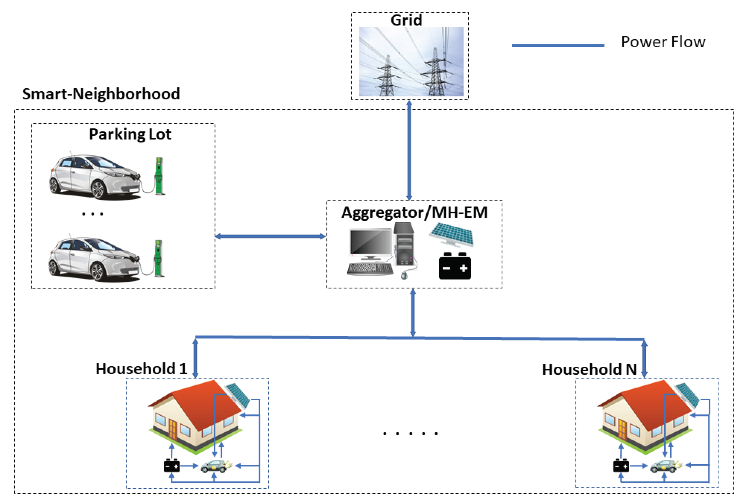

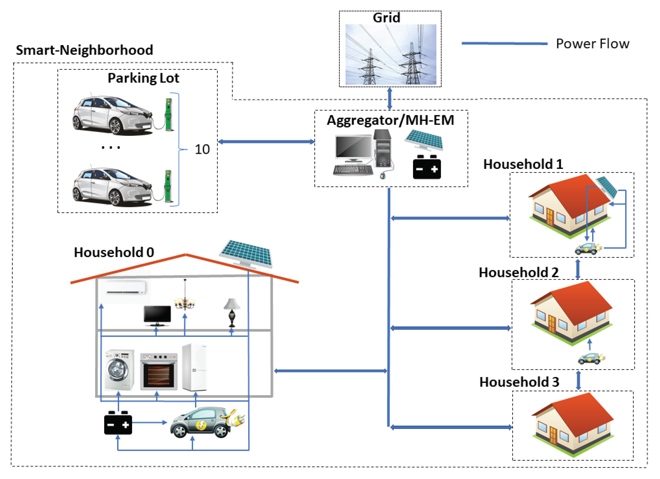


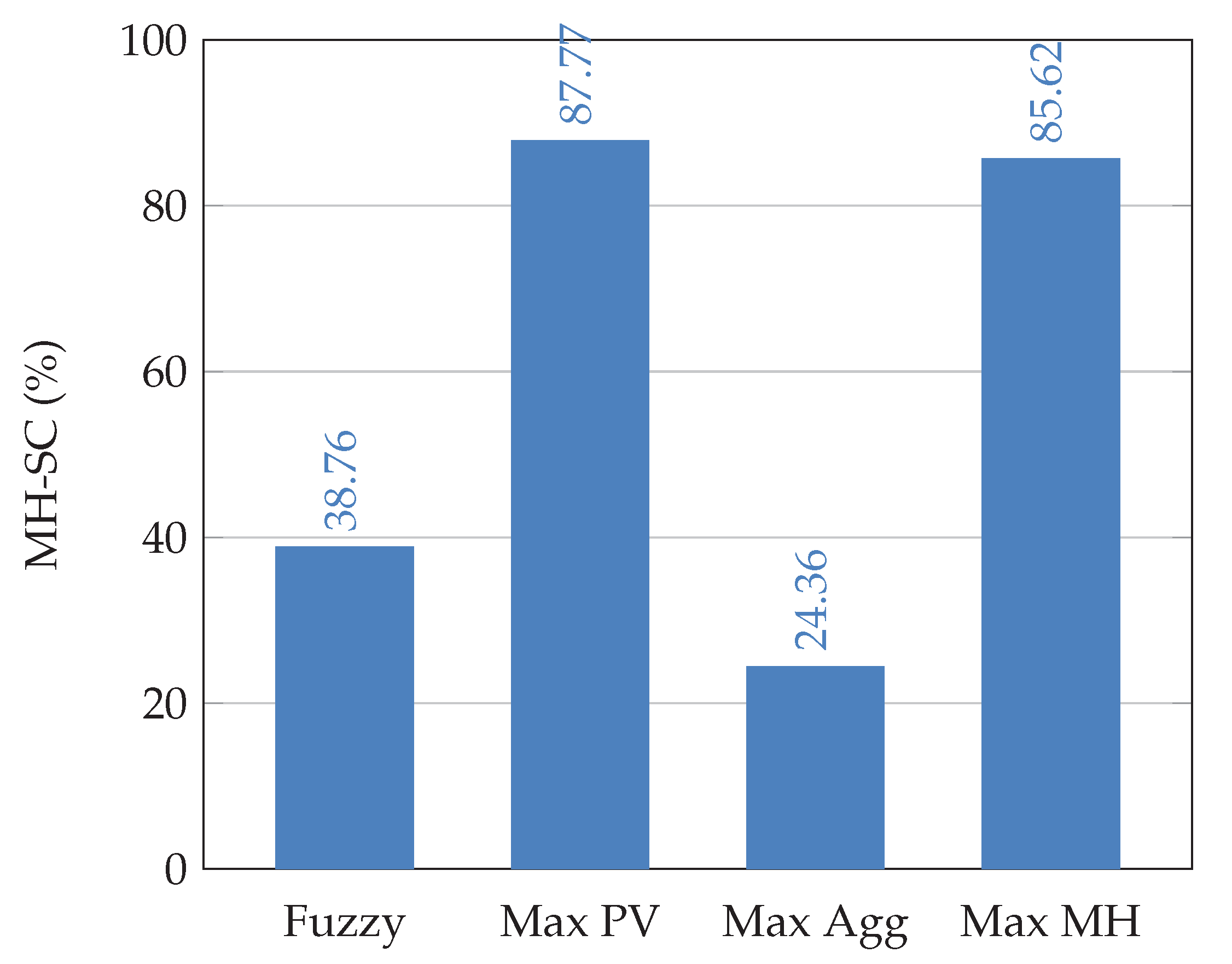

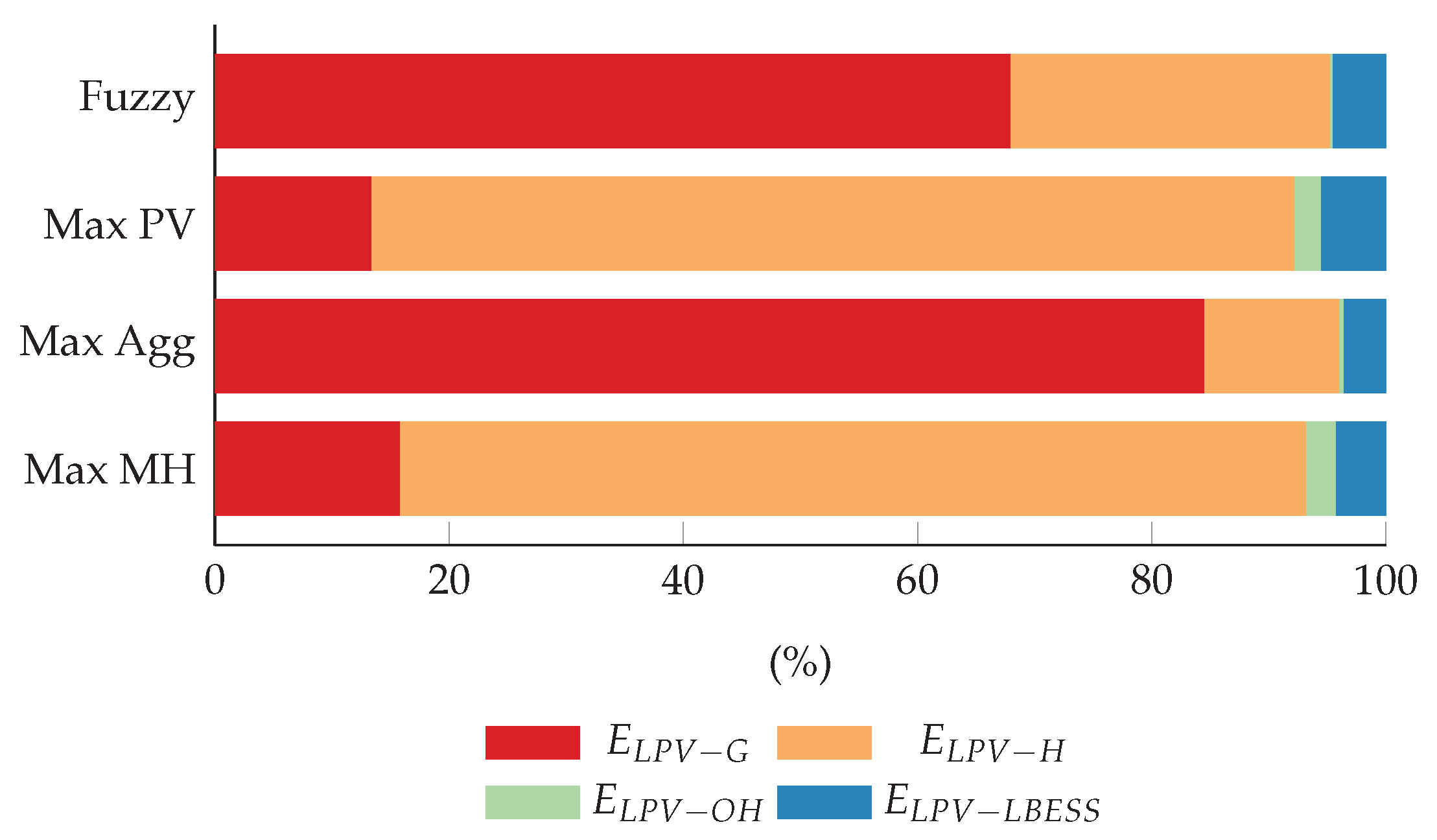

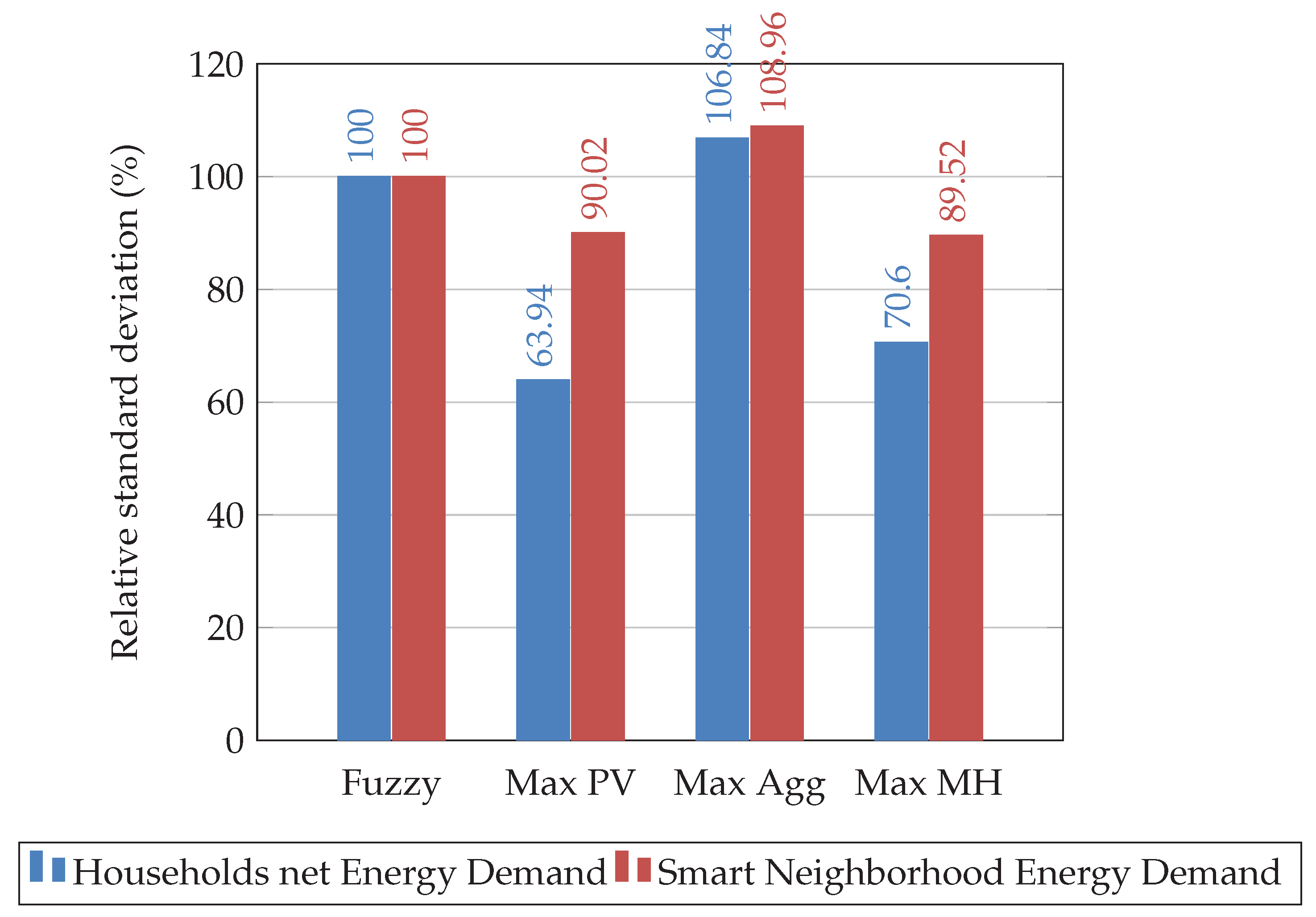
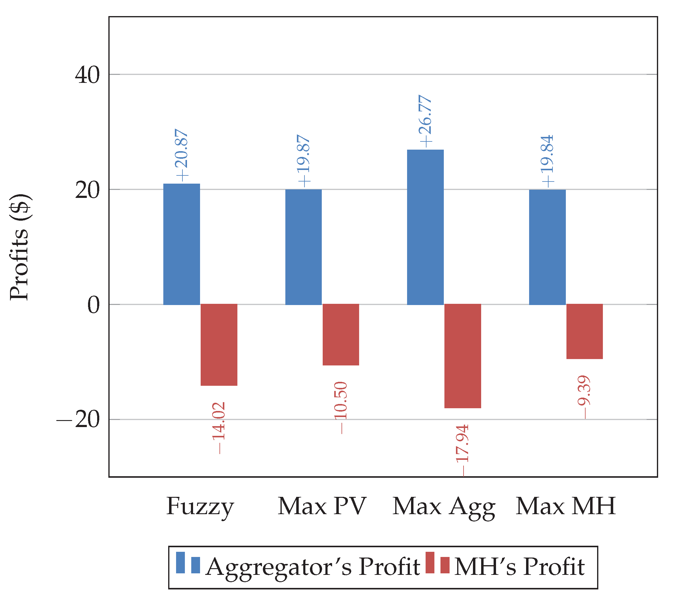

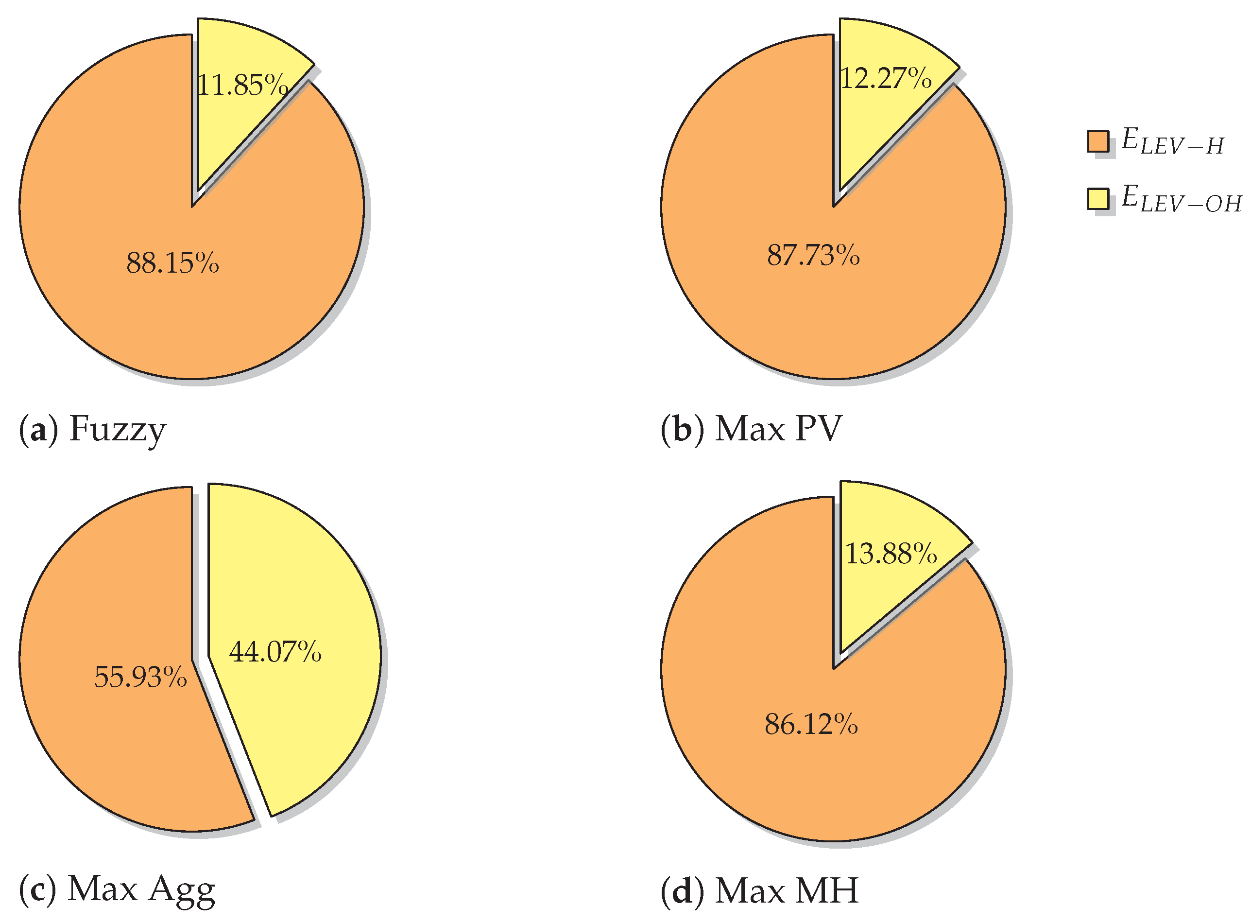