Abstract
Deep learning methods are currently used in industries to improve the efficiency and quality of the product. Detecting defects on printed circuit boards (PCBs) is a challenging task and is usually solved by automated visual inspection, automated optical inspection, manual inspection, and supervised learning methods, such as you only look once (YOLO) of tiny YOLO, YOLOv2, YOLOv3, YOLOv4, and YOLOv5. Previously described methods for defect detection in PCBs require large numbers of labeled images, which is computationally expensive in training and requires a great deal of human effort to label the data. This paper introduces a new unsupervised learning method for the detection of defects in PCB using student–teacher feature pyramid matching as a pre-trained image classification model used to learn the distribution of images without anomalies. Hence, we extracted the knowledge into a student network which had same architecture as the teacher network. This one-step transfer retains key clues as much as possible. In addition, we incorporated a multi-scale feature matching strategy into the framework. A mixture of multi-level knowledge from the features pyramid passes through a better supervision, known as hierarchical feature alignment, which allows the student network to receive it, thereby allowing for the detection of various sizes of anomalies. A scoring function reflects the probability of the occurrence of anomalies. This framework helped us to achieve accurate anomaly detection. Apart from accuracy, its inference speed also reached around 100 frames per second.
1. Introduction
Printed circuit boards (PCBs) are the most crucial and basic components for any electronic device or gadget. PCB industries are playing a vital role in the development of electronics industries. As witnessed, this world is highly dependent on electronics, and industries that produce electronics products need to ensure that those products are perfect and there should not be any defects. PCBs are a combination of laminated materials, fiberglass, or composite epoxy as solid thin plates, finally used as a base that supports electronic components [1,2,3,4]. They are designed in such a way that different electronic devices and chips can be mounted on the PCBs.
PCBs are the basic and most essential component of any electronic product that need to be designed, manufactured, and inspected accurately. There are many automated testing machines, such as automated visual inspection (AVI) and automated optical inspection (AOI) machines, for inspecting the final PCB product. Recently, the demands of the modern manufacturing process have been geared up and therefore the PCB inspection process has been improved. Recent research has proven that deep learning and computer vision techniques have been outperforming the traditional PCB defect detection technique [5,6,7]. In conventional or traditional techniques, the initial classification is performed by an AOI machine and then a quality inspection engineer verifies and confirms the classification. Even after using machines, such as AOI and AVI, for quality inspection, there are still some defects that cannot be detected using these traditional methods [8,9,10,11,12], which eventually leads to a defective PCB being delivered to the customer and used in the production of electronic gadgets, such as like televisions, watches, and phones [8]. A malfunction or any accident due to defective PCB could lead to a dangerous situation. Apart from commercial products, PCBs are also used in defense sectors, such as global positioning system (GPS) navigation systems for fighter jets and rocket launching systems, and a small error due to a faulty PCB could lead to a catastrophic situation.
In previous studies, researchers have used many effective methods to detect the defects in PCBs [13,14,15,16], such as you only look once (YOLO) of tiny YOLO, YOLOv2, YOLOv3, YOLOv4, and YOLOv5, with several different backbones, such as ResNet, RetinaNet, AlexNet, VGGNet, and GoogLeNet [17,18,19,20], and reported impressive and accurate results. Such methods are appreciated and even accepted by many industries and are used in daily quality inspection. In contrast to their good performance, there are many drawbacks to the above methods, for example, they need a large amount of data. In our past research, we used almost 20,000 images from training, which is an extensive and time-consuming process. Image collection not only takes a great deal of time, but trained manpower is also required for labelling. This research proposes a powerful and simple approach to this issue. Anomaly detection is simply defined as input images which are different from normal images, also known as abnormal images, and identification of such different patterns has shown advancement in video surveillance [21,22], product quality control [23,24,25], and medical diagnosis [26,27,28].The basic and most important reason to use anomaly detection is the challenge of different and inconsistent types of anomaly data, which are very difficult to collect and use for training in the supervised learning method.
Anomaly detection is the process of identifying outliers that have unexpected patterns with respect to normal data distribution. It has been applied in various fields, such as cybersecurity [29,30], optical inspection in manufacturing [31,32,33,34], and for medical applications [27,35]. Compared to conventional rule-based or supervised solutions, unsupervised anomaly detection approaches train models based on only normal samples, which work more logically because they do not require any prior information about anomalies before seeing the defects. This is very important for real-world applications, such as manufacturing inspection, where it is difficult to collect sufficient defective samples before detection.
Anomaly detection is more suitable as an unsupervised learning problem to solve, because the abnormal situation, in reality, is simply unpredictable and there is no label to use. For a typical industrial business scenario, such as PCB production, normal and qualified PCB samples are easy to obtain. However, in actual production, the PCB has abnormal defects known as anomalies. The type, size, location, and shape of these anomalies are very random, and are impossible to label and abstract into a supervised classification problem to solve. When solving such problems, to be as practical as possible, only normal sample information can be used.
Fundamentally, in anomaly detection there are two types of methods used: image-level anomaly detection and pixel anomaly detection. Image-level techniques manifest anomalies in the form of images of an unseen category. These methods can be coarsely divided into three branches: reconstruction-based, distribution-based, and classification-based. Pixel-level techniques are designed particularly for visual anomaly detection. Both these methods aim to precisely segment the anomalous regions in the test images. This task is much more complicated than a binary classification.
This paper describes the effectiveness of anomaly detection, followed by the student–teacher framework with its advantages of improving accuracy and efficiency. As a teacher on image classification, a strong pre-trained model was defined to learn the distribution of anomaly-free images, from which we filtered the knowledge into a student network with a similar architecture; this one-step transfer conserves the pivotal clues as much as possible. A mixture of multi-level knowledge from the features pyramid goes through a better supervision, known as hierarchical feature alignment, which allows the student network to receive it, thereby allowing the detection of various sizes of anomalies. The distinction between feature pyramids generated by both networks serves as a scoring function that stipulates the probability of an anomaly occurring. Almost 3000 images were used for training that were collected in the form of a single golden sample PCB that was 20,000 × 20,000 pixels in size. The 3000 images were equally mapped to a size of 250 × 250 pixels and extracted from the panel. Previous work was compared with the current research, from which benefits emerged in three directions. Initially, feature learning was customized to the training dataset, which made the student network discerning. Second, using a one-step transfer method, the important features were transferred from the pre-trained network to the student network, as they share an identical structure. Finally, the proposed feature pyramid matching strategy of scale invariance was facilely outstretched. Such characteristics led our framework and algorithm to achieve accuracy and fast pixel-level anomaly detection.
2. Materials and Methods
2.1. PCB Data Set
In this study, 3000 images were collected for the experiment. A single PCB panel is referred to as a golden sample. The PCB had two sides and each side was 20,000 × 20,000 pixels thus, we extracted each section of PCB by dividing it into 3000 sections, where each section was 250 × 250 pixels. These 3000 images covered almost every section and region of the PCB.
2.2. Method
2.2.1. Framework
The student–teacher learning framework was implemented to design the feature dispensation of the normal training images, as shown in Figure 1. The teacher is an influential network which is pre-trained on image classification tasks (ImageNet is trained on ResNet18). The student structure is an identical network that eventually decreases the information loss. This is in essence one case of feature-based knowledge distillation [36]. The position of the selected filtration feature has to be considered as a key factor. For each input image, a pyramid of features is generated by deep neural networks via encoding of low-level information, such as color, edge, and texture, which represents the higher-resolution features from the bottom layers. Usually, ResNet results are formatted in pyramid. The earlier layers of this pyramid result in higher resolution features encoding less context. Later layers encode lower resolution features, which encodes more context and features but at a lower spatial resolution. These layers contain both fine-grained local features and global context. To perform effective alignment, we described each location using features from the different levels of the feature pyramid.
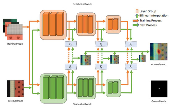
Figure 1.
Schematic overview of student–teacher feature pyramid framework.
Alignment by dense correspondences is an effective way of determining the parts of an image that are normal vs. those that are anomalous. In order to perform the alignment effectively, it is necessary to determine the features for matching. Since the proposed method uses features from a pre-trained deep ResNet CNN, the ResNet results were formatted in a pyramid to present the features. Similar to image pyramids, earlier layers result in higher resolution features encoding less context. Later layers encode lower resolution features, which encode more context but at a lower spatial resolution. To perform effective alignment, we described each location using features from the different levels of the feature pyramid. Specifically, features from the output of the last blocks were of special interest. These features encode both fine-grained local features and global context. This allowed us to find correspondences between the target image and normal images, rather than having to explicitly align the images, which is more technically challenging and brittle. The proposed method is scalable and easy to deploy in practice.
Initially, low-resolution features that have context information are yielded by top layers. Most of the important features are generated by bottom layers of the model, which are collective and can be shared through a different vision task [37]. Additionally, the distinct receptive fields are corresponded from disparate layers in the deep neural network. These are the features from the bottom layers that are extracted from teachers to guide the student network. Finally, anomalies of various sizes are detected through the hierarchical feature matching of the network.
2.2.2. Training Process
A group of anomaly-free images is the training data , ,… }, and its purpose is to extract the normal data manifold, so the L bottom layer groups are aligned with the student. is an input image, in which w is denoted as width, h is denoted as height, and c is denoted as color channels. A feature map is generated from the lth bottom layers group of the student and teacher, which is and , respectively, where and are considered as the width and height of the feature map, respectively. Although there was no preceding reference regarding the appearance of objects, we considered only anomaly free images for training. In the feature maps from the student and teacher, respectively, it should be noted that and are the most important feature vectors at position (i, j) .-the distance between the -normalized feature vectors, is characterized as a loss at position (I, j).
It is worth mentioning that the distance in Equation (1) is equivalent to the cosine similarity. Equation (1) considers cosine similarity because the loss is defined as the difference between the predicted and true label, which is quite similar to cosine similarity, i.e., L2 loss function = . The hidden vector represents for the token for the teacher and student. We were interested in a loss function that considered the probability distribution as a whole and not point-wise errors. The L2 loss function used to minimize the error is the sum of the all the squared differences between the true value and the predicted value. This is the reason loss ∊ (0, 1). An average of the loss at each position is the loss for the entire image .
In anomaly detection, where represents the impact of the lth feature scale on anomaly detection, this lth feature scale is extracted from lth bottom layer of each block of network. In all our experiments, the parameters were denoted as = 1, = 1, . . . , L. From the training data set D, a mini batch B is sampled. Using the stochastic optimization algorithm, we updated the student by minimizing the loss . Essentially, the feature map is generated from the features extracted by the last layers of different blocks. It consists of different features depending on what kind of filters and padding are used during convolution. For example, in the first block edge, filters are used that extract the feature vectors of edge in the image. Fundamentally, feature vectors are the feature of the particular layer in the block. The teacher is stable and constant during the entire training process.
2.2.3. Test Process
In this section, a test image J ∈ or goal is assigned by an anomaly map Ω with size. The deviation of pixel position (,) from the training data manifold is indicated by score . Test image J is forwarded into the student and teacher networks. and denote the feature maps that are generated by the th bottom layer group of the student and teacher, respectively. An anomaly map ) of size ×, is calculated, in which element is the loss (1) at position (,). With the help of the bilinear interpolation technique, the anomaly map is upsampled using Equation (4) to size × . The element-wise production of these interpolations is defined by the final anomaly map as:
The anomaly score is directly based on Equation (4) during the testing process where the testing image is forwarded with the aim to assign it to an anomaly map. The image is forwarded to both student and teacher during testing. The feature map generated by both networks is compared and anomaly map is generated. The anomaly map is upsampled using bilinear interpolation, which is a resampling method that uses the distance weighted average of the four nearest pixel values to estimate a new pixel value. The four cell centers from the input raster are closest to the cell center for the output processing cell, which is weighted based on distance and then averaged. The anomalous region in the image during testing is marked as anomaly. Therefore, the anomaly score for the test image J has a maximum value in the anomaly map of max (Ω).
3. Results
In order to achieve better performance, NVidia TITAN-V GPU was used with the framework using the PyTorch library, which eventually accelerated the inference speed. After discussing the structure, the training process is explained below. First, the teacher model was pre-trained on ImageNet, and then the teacher model and the student model together underwent distillation learning training. During distillation learning training, the sliding window mechanism is used to divide the picture into patches, and the same patch is sent to the teacher and each student model at the same time. Finally, the output of the student model was used to approximate the output of the teacher model to complete the distillation of this knowledge. In this anomaly detection, both image-level and pixel-level was introduced and implemented. To implement this method, we initiated this experiment with 3000 good images of PCB and selected the first three blocks of ResNet18 as the pyramid feature extractors (i.e., conv2 x, conv3 x, and conv4 x). Values from the pre-trained ResNet18, which was trained on ImageNet, were taken as parameters of the teacher network, and the student network was randomly initialized. Initially, stochastic gradient descent (SGD) was used as an optimizer and was iterated 500 times with a learning rate of 0.4. The batch size and weight decay were 32 and 10−4, respectively. Following the first experiment, a second experiment was performed using an Adam optimizer. To strike a balance between detection efficiency and accuracy, the images in the datasets were reshaped to 256 × 256. In total, almost 215 images were used for testing.
A total of 10 cross-validations were implemented for the evaluation of the models [38]. Here, the data is divided into 10 equally distributed segments, where nine of them are used for training and the remaining one is used for testing. After the training process, the model is tested on the remaining data segment, repeating the process for the same model 10 times by reshuffling the data and performing the training and testing. A new dataset is used for testing every time so the model does not repeat the same data for testing. As mentioned previously, two types of experiments were conducted. The first experiment used SGD optimizers with a learning rate of 0.04 and 10 cross-validations using the same hyper parameters, which was followed by the second experiment in which a change was introduced (i.e., changing the SGD optimizers to Adam optimizers and the learning rate to 0.001). Table 1 displays the confusion matrix for both experiments. In total, there are 20 cross-validations which display the representative true positives, false negatives, false positives, and true negatives. The cells are labeled as OK or NG.

Table 1.
Confusion matrix of ten different cross-validations for SGD optimizers with learning rate 0.04 and Adam optimizers with learning rate 0.001.
In Table 2, STPM (student–teacher feature pyramid matching) shows anomaly detection for the first experiment, in which the hyper parameters were set to SGD optimizer with a learning rate of 0.04. In the table, the false positive rate, precision, accuracy, true positive rate, prevalence, and misclassification for all the 10 cross-validations are shown, in addition to the standard deviation of accuracy and the mean.
Table 2.
Misclassification rate, accuracy, false positive rate, true negative rate, true positive rate, prevalence, precision, standard deviation of accuracy, and mean.
Table 3 shows the misclassification rate, accuracy, false positive rate, true negative rate, true positive rate, prevalence, precision, standard deviation of accuracy, and mean for 10 cross-validations. In this section of the experiment, the hyper parameters were changed to Adam optimizers and the learning rate was reduced from 0.04 to 0.001, which eventually increased the accuracy of the model.
Table 3.
Misclassification rate, accuracy, false positive rate, true negative rate, true positive rate, prevalence, precision, standard deviation of accuracy, and mean.
Figure 2 shows true positive images, which consist of a defective region and were predicted as NG, in which the heat map and classification are shown with segmentation where the defective region has been classified. Figure 3 displays false negative images, which are actually defective images that were predicted as good or normal images, which do not represent any defective region. Figure 4 displays sample images of a true negative class, which do not consist of any defective regions, and using our model were classified as good or anomaly-free images. Finally, Figure 5 displays the false positive class in which a defective region has been segmented and displayed in the image; however, there is no defects in these images. Its classification and segmentation are wrong, and that is the reason it is known as a false positive.
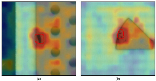
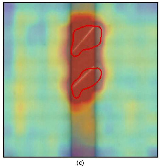
Figure 2.
True positive PCB example. (a) True positive example 1; (b) True positive example 2; (c) True positive example 3.
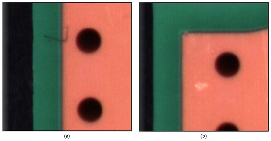
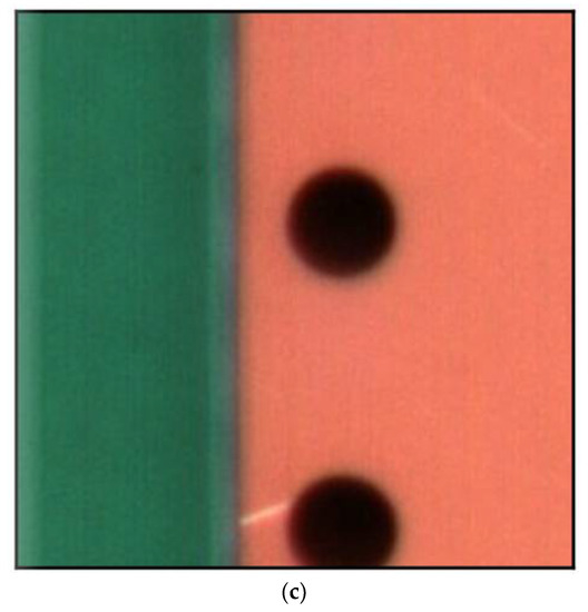
Figure 3.
False negative PCB example. (a) False negative example 1; (b) False negative example 2; (c) False negative example 3.
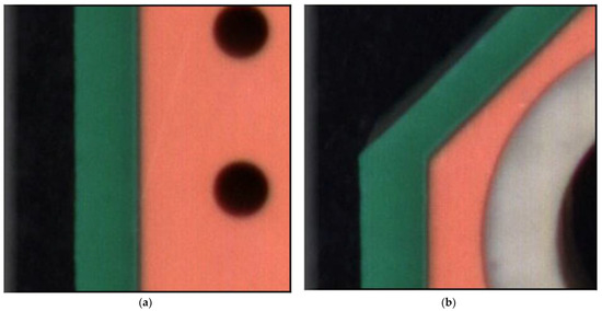
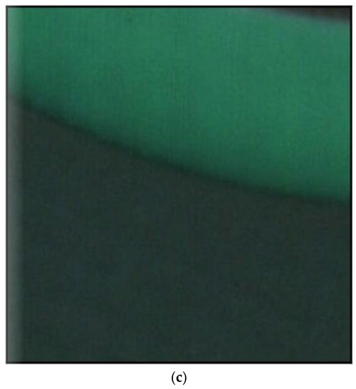
Figure 4.
True negative PCB example. (a) True negative example 1; (b) True negative example 2; (c) True negative example 3.
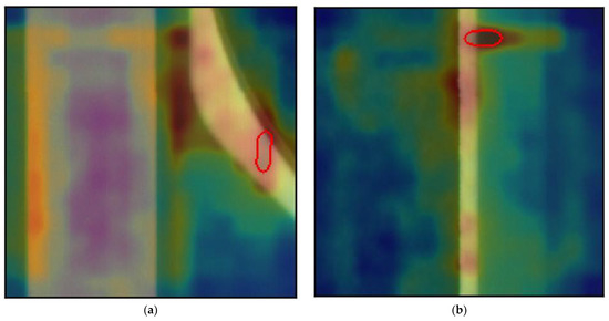
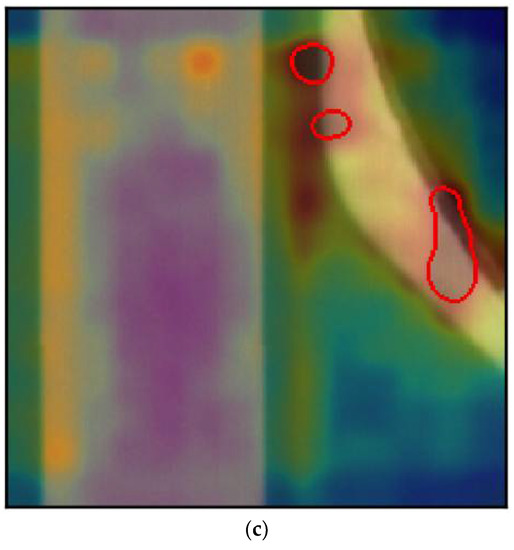
Figure 5.
False positive of PCB section. (a) False positive example 1; (b) False positive example 2; (c) False positive example 3.
It can be seen that unsupervised learning can also be used in industries and in real time scenarios, as its accuracy is acceptable and competitive with the previously implemented yolo-v5 model. It is also better in other aspects, such as computing training time and memory. In Table 4 below, the difference of memory and training time used by both the supervised and unsupervised method is displayed.
Table 4.
Comparing time and memory for Yolov5-Large and Anomaly Detection-STPM.
4. Discussion
Anomaly detection for defects in PCB leads to the development of the-state-of-the-art algorithms that can be implemented to enhance the quality of the inspection process. In this process, only 3000 images were used, which is 86% less than in the previous methods. Unsupervised learning reduces the data pre-processing (i.e., labeling the image), where many skilled quality engineers have traditionally been dedicated to this work. The introduction of anomaly detection is a game changing method that is more powerful and faster than other supervised learning methods [38,39,40]. A pre-trained ResNet-18 was used in this research to accelerate the inference speed, because it is faster and more compact than other backbone algorithms, such as ResNet34, ResNet50, ResNet101, and ResNet152.
Unsupervised methods have been utilized as there are major drawbacks to supervised learning. In the unsupervised learning method, non-labeled data is used for the machine to learn patterns and automatically inherit characteristics with automatic classification [41]. During inference, when new data passes through, the machine predicts and classifies which class it belongs to. Meaningful vectors describing the entire image are extracted through deep neural networks, and the distance between the vectors of the test images and the reference vector representing normality from the training dataset is considered as the anomaly score.
Anomaly detection is an unsupervised learning that deals with the sudden occurrence of anomalies. This paper’s goal was to develop a simple and powerful method to solve this problem. The research was initiated using a student–teacher framework because it has substantially expanded in terms of its efficiency and accuracy. The teacher is used as pre-trained image classification model, and knowledge is extracted into a student network with the same architecture to learn the distribution of images without anomalies. A mixture of multi-level knowledge from the features pyramid passes through a better supervision, known as hierarchical feature alignment, which allows the student network to receive it, thereby allowing the detection of various sizes of anomalies. A scoring function reflects the probability of the occurrence of anomalies, and is described as the difference between the features pyramids generated by the two networks. Such operations lead to more accurate and faster pixel-level anomaly detection.
As shown in Table 2, when SGD was used for optimization and and the hyper parameter learning rate was set 0.04, the mean and standard deviation of accuracy were 94.63 ± 0.68, and the highest accuracy between the 10 cross-validations were cross-validation 4 and cross-validation 7, which were both 95.34%. Later, the hyper parameters were tuned to switch to Adam optimizers and reduce the learning rate to 0.001, which eventually increased the mean and standard deviation of accuracy to 97.43 ± 0.52, and the highest accuracy between the 10 cross-validations was cross-validation 5 (98.15%), as shown in Table 3. It can be observed that reducing the learning rate plays an important role in reducing the loss and increasing the accuracy, which eventually reaches the global minima.
The most important and encouraging reason to endorse this method is that it achieved an overall average accuracy of 97.43% with a standard deviation of 0.52. Apart from its accuracy, this method reduces the time of pre-processing through bypassing the labeling section. Finally, it can be seen in Table 2 and Table 3 that defects in PCB are detected with impressive accuracy and precision using this method.
5. Conclusions
Defect detection in PCB is a crucial move for industry 4.0. Research on PCB defect detection is an essential step towards the application of deep learning methods in industry. This article is a step towards application of unsupervised learning, which uses less data compared to supervised learning, which can transform the application of computers in industry.
This study showed that anomaly detection with a STPM framework achieved an accuracy of 97.43%. Hence, our future goals are to improve accuracy and inference using anomaly detection and potentially to conduct the experiment using meta learning. Aside from the STPM framework, further work is required to increase accuracy and to classify and detect several other kinds of defects by implementing and introducing algorithms and frameworks, such as SPADE [42], PaDIM, PatchCore [43], etc. In addition, self-organizing maps and deep belief networks might also be used for PCB defect detection.
Author Contributions
Conceptualization V.A.A., Y.-C.H., A.U., H.-C.C., M.F.A. and J.-S.S.; formal analysis, V.A.A., Y.-C.H., and J.-S.S.; investigation, V.A.A., Y.-C.H. and J.-S.S.; methodology, V.A.A., Y.-C.H. and J.-S.S.; software, V.A.A., Y.-C.H. and J.-S.S.; supervision, V.A.A., Y.-C.H., M.-C.C., H.-C.K., M.F.A. and J.-S.S.; validation, V.A.A., Y.-C.H., M.F.A. and J.-S.S.; visualization, V.A.A., Y.-C.H., H.-C.C. and J.-S.S.; writing, V.A.A., Y.-C.H., M.F.A. and J.-S.S. All authors have read and agreed to the published version of the manuscript.
Funding
This research was funded by the Ministry of Science and Technology (MOST) of Taiwan (grant number: MOST 109-2622-E-155-007), Avary Holding (Shenzhen) Co., Ltd and Boardtek Electronics Corporation, Taiwan.
Conflicts of Interest
The authors declare no conflict of interest.
References
- Suzuki, H. Junkosha Co Ltd. Official Gazette of the United States Patent and Trademark. Printed Circuit Board. U.S. Patent 4,640,866, 16 March 1987. [Google Scholar]
- Matsubara, H.; Itai, M.; Kimura, K. NGK Spark Plug Co Ltd. Patents Assigned to NGK Spark Plug. Printed Circuit Board. U.S. Patent 6,573,458, 12 September 2003. [Google Scholar]
- Magera, J.A.; Dunn, G.J. Motorola Solutions Inc. The Printed Circuit Designer’s Guide to Flex and Rigid-Flex Fundamentals. Printed Circuit Board. U.S. Patent 7,459,202, 21 August 2008. [Google Scholar]
- Cho, H.S.; Yoo, J.G.; Kim, J.S.; Kim, S.H. Samsung Electro Mechanics Co Ltd. Official Gazette of the United States Patent and Trademark. Printed Circuit Board. U.S. Patent 8,159,824, 16 March 2012. [Google Scholar]
- Chauhan, A.P.S.; Bhardwaj, S.C. Detection of bare PCB defects by image subtraction method using machine vision. In Proceedings of the World Congress on Engineering, London, UK, 6–8 July 2011; Volume 2, pp. 6–8. [Google Scholar]
- Khalid, N.K.; Ibrahim, Z. An Image Processing Approach towards Classification of Defects on Printed Circuit Board. Ph.D. Thesis, Universiti Teknologi Malaysia, Johor, Malaysia, 2007. [Google Scholar]
- Bengio, Y.; Courville, A.; Vincent, P. Representation Learning: A Review and New Perspectives. IEEE Trans. Pattern Anal. Mach. Intell. 2013, 35, 1798–1828. [Google Scholar] [CrossRef] [PubMed]
- Malge, P.S. PCB Defect Detection, Classification and Localization using Mathematical Morphology and Image Processing Tools. Int. J. Comput. Appl. 2014, 87, 40–45. [Google Scholar]
- Takada, Y.; Shiina, T.; Usami, H.; Iwahori, Y. Defect Detection and Classification of Electronic Circuit Boards Using Keypoint Extraction and CNN Features. In Proceedings of the Ninth International Conferences on Pervasive Patterns and Applications Defect, Athens, Greece, 19–23 February 2017; pp. 113–116. [Google Scholar]
- Anitha, D.B.; Mahesh, R. A Survey on Defect Detection in Bare PCB and Assembled PCB using Image Processing Techniques. In Proceedings of the 2017 International Conference on Wireless Communications, Signal Processing and Networking (WiSPNET), Chennai, India, 22–24 March 2017; pp. 39–43. [Google Scholar]
- Crispin, A.J.; Rankov, V. Automated inspection of PCB components using a genetic algorithm template-matching approach. Int. J. Adv. Manuf. Technol. 2007, 35, 293–300. [Google Scholar] [CrossRef] [Green Version]
- Raihan, F.; Ce, W. PCB Defect Detection USING OPENCV with Image Subtraction Method. In Proceedings of the 2017 International Conference on Information Management and Technology (ICIMTech), Singapore, 27–29 December 2017; pp. 204–209. [Google Scholar]
- Hosseini, H.; Xiao, B.; Jaiswal, M.; Poovendran, R. On the Limitation of Convolutional Neural Networks in Recognizing Negative Images. In Proceedings of the 2017 16th IEEE International Conference on Machine Learning and Applications (ICMLA), Cancun, Mexico, 18–21 December 2017; pp. 352–358. [Google Scholar]
- Tao, X.; Wang, Z.; Zhang, Z.; Zhang, D.; Xu, D.; Gong, X.; Zhang, L. Wire Defect Recognition of Spring-Wire Socket Using Multitask Convolutional Neural Networks. IEEE Trans. Compon. Packag. Manuf. Technol. 2018, 8, 689–698. [Google Scholar] [CrossRef]
- Uijlings, J.R.R.; Van De Sande, K.E.A.; Gevers, T.; Smeulders, A.W.M. Selective Search for Object Recognition. Int. J. Comput. Vis. 2012, 104, 154–171. [Google Scholar] [CrossRef] [Green Version]
- Girshick, R.; Donahue, J.; Darrell, T.; Malik, J. Rich feature hierarchies for accurate object detection and semantic segmentation. In Proceedings of the 2014 IEEE Conference on Computer Vision and Pattern Recognition, Columbus, OH, USA, 23–28 June 2014; pp. 580–587. [Google Scholar]
- He, K.; Zhang, X.; Ren, S.; Sun, J. Deep residual learning for image recognition. arXiv 2015, arXiv:1512.03385. [Google Scholar]
- Simonyan, K.; Zisserman, A. Very deep convolutional networks for large-scale image recognition. arXiv 2014, arXiv:1409.1556. [Google Scholar]
- Szegedy, C.; Ioffe, S.; Vanhoucke, V. Inception-v4, inception-resnet and the impact of residual connections on learning. arXiv 2016, arXiv:1602.07261. [Google Scholar]
- Szegedy, C.; Liu, W.; Jia, Y.; Sermanet, P.; Reed, S.; Anguelov, D.; Erhan, D.; Vanhoucke, V.; Rabinovich, A. Going deeper with convolutions. arXiv 2014, arXiv:1409.4842. [Google Scholar]
- Abati, D.; Porrello, A.; Calderara, S.; Cucchiara, R. Latent space autoregression for novelty detection. In Proceedings of the IEEE/CVF Conference on Computer Vision and Pattern Recognition, Long Beach, CA, USA, 16–20 June 2019. [Google Scholar]
- Roitberg, A.; Al-Halah, Z.; Stiefelhagen, R. Informed democracy: Voting-based novelty detection for action recognition. In Proceedings of the 29th British Machine Vision Conference, Newcastle, UK, 3–6 September 2018. [Google Scholar]
- Bergmann, P.; Fauser, M.; Sattlegger, D.; Steger, C. Mvtec AD—A comprehensive real-world dataset for unsupervised anomaly detection. In Proceedings of the IEEE/CVF Conference on Computer Vision and Pattern Recognition, Long Beach, CA, USA, 16–20 June 2019. [Google Scholar]
- Bergmann, P.; Fauser, M.; Sattlegger, D.; Steger, C. Uninformed students: Student-teacher anomaly detection with discriminative latent embeddings. In Proceedings of the IEEE/CVF Conference on Computer Vision and Pattern Recognition, Seattle, WA, USA, 13–19 June 2020. [Google Scholar]
- Napoletano, P.; Piccoli, F.; Schettini, R. Anomaly detection in nanofibrous materials by CNN-based self-similarity. Sensors 2018, 18, 209. [Google Scholar] [CrossRef] [Green Version]
- Schlegl, T.; Seebock, P.; Waldstein, S.M.; Langs, G.; Schmidt-Erfurth, U. f-AnoGAN: Fast unsupervised anomaly detection with generative adversarial networks. Med. Image Anal. 2019, 54, 30–44. [Google Scholar] [CrossRef]
- Schlegl, T.; Seebock, P.; Waldstein, S.M.; Schmidt-Erfurth, U.; Langs, G. Unsupervised anomaly detection with generative adversarial networks to guide marker discovery. In Proceedings of the International Conference on Information Processing in Medical Imaging, Boone, NC, USA, 25–30 June 2017. [Google Scholar]
- Vasilev, A.; Golkov, V.; Lipp, I.; Sgarlata, E.; Tomassini, V.; Jones, D.K.; Cremers, D. q-Space novelty detection with variational autoencoders. arXiv 2018, arXiv:1806.02997. [Google Scholar]
- Ayush, H.; Ankit, G.; Trisha, P. CAMLPAD: Cybersecurity autonomous machine learning platform for anomaly detection. In Advances in Information and Communication; Springer: Cham, Switzerland, 2020; pp. 705–720. [Google Scholar]
- Ibrahim, A.; Ali, A.; Esam, A.; Raed, A.; Mohamed, Z.; Hua, M. Ad-IoT: Anomaly detection of IoT cyberattacks in smart city using machine learning. In Proceedings of the 2019 IEEE 9th Annual Computing and Communication Workshop and Conference (CCWC), Las Vegas, NV, USA, 7–9 January 2019; pp. 0305–0310. [Google Scholar]
- Hu, G.; Huang, J.; Wang, Q.; Li, J.; Xu, Z.; Huang, X. Unsupervised fabric defect detection based on a deep convolutional generative adversarial network. Text. Res. J. 2020, 90, 247–270. [Google Scholar] [CrossRef]
- Mei, S.; Yang, H.; Yin, Z. An unsupervised-learning-based approach for automated defect inspection on textured surfaces. IEEE Trans. Instrum. Meas. 2018, 67, 1266–1277. [Google Scholar] [CrossRef]
- Samet, A.; Amir, A.A.; Toby, B. GANomaly: Semi-supervised anomaly detection via adversarial training. In Asian Conference on Computer Vision, Proceedings of the 14th Asian Conference on Computer Vision, Perth, Australia, 2–6 December 2018; Springer: Cham, Switzerland, 2019; pp. 622–637. [Google Scholar]
- Zenati, H.; Foo, C.S.; Lecouat, B.; Manek, G.; Chandrasekhar, V.R. Efficient gan-based anomaly detection. arXiv 2018, arXiv:1802.06222. [Google Scholar]
- Oquab, M.; Bottou, L.; Laptev, I.; Sivic, J. Learning and transferring mid-level image representations using convolutional neural networks. In Proceedings of the IEEE Conference on Computer Vision and Pattern Recognition, Columbus, OH, USA, 23–28 June 2014. [Google Scholar]
- Wang, L.; Yoon, K.-J. Knowledge distillation and student-teacher learning for visual intelligence: A review and new outlooks. arXiv 2020, arXiv:2004.05937. [Google Scholar] [CrossRef]
- Pritt, M.; Chern, G. Satellite Image Classification with Deep Learning. In Proceedings of the 2017 IEEE Applied Imagery Pattern Recognition Workshop (AIPR), Washington, DC, USA, 10–12 October 2017. [Google Scholar]
- Zhang, X.S.; Roy, R.J.; Jensen, E.W. EEG complexity as a measure of depth of anesthesia for patients. IEEE Trans. Biomed. Eng. 2001, 48, 1424–1433. [Google Scholar] [CrossRef]
- Lalitha, V.; Eswaran, C. Automated detection of anesthetic depth levels using chaotic features with artificial neural networks. J. Med. Syst. 2007, 31, 445–452. [Google Scholar] [CrossRef]
- Peker, M.; Sen, B.; Gürüler, H. Rapid Automated Classification of Anesthetic Depth Levels using GPU Based Parallelization of Neural Networks. J. Med. Syst. 2015, 39, 18. [Google Scholar] [CrossRef]
- Dike, H.U.; Zhou, Y.; Deveerasetty, K.K.; Wu, Q. Unsupervised Learning Based on Artificial Neural Network: A Review. In Proceedings of the 2018 IEEE International Conference on Cyborg and Bionic Systems (CBS), Shenzhen, China, 25–27 October 2018; pp. 322–327. [Google Scholar]
- Defard, T.; Setkov, A.; Loesch, A.; Audigier, R. PaDiM: A Patch Distribution Modeling Framework for Anomaly Detection and Localization. arXiv 2020, arXiv:2011.08785. [Google Scholar]
- Roth, K.; Pemula, L.; Zepeda, J.; Schölkopf, B.; Brox, T.; Gehler, P. Towards Total Recall in Industrial Anomaly Detection. arXiv 2021, arXiv:2106.08265. [Google Scholar]
Publisher’s Note: MDPI stays neutral with regard to jurisdictional claims in published maps and institutional affiliations. |
© 2021 by the authors. Licensee MDPI, Basel, Switzerland. This article is an open access article distributed under the terms and conditions of the Creative Commons Attribution (CC BY) license (https://creativecommons.org/licenses/by/4.0/).