Article

Soft Robotic Sensing, Proprioception via Cable and Microfluidic Transmission

1
Department of Electrical and Computer Engineering, University of California, Santa Cruz, CA 95064, USA
2
Department of Mechanical Engineering, University of Wisconsin, Madison, Madison, WI 53706, USA
*
Author to whom correspondence should be addressed.
Electronics 2021, 10(24), 3166; https://doi.org/10.3390/electronics10243166
Submission received: 20 November 2021 / Revised: 11 December 2021 / Accepted: 16 December 2021 / Published: 19 December 2021
(This article belongs to the Special Issue Human Computer Interaction and Its Future)

Abstract

:
Current challenges in soft robotics include sensing and state awareness. Modern soft robotic systems require many more sensors than traditional robots to estimate pose and contact forces. Existing soft sensors include resistive, conductive, optical, and capacitive sensing, with each sensor requiring electronic circuitry and connection to a dedicated line to a data acquisition system, creating a rapidly increasing burden as the number of sensors increases. We demonstrate a network of fiber-based displacement sensors to measure robot state (bend, twist, elongation) and two microfluidic pressure sensors to measure overall and local pressures. These passive sensors transmit information from a soft robot to a nearby display assembly, where a digital camera records displacement and pressure data. We present a configuration in which one camera tracks 11 sensors consisting of nine fiber-based displacement sensors and two microfluidic pressure sensors, eliminating the need for an array of electronic sensors throughout the robot. Finally, we present a Cephalopod-chromatophore-inspired color cell pressure sensor. While these techniques can be used in a variety of soft robot devices, we present fiber and fluid sensing on an elastomeric finger. These techniques are widely suitable for state estimation in the soft robotics field and will allow future progress toward robust, low-cost, real-time control of soft robots. This increased state awareness is necessary for robots to interact with humans, potentially the greatest benefit of the emerging soft robotics field.

1. Introduction

Over the past decade, soft robots have shown an increasing potential to dramatically expand the capabilities of the field of robotics. Currently, however, most demonstrations have been limited to precisely that, potential. For soft robots to emerge into human-populated environments and to perform useful real-world tasks, advances are required in sensors able to quickly provide robust state information, both as individual sensors and as integrated sensing systems. Soft robots hold the potential for unprecedented levels of interaction with the surrounding environment impossible with traditional rigid-linked robots. This innate ability to yield to the environment and to sense and learn from that interaction is one of the biggest potential advantages of soft robots. By embracing this ability to interact, soft robots can fundamentally change human-robot interaction and allow safe collaboration in the home and workplace. To achieve this leap forward in state awareness and embodied intelligence, a rethinking of soft sensing is necessary.
With this novel approach to robotics and interaction come novel challenges. The number of sensors needed to understand the state of a soft robot dramatically exceed the number needed to determine the pose of a traditional rigid-link robot. Traditional robotic manipulation techniques including D-H parameters, Quaternions, and Product of Exponentials assume rigid links connected by single (often rotational or prismatic) degrees of freedom [1]. Thus, one could define the entire range of possible poses of a traditional six-link robot using only six sensors. (Additional sensors would likely be included, but for other applications such as monitoring temperature and voltage.) Arguably, defining the pose of a single soft actuator, capable of yielding to the environment and several modes of self-motion, could require more than six sensors. Traditional robots typically contact the external world via manipulators (often end-effectors), with a limited number of small contact points or contact regions, often modeled using friction cone techniques [2] requiring a single multi-axis strain gauge or even a single axis pressure sensor. Contact with components other than predefined manipulators is unusual, and unplanned contact is avoided at all costs. Some of the main advantages of soft robots are their ability to distribute forces across broad regions of an actuator and that unplanned interactions are often of minor concern. Thus, where a traditional robot may require fewer than 10 sensors to determine pose and interaction, a soft robot could easily require over a hundred. Several groups have tried machine vision methods to alleviate the rapidly growing burden of so many sensors, using cameras and motion capture to directly measure soft robot pose [3,4,5]. While this is effective in some applications, and the work is quite compelling, this technique is ill-suited to applications with a likelihood of obstructed views (such as reaching into boxes to retrieve objects in order fulfillment or laparoscopic surgery). Real-time processing of video to interpret complex 3D motions of an underactuated robot is also an extremely challenging task.
Many technologies have been presented to achieve myriad sensing modes in soft robots. Soft sensors (sensors composed of compliant materials, gels, liquids, or a combination of these housed inside a soft robotics component) have been developed using conductive grease [6], capacitive liquid [7], resistive ionic gels [8], waveguides [9], and many demonstrations with liquid metals [10,11,12], primarily focusing on a Eutectic of Gallium and Indium (EGaIn) [13]. These many sensor technologies can measure changes in length [14], bending [15], pressure [16], even temperature in the distal end of a soft finger [17]. There has been work on mixed-mode sensing models [7], including Park et al. [18], able to sense pressure and two modes of stretch, all in one sensor. Other sensing techniques used in soft robotics have involved bonding traditional bend sensors to a soft actuator [19] and embedded magnets and hall effect sensors [20]. There has been work in optical methods including the SOFTcell project by Bajcsy and Fearing [21] in which tactile response was determined through optical analysis of a deformed membrane, and video tracking of markers adhered to or embedded in soft components [5].
While these studies present compelling sensors, further development is necessary in utilizing a suite of sensors to increase overall state awareness. In both traditional and soft robotics, many have studied proprioceptive sensor systems, robot skin, and bioinspired sensing. Discussion of these broad fields can be found in reviews of various subspecialties [22,23,24,25,26]. The value of multi-sensor systems to perceive different proprioceptive or exteroceptive phenomena is widely appreciated. However, as the number of sensors is increased, the computation, data acquisition, and signal processing load drastically increase as well. Each sensor requires electronic circuitry, wiring to each sensor, and a dedicated channel to a data acquisition system or an analog to digital converter (ADC), requiring signal processing and computation. A sensor-skin with a grid of ten-by-ten sensors would be a relatively modest requirement for many perception applications. Using discrete nodes would require 100 dedicated sensors. Multiplexing by separating signals into 10 horizontal and 10 vertical sensors reduces the load to 20 separate sensors (with related disadvantages), which is still a considerable burden for a single sensor-skin device.
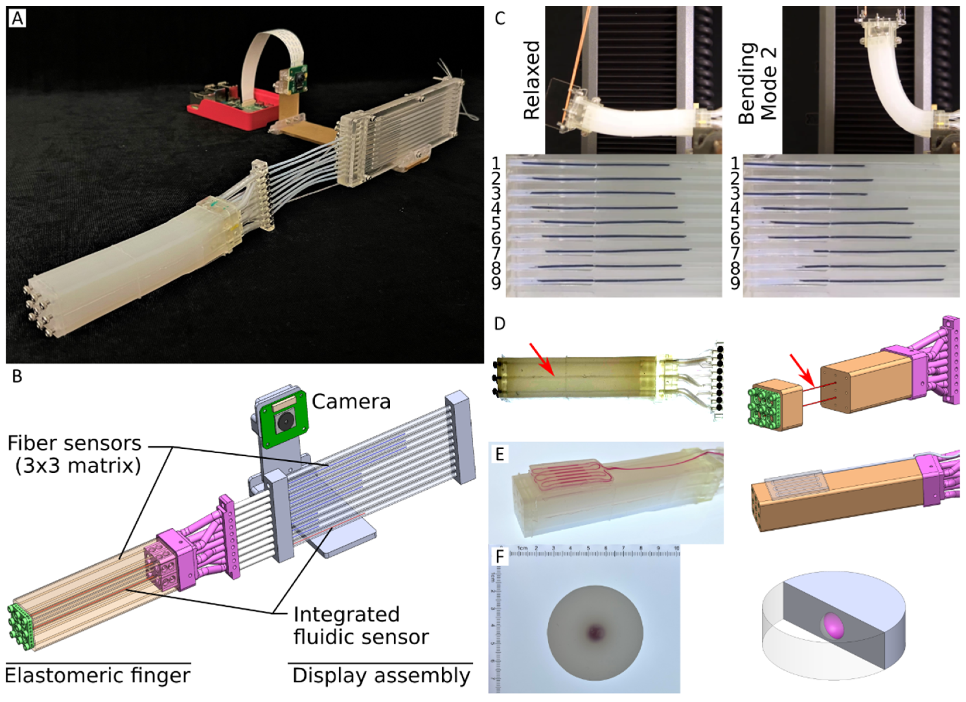
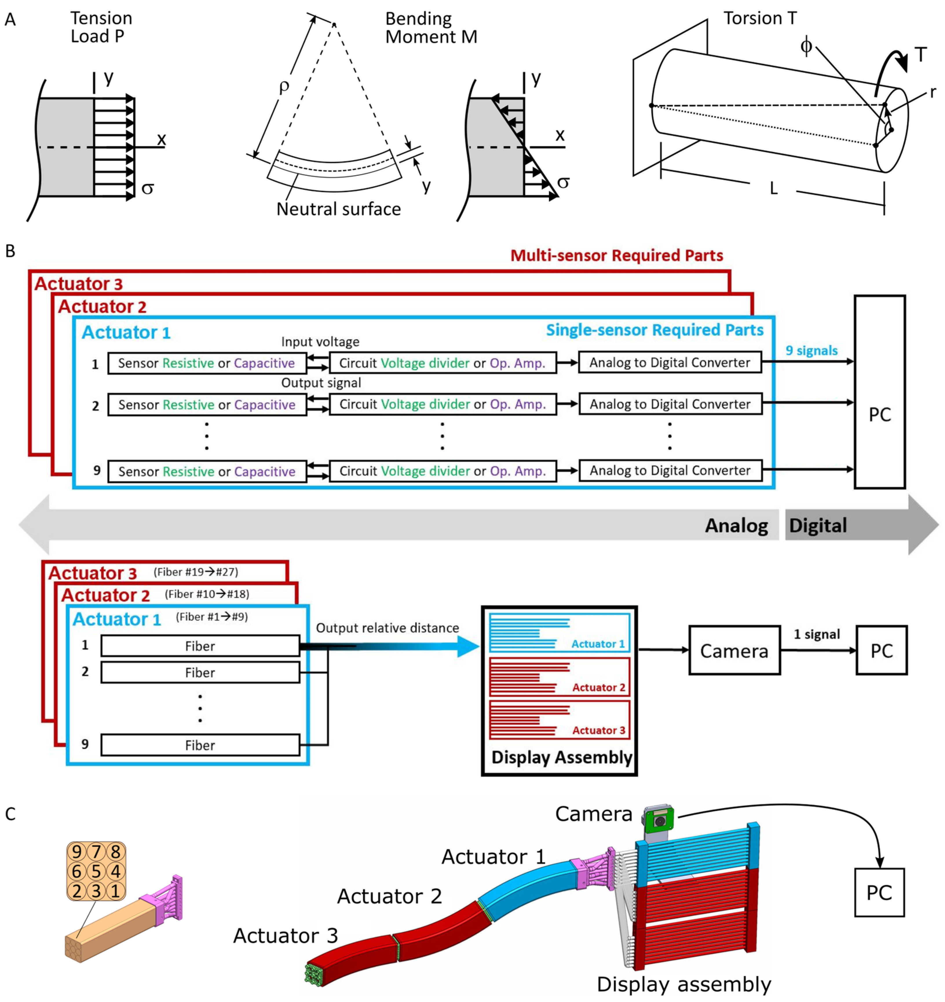
So far, soft sensors have primarily been developed as individual, standalone units. To scale the system from one to five sensors, one simply fabricates and integrates five sensors and five sets of required electronics, which interfaced to five ADCs and sent five signals to a microcontroller. The sensors in this work focus instead on passive sensors which present position and pressure data to a digital camera for real-time or offline data processing. Digital cameras, able to record multi-megapixel resolution are readily available at low cost and are already present on many robot platforms. With our method, a single camera can record and interpret data from many deformation and pressure sensors, providing a platform for state perception and embodied intelligence research. This camera does not record the elastomeric finger itself. Rather, it records the remotely located display assembly (Figure 1A,B), where it tracks the motion of fiber-based displacement sensors and microfluidic pressure sensors. Recording the sensor states rather than the elastomeric finger itself presents several advantages. Firstly, no clear line of sight is needed. During typical robotic tasks, portions of a finger would often become obstructed when environmental objects or the robot itself come between the finger and the camera. Additionally, by remotely recording the display assembly, all aspects of recording (color, contrast, lighting) can be controlled to values optimum for marker tracking, impossible in real-world robotic applications. Finally, by tracking only monochromatic markers moving in well-defined horizontal or vertical paths in a controlled environment (no unanticipated glare/obstructions), extremely simplified vision algorithms can be used, allowing much faster processing. We present three techniques in which digital cameras record markers from fiber-based deformation sensors and microfluidic pressure sensors inside an elastomeric finger-like structure. We present an elastomeric finger with embedded fiber sensors and two modes of microfluidic pressure sensor (Figure 1A,B). We present this system’s ability to quantify elongation along and twist about a longitudinal axis, and bending about the two orthogonal axes perpendicular to the longitudinal axis (Figure 1C). We also present the technique’s ability to quantify overall pressure via an integrated microfluidic sensor (Figure 1D) and local contact pressure via a surface-mounted microfluidic sensor (Figure 1E). These sensors (specifically designed to be used in groups) can be designed into soft robotic actuators, and leverage the framework provided from beam theory and classical mechanics of materials to sense the state of each actuated unit. In addition, we present a Cephalopod chromatophore-inspired color-cell pressure sensor that detects changes in local pressure through the deformation of colored liquid cells (Figure 1F). Chromatophores have been widely studied for decades [27,28,29], and in recent years have become the inspiration for biomimicry and biomimetic work by the soft robotics community [30] using bulk deformation of a matrix to modulate appearance and spell out a word [31] or disrupting part of a surface using dielectric elastomers [32]. In this work, however, we flip the concept, using the color cell as a passive pressure sensor to estimate externally applied force, not as an active device, mechanically distorted to modulate appearance.
While the simple sensor designs presented here have value individually, the key contribution of this work is that the sensors are fundamentally designed to be used in groups and leverage the concepts from beam theory and mechanics of materials to infer system state from a strategically located system of sensors. Intended to be built into a soft robot at the system level, a properly configured array of these deformation and pressure sensors can give state awareness far beyond that of individual sensors. The remainder of this paper is organized as follows: Section 2 presents the methods used, beginning with a conceptual overview and review of beam theory/mechanics of materials on which these techniques are based, followed by design and fabrication, visual algorithms, and characterization methods. Section 3 presents results, divided into fiber-based deformation sensors, microfluidic pressure sensors, and color cell pressure sensors. Section 4 presents a discussion on the work and how it relates to the field. Where relevant, sections are further subdivided into fiber-based deformation sensor, integrated microfluidic pressure sensor, surface-mount pressure sensor, and color cell pressure sensor sections.

2. Method

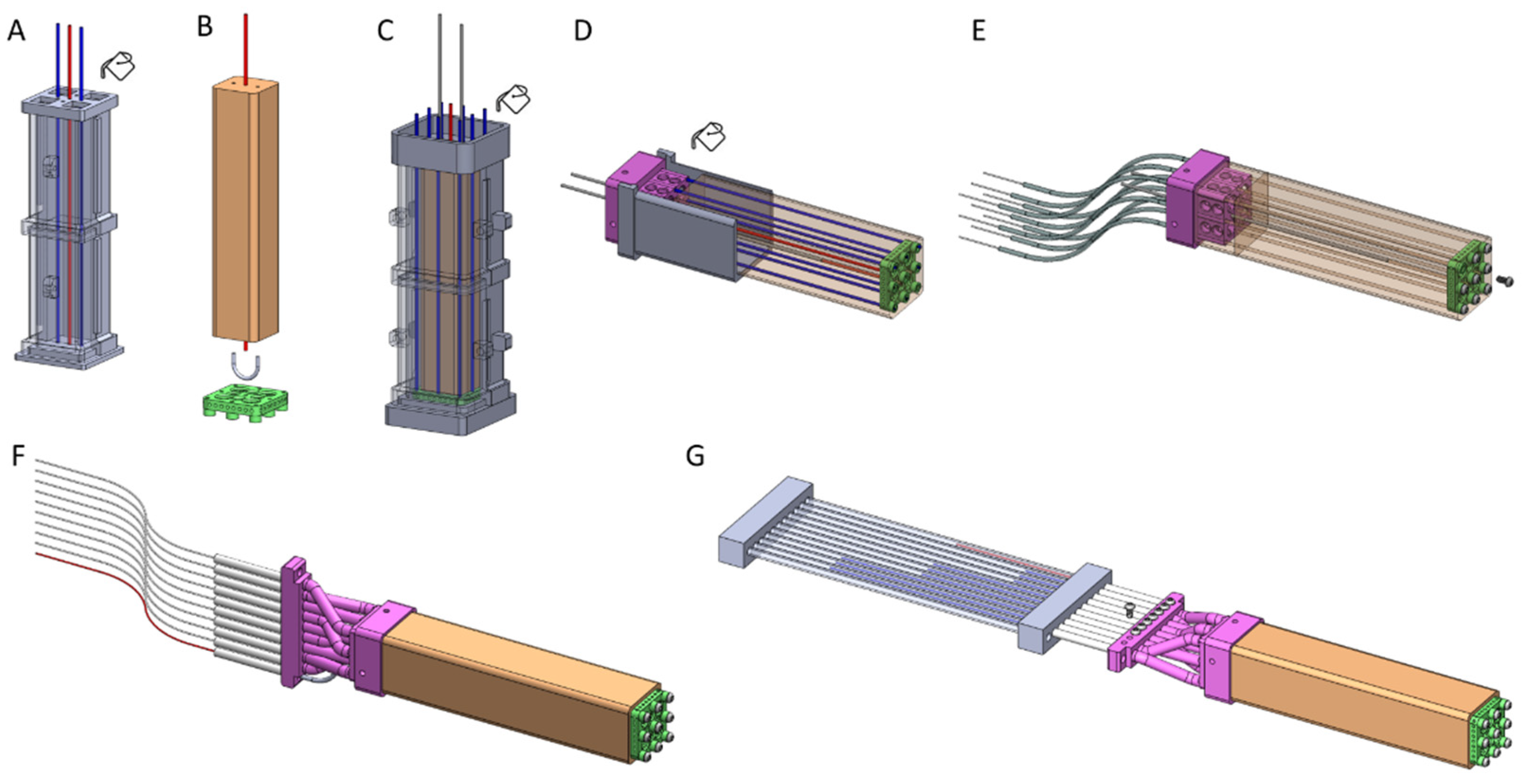
We present an elastomeric finger containing nine fiber-based displacement sensors, one integrated microfluidic pressure sensor, and the ability to be configured with one or more surface-mounted microfluidic pressure sensors. These are all monitored with a single digital camera. Simultaneous analysis of these sensors allows us to determine the state of the finger. In the fiber-based deformation sensor method (Figure 1A–C), we embedded a 3 × 3 matrix of fiber-based displacement sensors into the elastomeric finger. Each displacement sensor is composed of two main parts: fiber and tube. The fiber is a flexible but inextensible/incompressible nylon fiber. The tube is a flexible elastomeric void built into the bulk matrix of the finger. Fibers are fixed at the distal end of the finger and routed through tubes along the length of the finger and out to a display assembly (Figure 1B). A short length (marker) of each fiber inside the display assembly is painted black. This contrasts with the white background allowing a digital camera to record the relative motion of the marker. When the elastomeric finger is distorted (bent, twisted, stretched), each tube changes shape and is stretched or compressed based on the overall mechanics of the mode of distortion. The fiber (free to slide along the length of the tube) slides within the display assembly, where the marker position and motion are recorded by a digital camera. This is similar to the Bowden cable assembly, which transmits force in many bicycle handbrakes. In our device, however, the passive sensor is distorted based on external actuation and used to sense displacement, the reverse of Bowden cables. Multiple cable-based sensors are embedded along the dorsal, ventral, and medial surfaces of the soft robotic sensor (3 × 3 grid at the end of the finger in Figure 1A,B). Comparing relative motion between this grid of sensors allows differentiation between bending, stretching, and twist.
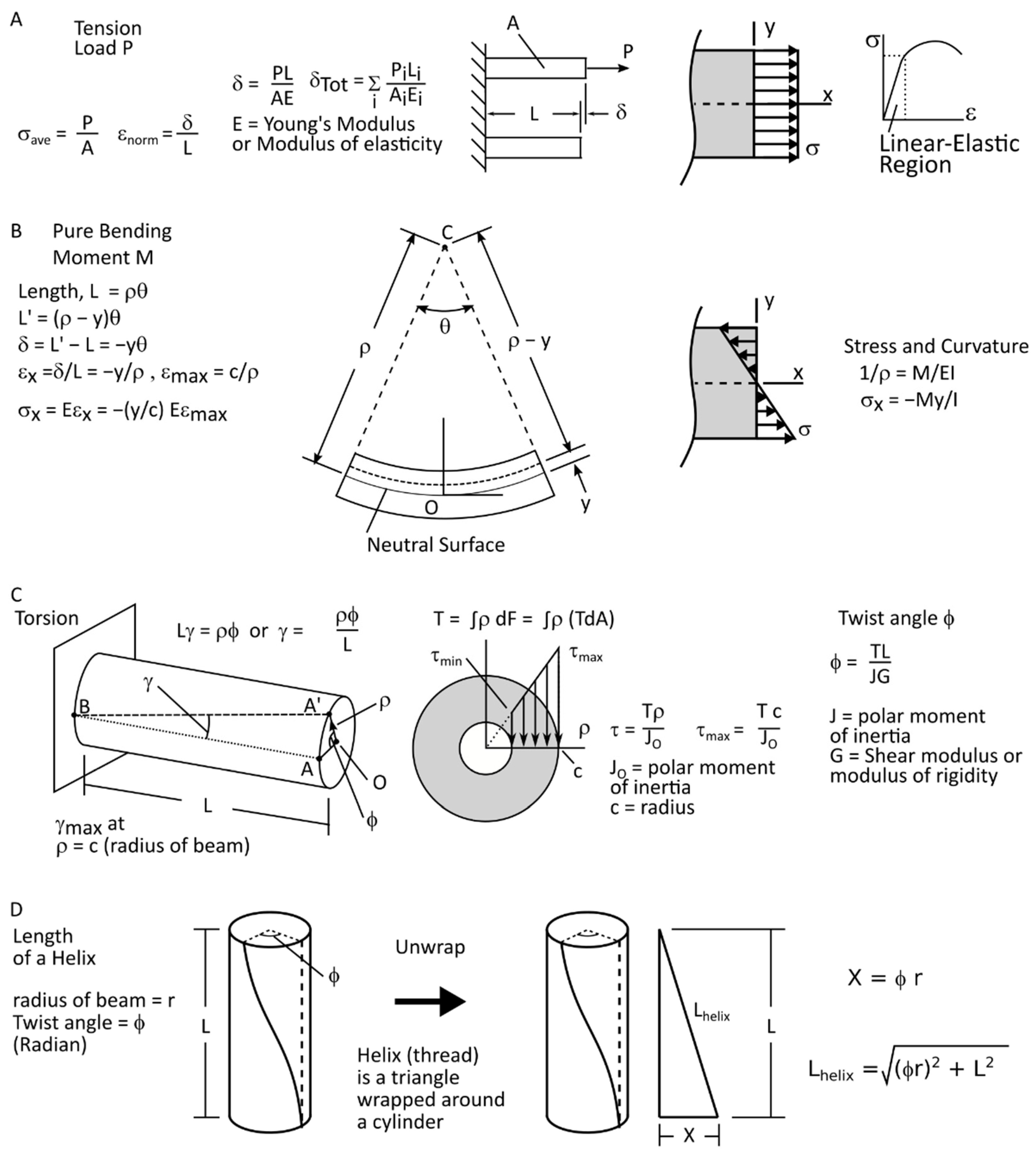
From Euler-Bernoulli beam theory and classical mechanics of materials, we know that beams experience stress and tension/compression throughout their cross-sections based on the mode of the applied loading (bending, tension/compression, twist, combined loading) [33]. Here we briefly summarize some primary beam deformation modes (Figure 2A) with more detail on derivation in Appendix A. For a detailed analysis of beam theory or mechanics of materials, many excellent texts are available [33,34,35,36].
First exploring simple elongation, we find that deformation is uniform across the cross-section, and proportional to the load applied (Figure 2A). Deformation follows the equation,
δ = P L A E
where δ is total displacement, P is applied load, L is total beam length, A is cross-section area, and E is Young’s Modulus.
In bending, material closer to the center of curvature (smaller bend radius) experiences compression, material farther from the center of curvature (larger bend radius) experiences tension, and material along the neutral axis experiences neither tension nor compression. Within the linear elastic range, stress from bending (Figure 2A) follows the equation,
σ x = M y I
where σ x is tensile or compressive stress, M is applied bending moment, y is the distance from the neutral surface (positive toward the center of curvature), and I is the second moment of inertia. The negative sign indicates compression toward the center of bending. Strain follows the equation,
ϵ x = y ρ
where ϵ x is the strain in the beam axis, y is the distance from the neutral surface (positive toward the center of curvature), and ρ is the radius of curvature of the bent beam. The negative indicates shortening toward the center of curvature.
Shearing stress due to torsion (Figure 2A) follows the equation,
τ = T ρ J
where τ is shear stress, T is applied torque, ρ is distance from the axis of rotation, and J is polar moment of inertia. The angle of twist follows the equation,
ϕ = T L J G
where ϕ is the total twist of the beam, L is beam length, J is the polar moment of inertia, and G is the shear modulus. We can find the change in length of a line (linear initially, helical after twist) parallel to the axis of the beam, a distance r from the twist axis. Initially of length L , the line becomes a helix after the beam twists by an angle ϕ , about its central axis. The helix (former line, now helix) length is found from the formula,
L h e l i x = L 2 + ( ϕ r ) 2
where L h e l i x is the length of the helix, ϕ is the angle of twist found above, L is the beam length, and r is the distance from twist axis (see Appendix A for derivation). Thus, we find the change in length of a fiber parallel to the longitudinal axis as,
Δ L = L h e l i x L
where Δ L is the change in length. With L and ϕ constant for any given beam and loading condition, we see that L h e l i x increases as r increases. Thus, the farther an element is from the axis of rotation, the more it will increase in length when experiencing a twist. Thus, fibers in the corners of a square cross-section will experience more displacement than fibers at the center of the square faces, and a fiber at the center of the square face will not elongate at all.
While these formulae hold for beams within the linear elastic region, the principles (while not necessarily the magnitudes) remain true in the large deformation regime. See Appendix A for details on the mechanics of materials described here, further figures on bending modes, and sign conventions [33].
While each fiber sensor gives us local deformation information, the true value of these devices comes when used in groups. Thus, they must be readily integrated at scale without undue hardware requirements. Traditional sensors require individual hardware for each sensor (Figure 2B top). These fiber sensors, however, require only the passive fiber components, and a single camera for all fibers (Figure 2B bottom). Then a single signal can be sent to the PC for video processing. Since video data consists of black markers moving horizontally across a white background, processing complexity is greatly reduced. For example, we select fiber sensors in the lower right and upper left corners of the finger (1 and 9 in front-view, Figure 2C). When the finger is bent upwards, 9 will indicate compression, but 1 will indicate tension. In elongation or twist, both will indicate tension. However, fibers 6 and 4 will indicate tension equal to 1 and 9 in extension, but less in twist. Expanding this example to the range of extension, bending, and twist scenarios, we configure a 3 × 3 matrix of fiber sensors, across the cross-section of the finger (as shown in Figure 2C). The combination of displacements allows us to interpret the deformation mode of the overall finger. For example, if the top three sensors are in compression, the middle three show no deformation, and the bottom three show tension, we can infer that the finger is being bent upwards. Only primary deformation modes are presented here. Mixed-mode deformations (combinations such as bend and twist) are left for future exploration. We present offline marker tracking and characterization of these sensors in the deformation modes discussed above, as well as real-time marker tracking, which we envision as a path toward real-time control of soft robot actuators.
In the integrated microfluidic pressure sensor method (
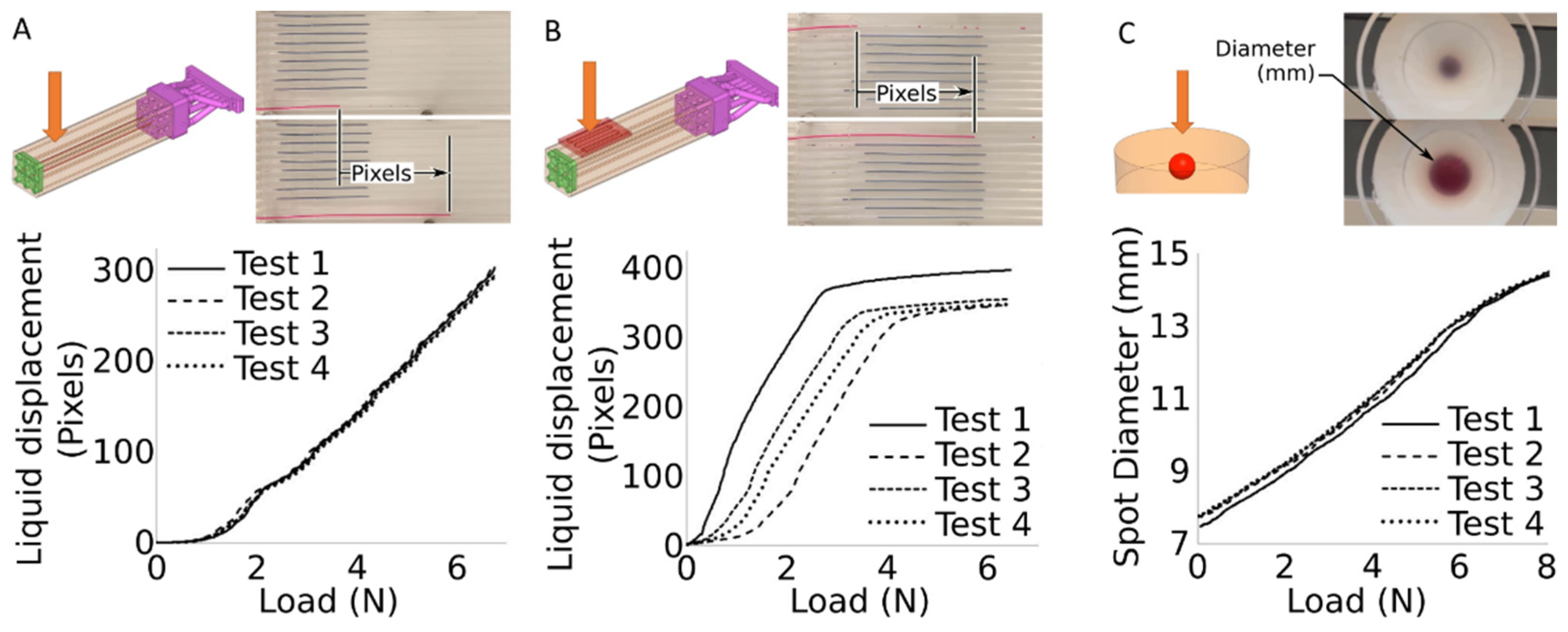
Figure 1D), we embed microfluidic channels into the elastomeric finger to sense the overall pressure exerted on the finger. This sensor consists of a sensing part and a transmission part, both filled with colored liquid. The sensing part is compressible and embedded along the length of the square column-shaped elastomeric finger. The transmission part consists of a flexible, incompressible tube routed through the display assembly. When force is applied to the sensing part, the chamber is compressed, reducing the volume of the sensor part. This forces the incompressible colored liquid out of the sensing part, through the transmission part, and across a display tube in the display assembly.
We also present a surface-mount pressure sensor (Figure 1E), which can be bonded (singularly or in batches) to the surface of the finger or any similar elastomeric device. This pressure sensor can be installed at any location on a multitude of elastomeric actuators and robotic systems. We present characterization data on one sensor to demonstrate its utility, not an exhaustive study of possible configuration or applications. Both microfluidic methods transmit to the same display assembly used to record fiber position, thus a single digital camera can capture data from fiber-based deformation sensors as well as microfluidic pressure sensors. The configuration we present records 11 sensors (nine fiber, one integrated microfluidic, and one surface mount microfluidic) captured by one digital camera, as that was sufficient for this proof of concept. An effort to minimize scale could greatly increase the number of discrete sensors possible with one camera.
Lastly, we present a color cell pressure sensor inspired by chromatophores in cephalopods [27]. Rather than mimicking this clever technique, we draw upon it for our inspiration [37] and flip the application from active modulation for camouflage to a passive sensor. Spherical cells of colored liquid are embedded in an elastomeric substrate. When the substrate undergoes external pressure, local deformation causes the spherical cells to deform, and become disk-like. Viewed from an axis normal to the disk plane, this causes the disks to appear larger than the original spheres. Thus, the applied force can be determined from the diameter of the disk.

2.1. Design and Fabrication

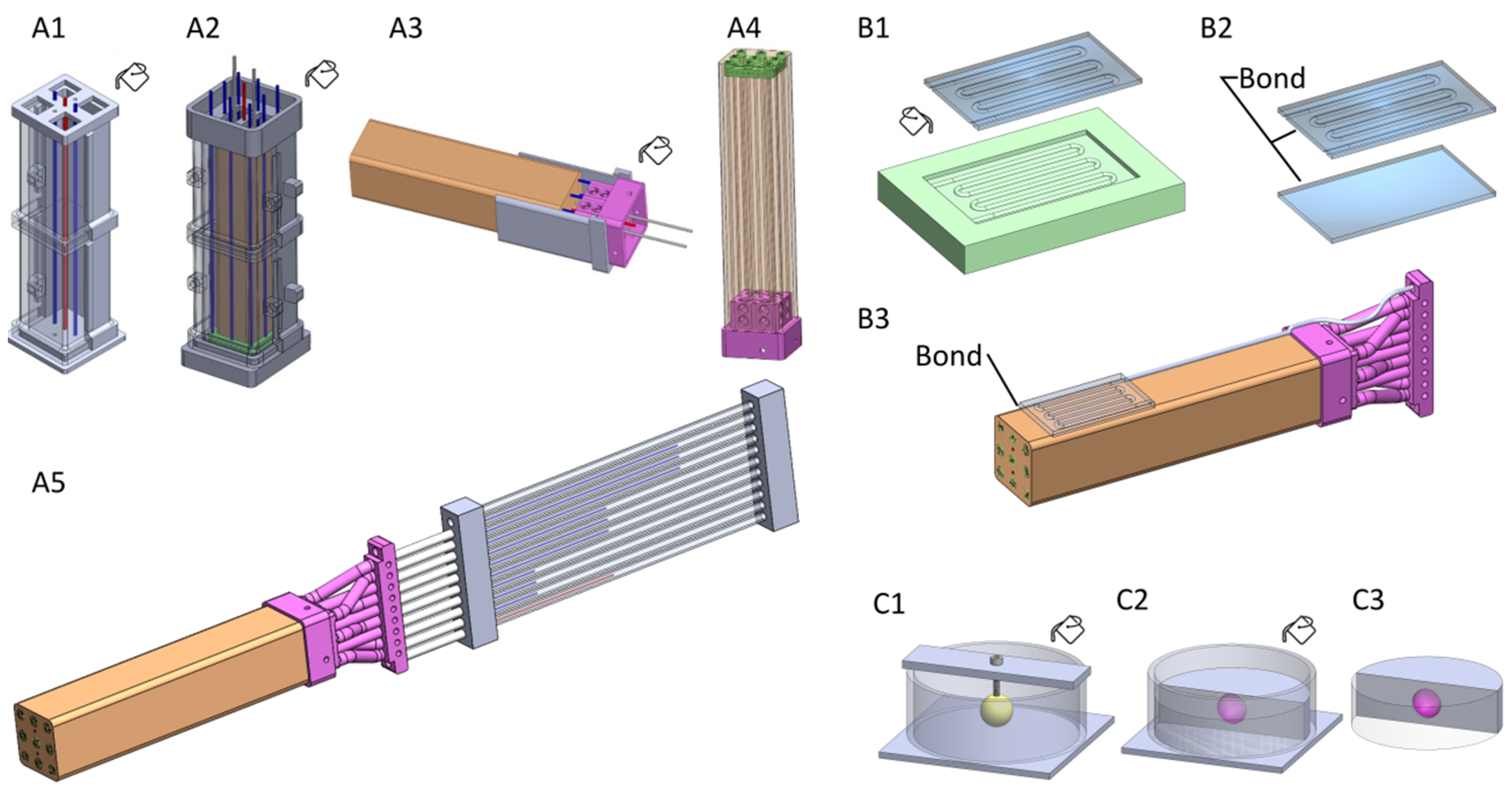
Fiber-based deformation sensor: (Since the elastomeric finger is fabricated as one device, the integrated microfluidic pressure sensor will be described in this section) Similar in concept to many soft robots, we fabricate our square column-shaped soft sensor (elastomeric finger) using multiple molding steps. The fabrication process is summarized in Figure 3A, with a detailed description in Appendix C. The assembly is fabricated using three molding steps and a final integration step. Mold 1. We used three plastic bars (diameter 0.9 mm) to create the center cable chamber and two microfluidic chambers. The matrix material of the finger is a readily available elastomer, Ecoflex 00-30 (Smooth-On, Inc. Macungie, PA, USA) in molds printed from a 3D Printer (Form 3, Formlabs, Somerville, MA, USA). Mold 2. Retaining the center plastic bar in the mold, we demolded the two other plastic bars. We used the silicon tube (inner diameter 0.5 mm, outer diameter 1 mm) to connect the microfluidic chambers on the top holes and extend the bottom holes. Then, we attached the top carrier to the center plastic bar and aligned it with the other eight plastic bars into the second mold. The top carrier embedded in the soft sensor provides a surface to fix the cables. Mold 3. We demolded the soft sensor from the second mold, keeping all the plastic bars and two silicon tubes inside the sensor, and then align them to the base holder. After alignment, we secured it into the final mold and connected the finger to the solid base holder once it cures. Integration. We inserted the high-strength fiber cables (Monofilament nylon thread, diameter 0.5 mm) into the soft sensor chambers, fixed them using screws on the top carrier, and injected the colored liquid into the microfluidic chambers.
Microfluidic pressure sensor: The design of the integrated microfluidic pressure sensor is described above, in the Fiber-based pressure sensor section, because it must be fabricated concurrently into one integrated unit. We present the integrated pressure sensor in the finger motif; it can, however, be designed into most actuator systems that use a matrix of molded elastomer. While this integrated sensor provides useful overall pressure of the soft finger, we developed a surface-mount microfluidic pressure sensor to expand sensing capabilities (Figure 3B). Similar in form to several existing surface-mount sensors, our technique uses the displacement of liquid rather than change in resistance in an ionogel [8,15] or liquid metal [18]. This surface-mount pressure sensor is similar in concept to a microfluidic embodiment of the Skinflow work by Hauser, Rossiter, et al. [38]. This surface mount sensor can be fabricated from elastomers of various durometers in different thicknesses to modulate sensitivity, and it can be mounted (singly or in groups) at various locations along the elastomeric finger or other actuators. Fluid displacement data can be interpreted in the same camera frame as the fiber-based actuator described above, thus expanding the sensing modes possible with this overall vision-based system.
Color cell pressure sensor: The final sensor technology presented here derives its inspiration from the chromatophores used by many cephalopods and some other animals to change their color and appearance. Chromatophore cells filled with pigment appear as small dark dots. To change perceived color, radial muscle fibers stretch the chromatophore cell from roughly spherical to a wide-thin disk shape of the same volume. Thus, when viewed from an axis normal to the disk-plane, the appearance changes from a small, dark dot in a near-transparent matrix to a larger colored disk. An array of these chromatophores in various colors allows the animal to present a variety of appearances. While cephalopods use their chromatophore cells to actively modulate their appearance, we invert this technique, using passive cells as sensors. Fabricated into an elastomeric matrix, external pressure causes these spherical cells to deform into disks in a plane normal to the applied force. When viewed from an axis normal to the disk plane, the diameter of the disk increases with applied force.

2.2. Vision Algorithms

An algorithm was designed to process two different possible image stream inputs: a real-time camera stream, or a previously recorded video. For the real-time processing, we used a video stream from a Raspberry Pi Camera Module 2, with the constraint of the camera being aligned such that the painted filaments are approximately parallel to the horizontal axis. The videos recorded on a separate device were filmed with the same constraint. To address alignment issues across multiple runs, boundaries are digitally positioned around each of the channels with the filaments in the camera frame (current frame for live stream, first frame for recorded videos) before beginning the algorithm.
The OpenCV Python library for image processing is used to facilitate detection in each frame. Each frame is first cropped to include only the boundaries and then converted to be in grayscale to accentuate differences in light and dark colors and to eliminate possible noise from reflection. Every pixel value within the frame is then scaled up to further accentuate the difference between the white background and the black filaments. The Canny edge detector algorithm is then used to determine the edges of the filaments, and the Hough Lines Probability algorithm returns the start and endpoint pixel coordinates of each line edge. The algorithm then iterates over each detected line and the endpoint furthest to the right within each boundary is recorded as a pixel location in a CSV. Further details are presented in Appendix B.

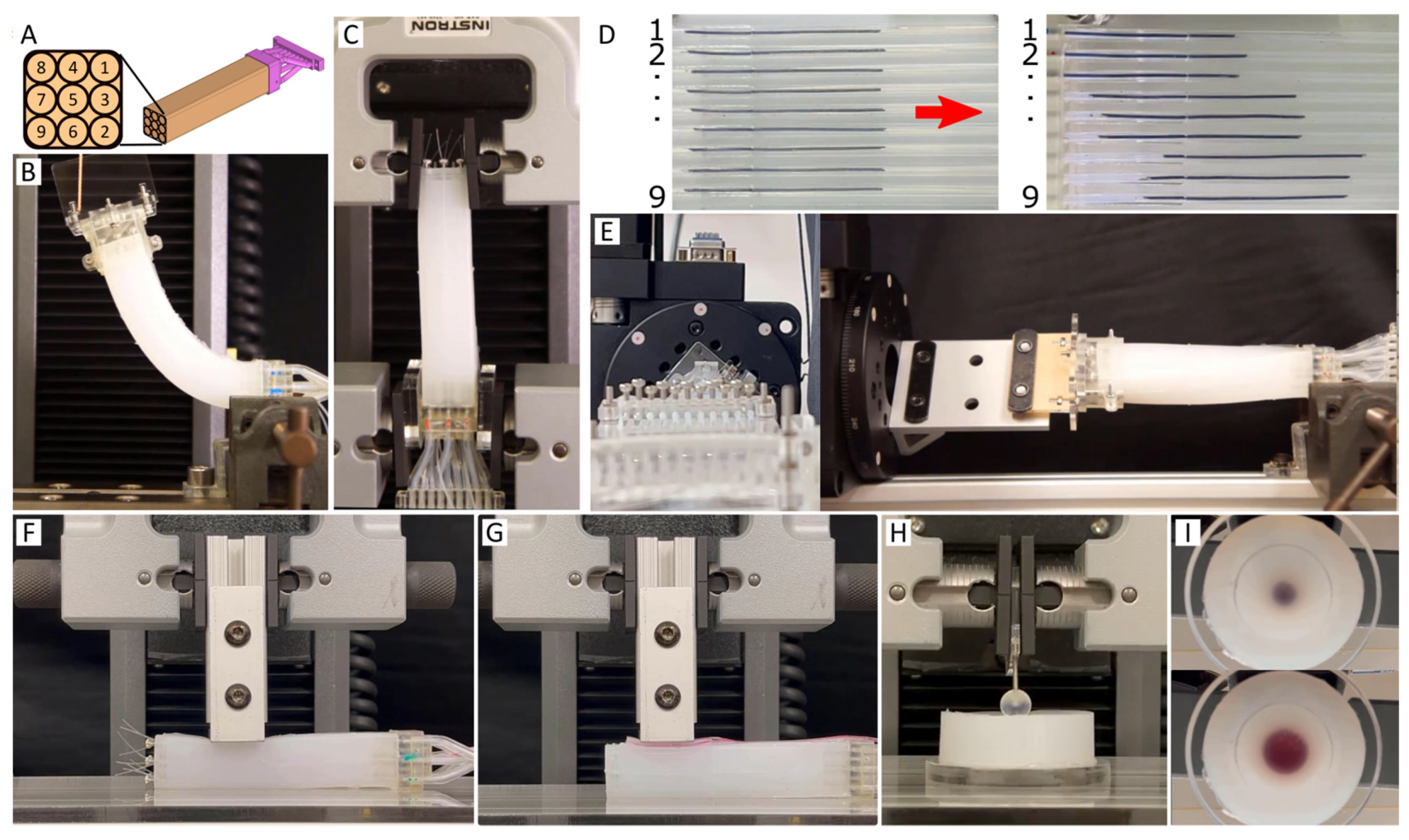
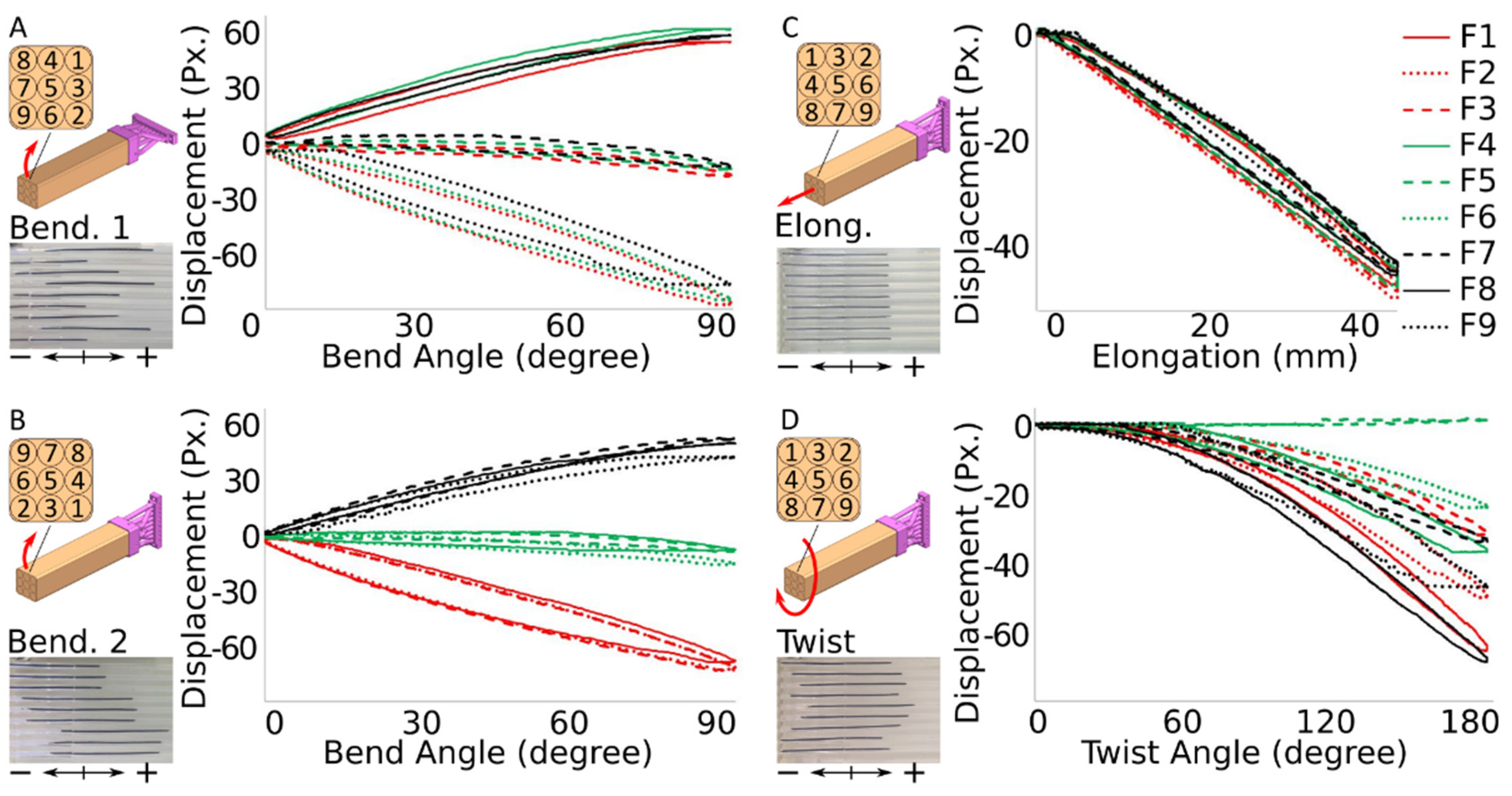
2.3. Sensor Characterization

We evaluated the elastomeric finger containing fiber-based displacement sensors and fluid-based pressure sensor in each actuation mode individually, with the understanding that mixed-mode sensing (elongation and twist combined, or bending along a non-primary axis) will be the goal of future development using the real-time vision algorithms described in Section 2.2. For the fiber-based sensor, separate characterization fixtures were employed for each mode of evaluation (bending, elongation, twist) as shown in Figure 4A, each mounted to an Instron 5943 tensile tester (Instron Co., Norwood, MA, USA). The same apparatus was used for bending 1 and bending 2, offset by 90° as illustrated in Figure 4A–E. Integrated microfluidic pressure sensor characterization (Figure 4F) and surface mount microfluidic pressure sensor characterization (Figure 4G) were performed on the same fixture, and chromatophore-inspired sensor characterization (Figure 4H,I) was performed on a separate fixture. Each test was performed four times to monitor repeatability.

3. Results

Data is divided into fiber-based deformation sensors, (estimating soft finger displacement) and fluid-based pressure sensors (microfluidic and color cells). Fiber-based sensor characterization investigates displacement of a 3 × 3 grid of fibers as described in the Methods section. Figure 5 presents fiber responses to displacement in two modes of bending (offset by 90°), extension, and twist (See also Supplementary Videos S1 and S2). Finger orientation and resulting fiber locations within the finger are shown in the illustration to the left of each graph. To achieve two modes of bending, the finger is rotated inside the mounting fixture 90° between Bending 1 and Bending 2, yielding a different fiber orientation. Fiber orientation for elongation and twist is also shown, but because these displacements are along the longitudinal axis, orientation does not affect results.

3.1. Fiber-Based Deformation Sensor

As the elastomeric finger undergoes displacement in the described mode, material distorts locally, consistent with theory from classical mechanics of materials (Appendix A). Fibers, attached at the distal end of the elastomeric finger are free to move inside their respective tubes (described in Section 1, Section 2), thus they do not elongate or compress. Rather they move along their tube and back through the display assembly. Thus, when the finger undergoes Bending direction 1 (Figure 5A), the top portion of the finger undergoes compression, the bottom undergoes tension, and the midplane sees little tension or compression. With the fiber configuration shown in Figure 5A, Bending 1 should cause the uppermost fibers to move farther into the display assembly (positive direction). The lower fibers should move out of the display assembly (negative direction) and fibers in the midplane should move very little at all. The graph in Figure 5A verifies this. Solid lines (fiber 1, 4, 8) are positive, dotted lines (fibers 2, 6, 9) are negative, and dashed lines (fiber 3, 5, 7) moved little at all. Due to the test setup (distal end of finger pulled upward and allowed to move laterally) some tension in the finger caused the midplane to stretch slightly, causing slight negative values in dashed lines.
When the finger was rotated 90° and Bending direction 2 was investigated (Figure 5B), similar results were seen for fibers based on the new orientation. In this configuration again, black lines (fibers 7, 8, 9) were those along the top edge of the finger, where the finger was in compression. These fibers moved into the display assembly (positive displacement). Similarly, red lines (fibers 1, 2, 3) were pulled out of the assembly, green lines (fibers 4, 5, 6) were little affected.
Tests in elongation (Figure 5C) were also as expected. As the elastomeric finger was elongated, all fibers move out of the display assembly, recorded as negative displacement. Experiments in twist (Figure 5D) also showed results consistent with classical mechanics of materials. Fibers at the corners, farthest radially from the central axis (fibers 1, 2, 8, 9) exhibited the most deformation, pulling the fibers out of the display assembly for negative displacement. Fibers along the flat of each surface (fibers 3, 4, 6, 7), closer to the neutral axis, exhibited less deformation, recorded as less-negative displacement. Finally, fiber 5 at the neutral axis exhibited almost no displacement at all.

3.2. Source of Hysteresis

One may initially be concerned with the hysteresis loop (actuation path does not overlay with release path, but instead creates a loop in bend angle, elongation, or twist vs. fiber displacement). If this were due to the internal properties of the fiber sensors, it would not negate the value of the sensing system, but it should be addressed. Analyzing still frames from our motion capture videos indicates that the actuation and release paths of the elastomeric finger do not trace out a similar path. In other words, the shape of the elastomeric finger is different at a given angle in the actuation (0° 90°) path than in the release (90° 0 ° ) path. Thus, it would be expected that the fibers sense different finger geometry based on the path. See Supplementary Video S4 for dynamic illustration overlaying actuation vs. release geometry.

3.3. Microfluidic Pressure Sensors

The elastomeric finger is configured with an integrated microfluidic pressure sensor along its entire length. Consisting of a liquid-filled microfluidic channel, this sensor is intended to sense the overall pressure state in the elastomeric finger. Thus, repeatability and range are highly desirable. Maximizing sensitivity (ability to perceive a light touch) is not required for this sensor. Figure 6A shows a very repeatable and linear response to forces up to eight Newton, with no sign of signal saturation (change in geometry precludes perception of increased applied load) over four trials. Figure 6B shows the sensor response of a surface-mounted pressure sensor over four trials. Such a sensor would be attached to the surface of the elastomeric finger to sense a desired (or undesired) contact at a particular location on the finger surface. Thus, for such a sensor, linearity and maximum force before saturation are not primary concerns. Rather, for this sensor, the ability to detect contact is of primary interest. While this sensor is shown to saturate with an applied force below four Newton, saturation is of little concern once contact is detected.
Finally, Figure 6C presents the behavior of the chromatophore-inspired fluidic pressure sensor. At applied loads, up to eight Newton, the radial expansion of the liquid cell is relatively repeatable and very linear. The technique has been demonstrated here using one liquid cell, but the technique could be expanded to any number of cells at varying depths, colors, and volumes to achieve a multitude of responses to pressure.

4. Discussion

We presented vision-based methods of sensing deformation and pressure in soft robots, each including only passive components inside the soft robot. First, we presented a fiber-based deformation sensor wherein local material displacement in a soft robot was transmitted to a remote display assembly and tracked by a digital camera. Next, we presented two fluidic sensors, wherein a pressure in a soft robot displaces liquid inside a microfluidic channel, which was transmitted back to the aforementioned display assembly. We presented an integrated microfluidic pressure sensor, by which the overall pressure state inside the body of a soft robot is tracked. Next, we presented a surface-mount pressure sensor to track contacts locally on the surface of a soft robot. Finally, we presented a color-cell pressure sensor. With this sensor, we flip the idea of a chromatophore (with which cephalopods actively stretch color cells from spheres into disks to modulate appearance for camouflage and other applications). In our application, the passive spherical color cell is embedded in an elastomeric matrix. When an external force is applied to the elastomer, the color cell is compressed in the direction normal to the force, expanding it radially. We characterized the radial expansion vs. applied force for one sample configuration.
We presented an elastomeric finger with nine embedded fiber deformation sensors, one integrated pressure sensor, and one surface-mounted pressure sensor. We characterized the fiber sensors in two orthogonal directions of bending, twist about the finger’s primary axis, and extension. All modes of deformation followed the responses expected from by mechanics of materials and beam theory. The integrated microfluidic pressure sensor demonstrated a highly repeatable response to externally applied pressure with no saturation detected at 7N externally applied force. The surface-mounted pressure sensor (to sense contact locally) sensed much smaller applied forces (0.05–0.3 N) but saturated when as little as 2N force was applied. As a contact sensor, early detection is more useful than high saturation levels. These encouraging results on a single elastomeric finger will provide a foundation upon which sensorized actuators will be developed based on actuator designs from our previous work [15,39].
While the very simple sensor designs presented here have value individually, the key contribution of this work is that the sensors are fundamentally designed to be used in groups. Intended to be designed into a soft robot at the system level, a properly configured array of these deformation and pressure sensors can give state awareness far beyond that of individual sensors. Most sensors used in soft robots (and many sensors in general) vary in resistance or capacitance in response to a change in a physical parameter such as length, bend angle, or contact pressure. Each sensor requires wiring, electronic circuitry, and a dedicated input to a data acquisition system before the resulting signal is sent to a computer. Five sensors require five times the infrastructure. With our presented method, a digital camera records the movement of markers on fiber sensors and colored liquid in microfluidic channels. Thus, dozens of markers and fluid channels can be monitored almost as easily as one. Other camera-based soft robot state-estimation systems exist, but they primarily record the pose of the robot directly, thus requiring specific lighting conditions, unobstructed line-of-sight access to all parts of the robot.
The elastomeric finger we presented used nine fiber sensors to determine its pose, and two fluidic sensors to determine overall and local pressure states. By configuring fibers in a 3 × 3 matrix, we used the theories put forth in classical Mechanics of Materials (See Appendix A) to determine pose during states of bending in both primary planes, twist about the primary axis, and elongation along the primary axis. While the presented work was on a finger designed specifically to illustrate adherence to classical mechanics of materials theory, this state estimation could be applied to a range of soft actuators and soft robots in general. As stated above, we plan to use this technique in an actuator design similar to our previous soft finger [15,39] with a roughly square cross-section. These fiber and fluidic sensors could be used in many soft robots with actuators having rectangular, round, or trapezoidal cross-sections, requiring sensors to be placed at based on beam theory for that cross-section. With their innate under-actuation and deformability, defining the pose of a soft robot with reasonable accuracy requires far more sensors than do traditional robots. One can readily imagine a soft robot requiring nine sensors (3 × 3 matrix) for EACH actuator to estimate its pose. Thus, a three-fingered gripper would require 27 sensors, a simple quadruped would require 36, and a more complex robot would require many more. The circuitry and wiring required for this many discrete electrical sensors would quickly become burdensome. With our method, passive sensors are all routed back to one central display assembly and recorded by one digital camera. While we present 11 sensors in the display assembly, this number was chosen as it was the number required to characterize the soft finger (nine deformation and two pressure sensors). With our method, any upgrading (to increase sampling frequency or resolution) would be contained to the camera system, while upgrading dozens of electrical sensors would also be a sizeable task. With our method, many fibers could be routed back to one remote display assembly, where a single digital camera could track the motion of all markers in a controlled environment, optimally lit for contrast and marker tracking.

Supplementary Materials

The following are available online at https://www.mdpi.com/article/10.3390/electronics10243166/s1, Video S1: Fiber-based Sensor for Single-mode Deformations, Video S2: Fluid-based Pressure Sensors Deformation, Video S3: Vision Algorithms and Image Processing, Video S4: Fiber-based Sensor Overlaying Actuation vs. Release Geometry, Video S5: Multi-mode Free Movement Deformation Demo.

Author Contributions

Conceptualization and investigation, K.-Y.L., A.G.-G. and M.W.; methodology, K.-Y.L., A.G.-G. and M.W.; project administration and supervision, M.W.; validation, K.-Y.L., A.G.-G.; programming, machine vision, A.G.-G.; writing, review, and editing, K.-Y.L., A.G.-G. and M.W. All authors have read and agreed to the published version of the manuscript.

Funding

This research was funded by the Hellman Fellow Program 2020.

Conflicts of Interest

The authors declare no conflict of interest.

Appendix A

Euler-Bernoulli beam theory and Mechanics of materials, brief overview,
Figure A1. Mechanics of materials. (A). Beam in tension. (B). Beam in bending. (C). Beam in torsion. (D). length of a helix.
Electronics 10 03166 g0a1
Considering first, a beam in tension (Figure A1A), on a beam of length L with uniform cross section, the beam will lengthen proportionately with the load applied. The equation governing this extension is:
δ = P L A E
where δ is total displacement, P is applied load, L is total beam length, A is cross section area, and E is Young’s Modulus. Notice, in this loading scenario, the extension depends only on cross section AREA, not the shape of the member. Note, also, Young’s modulus is a mechanical property of the material. When we look at the stress-strain curve for many materials, they exhibit a region of linearity (strain is proportional to applied stress, so relationship is a straight line through the origin) and a nonlinear region. A sample stress strain curve representative of many engineering materials (qualitative, no numbers included) is shown in Figure A1A. The formulae presented here hold in the linear portion of the stress strain curve, governed by the young’s modulus. Outside this region, direct quantitative relationships can no longer be applied with certainty, thus we use these as general rules to demonstrate the phenomena, not develop quantitative relationships.
When exposed to a bending moment, a beam forms a circular arc as shown in Figure A1B. As shown, the center of this circular arc lies above the arc. The portions of the arc closest to the center of curvature experience compression. The portion farthest from the center of curvature experience tension. Somewhere between the region of maximum compression and the region of maximum tension lies a region of neither tension nor compression. We call this the neutral surface. Stress along the cross section of a beam in bending follows the relationship
Within the linear elastic range, stress from bending (Figure A2B) follows the equation,
σ x = M y I
where σ x is tensile or compressive stress, M is applied bending moment, y is distance from neutral surface (positive toward the center of curvature), and I is second moment of inertia. The negative sign indicates compression toward the center of bending. Strain follows the equation,
ϵ x = y ρ
where ϵ x is strain in the beam axis, y is distance from the neutral surface (positive toward the center of curvature), and ρ is radius of curvature of the bent beam. The negative indicates compression toward the center of curvature.
Shearing stress due to torsion (Figure A1C) follows the equation,
τ = T ρ J
where τ is shear stress, T is applied torque, ρ is distance from the axis of rotation, and J is polar moment of inertia. Angle of twist follows the equation,
ϕ = T L J G
where ϕ is total twist of the beam,   L is beam length, J is polar moment of inertia, and G is shear modulus. We can find the change in length of a line (linear initially, helical after twist) parallel to the axis of the beam, a distance r from the twist axis. First, consider the shape of a helix (similar to a screw thread). A helix can be thought of as a right triangle or ramp wrapped around a cylinder. The height of this triangle is the length of the cylinder. The width of the triangle is the length of the portion wrapped about the cylinder. Angle of Twist is ϕ as we calculated in (A5). Therefore, width of the triangle X is ( ϕ / 2 π ) × ( 2 π r ) = r ϕ . Thus, the length of the helix is the length of the hypotenuse of a right triangle of sides L and r ϕ . Initially of length L , after twisting an angle ϕ , the helix (former line, now helix) has a length found from the formula,
L h e l i x = L 2 + ( r ϕ ) 2
where L h e l i x is the length of the helix, ϕ is angle of twist found above, L is beam length, and r is distance from twist axis (see Appendix A for derivation). Thus, we find the change in length of a fiber parallel to the longitudinal axis as
Δ L = L h e l i x L
where Δ L is the change in length. With L and ϕ constant for any given beam and loading condition, we see that L h e l i x increases as r increases. Thus, the farther an element is from the axis of rotation, the more it will increase in length when experiencing twist. Thus fibers in the corners of a square cross section will experience more displacement than fibers at the center of the square faces, and a fiber at the center of the square face will not elongate at all.

Appendix B

A Python script was created to automatically process the videos to extract position data. The first frame of the recorded video is accessed and then saved using the deepcopy function to preserve the original state. The frame then goes through a loop where the user moves lines, displayed with the OpenCv line function, vertically and horizontally to create the boundary for each cable’s channel, as well as flip the frame along the y axis if the orientation is not correct. Once the user has completed preprocessing the frame, the selected boundaries and orientation are recorded. The saved copy of the first frame is then accessed, and the object tracking algorithm begins. Each pixel of each frame is initially encoded as three individual bytes representing the intensity of red, green, and blue hues. A new frame with cropped dimensions around the selected boundaries is then constructed where the value of each pixel is a single byte value calculated with the following formula:
p i x e l g r a y = 1.6   ( p i x e l r e d + p i x e l g r e e n + p i x e l b l u e ) 3
The new frame then goes through the Canny algorithm. The Canny algorithm takes the numerical derivative of pixels in the horizontal and vertical directions and creates a gradient two-dimensional array [40]. To reduce noise, each index is compared against its neighbors to check if it is a local maximum. The maximums are set to 1, and all other indices are suppressed to 0. The binary two-dimensional array then goes through the Probabilistic Hough Lines Transform algorithm. The Probabilistic Hough Lines Transform algorithm processes the binary array by converting the position of a sufficiently sized random subset of the indices ( x i ,   y i ) with the value 1 from Cartesian coordinates to Hough Space lines with the following equation [41]:
ρ = x i cos θ + y i sin θ
The algorithm them iterates over θ in the range [ 0 ,   180 ] degrees, and for every intersection between two or more lines ( θ 0 , ρ 0 ) , the total number of intersections is recorded. If the number of intersections is larger than a set threshold, then the Hough Space coordinates are converted to Cartesian coordinate line endpoints with the equations [41]
x 1 , 2 = ( cos ( θ 0 ) ρ 0 ) 1000 sin ( θ 0 ) y 1 , 2 = ( sin ( θ 0 ) ρ 0 ) ± 1000 cos ( θ 0 )
These equations yield lines that span the entire frame. The algorithm then isolates the subsection of these lines that correspond to continuous high values from the binary array. The script then loops through each user-defined boundary and extracts the subset of fully contained lines. The rightmost end point of each line is recorded in the comma separated value (csv) file and the next frame is then loaded.

Appendix C

The fabrication of an elastomeric finger assembly consists of three molding steps, several cable routing steps, fastening steps, and final integration/assembly as shown in Figure A2. First, a mold (Mold 1) is assembled; including three 0.8mm diameter, semi-rigid cylinder parts (Bars). These bars will contain the central fiber (Fiber 5) and liquid for the microfluidic pressure sensor. Mold 1 is filled with elastomer (Ecoflex 30) and cured at 60 °C for at least 40 min (Figure A2A). The elastomeric construct is removed from Mold 1, the two bars for the microfluidic pressure sensor are removed, a short piece of silicone tubing is inserted, connecting the two microfluidic channels, and an end-cap (shown in green) is secured to the distal end of the elastomer (Figure A2B). The construct is installed into another mold (Mold 2) and instrumented with eight more bars which will contain the other eight fibers (1–4, 6–9). Microfluidic channels are instrumented with temporary PTFE tubing to prevent elastomer ingress. Mold 2 is filled with Ecoflex 30 and cured at 60 °C for at least 40 min (Figure A2C). The construct is removed from Mold 2, and temporary PTFE tubing is removed. At the proximal end of the device, the two microfluidic channels are instrumented with silicone tubing (shown in gray) which are routed through the base cap (shown in pink) and exit the system. The construct is assembled into a mold (Mold 3), filled with Ecoflex 30, and cured at 60 °C for at least 40 min (Figure A2D). Mold 3 is removed, nylon fibers are routed through each of the nine fiber holes, and the fibers are fastened with screws to the distal end of the finger (Figure A2E). Fibers and tubing for the microfluidic channel are routed through a base holder (shown in pink), and the base holder is mounted to the finger assembly. Tubing for the microfluidic channel is routed to the hole available just below Fiber 9 (shown in red). An additional hole is available above Fiber 1 for a surface-mount microfluidic pressure sensor if one is present (Figure A2F). The display assembly is laid out with components of laser-cut acrylic. A small region of each fiber (~2 cm) is painted black near the entry of the display assembly. All fibers and the microfluidic pressure sensor are routed through the display assembly. Display assembly and base holder are fastened to fiber tubes with button head screws (Figure A2G).
Figure A2. Elastomeric finger fabrication process. (A). Mold 1. (B). Connect vasculature to microfluidic pressure sensor. (C). Mold 2. (D). Mold 3. (E). Connect fibers. (F). Routing cables through base holder. (G). Integrate finger with Display Assembly.
Electronics 10 03166 g0a2

References

  1. Lynch, K.M.; Park, F.C. Modern Robotics: Mechanics, Planning, and Control; Cambridge University Press: New York, NY, USA, 2018. [Google Scholar]
  2. Murray, R.M.; Li, Z.; Sastry, S.S.; Sastry, S.S. A Mathematical Introduction to Robotic Manipulation; CRC: Boca Raton, FL, USA, 1994. [Google Scholar]
  3. Homberg, B.S.; Katzschmann, R.K.; Dogar, M.R.; Rus, D. Robust Proprioceptive Grasping with a Soft Robot Hand. Auton. Robot. 2019, 43, 681–696. [Google Scholar] [CrossRef] [Green Version]
  4. Wu, Q.; Yang, X.; Wu, Y.; Zhou, Z.; Wang, J.; Zhang, B.; Luo, Y.; Chepinskiy, S.A.; Zhilenkov, A.A. A Novel Underwater Bipedal Walking Soft Robot Bio-Inspired by the Coconut Octopus. Bioinspir. Biomim. 2021, 16, 046007. [Google Scholar] [CrossRef] [PubMed]
  5. Li, D.; Dornadula, V.; Lin, K.; Wehner, M. Position Control for Soft Actuators, Next Steps toward Inherently Safe Interaction. Electronics 2021, 10, 1116. [Google Scholar] [CrossRef]
  6. Muth, J.T.; Vogt, D.M.; Truby, R.L.; Mengüç, Y.; Kolesky, D.B.; Wood, R.J.; Lewis, J.A. Embedded 3D Printing of Strain Sensors within Highly Stretchable Elastomers. Adv. Mater. 2014, 26, 6307–6312. [Google Scholar] [CrossRef]
  7. Roberts, P.; Damian, D.D.; Shan, W.; Lu, T.; Majidi, C. Soft-Matter Capacitive Sensor for Measuring Shear and Pressure Deformation. In Proceedings of the 2013 IEEE International Conference on Robotics and Automation, Karlsruhe, Germany, 6–10 May 2013; pp. 3529–3534. [Google Scholar]
  8. Boivin, M.; Milutinović, D.; Wehner, M. Movement Error Based Control for a Firm Touch of a Soft Somatosensitive Actuator. In Proceedings of the 2019 American Control Conference (ACC), Philadelphia, PA, USA, 10–12 July 2019; pp. 7–12. [Google Scholar]
  9. Zhao, H.; O’Brien, K.; Li, S.; Shepherd, R. Optoelectronically Innervated Soft Prosthetic Hand via Stretchable Optical Waveguides. Sci. Robot. 2016, 1, eaai7529. [Google Scholar] [CrossRef] [PubMed] [Green Version]
  10. Cho, G.-S.; Park, Y.-J. Soft Gripper with EGaIn Soft Sensor for Detecting Grasp Status. Appl. Sci. 2021, 11, 6957. [Google Scholar] [CrossRef]
  11. Kim, T.; Lee, S.; Hong, T.; Shin, G.; Kim, T.; Park, Y.-L. Heterogeneous Sensing in a Multifunctional Soft Sensor for Human-Robot Interfaces. Sci. Robot. 2020, 5, eabc6878. [Google Scholar] [CrossRef]
  12. Hammond, F.L.; Mengüç, Y.; Wood, R.J. Toward a Modular Soft Sensor-Embedded Glove for Human Hand Motion and Tactile Pressure Measurement. In Proceedings of the 2014 IEEE/RSJ International Conference on Intelligent Robots and Systems, Chicago, IL, USA, 14–18 September 2014; pp. 4000–4007. [Google Scholar]
  13. Chossat, J.-B.; Park, Y.-L.; Wood, R.J.; Duchaine, V. A Soft Strain Sensor Based on Ionic and Metal Liquids. IEEE Sens. J. 2013, 13, 3405–3414. [Google Scholar] [CrossRef]
  14. Daalkhaijav, U.; Yirmibesoglu, O.D.; Walker, S.; Mengüç, Y. Rheological Modification of Liquid Metal for Additive Manufacturing of Stretchable Electronics. Adv. Mater. Technol. 2018, 3, 1700351. [Google Scholar] [CrossRef]
  15. Truby, R.L.; Wehner, M.; Grosskopf, A.K.; Vogt, D.M.; Uzel, S.G.; Wood, R.J.; Lewis, J.A. Soft Somatosensitive Actuators via Embedded 3D Printing. Adv. Mater. 2018, 30, 1706383. [Google Scholar] [CrossRef] [PubMed] [Green Version]
  16. Vogt, D.; Menguc, Y.; Park, Y.-L.; Wehner, M.; Kramer, R.K.; Majidi, C.; Jentoft, L.P.; Tenzer, Y.; Howe, R.D.; Wood, R.J. Progress in Soft, Flexible, and Stretchable Sensing Systems. In Proceedings of the Proceedings of the International Workshop on Research Frontiers in Electronics Skin Technology at ICRA, Karlsruhe, Germany, 6–10 May 2013; Volume 13. [Google Scholar]
  17. Truby, R.L. Designing Soft Robots as Robotic Materials. Acc. Mater. Res. 2021, 2, 854–857. [Google Scholar] [CrossRef]
  18. Park, Y.-L.; Chen, B.-R.; Wood, R.J. Design and Fabrication of Soft Artificial Skin Using Embedded Microchannels and Liquid Conductors. IEEE Sens. J. 2012, 12, 2711–2718. [Google Scholar] [CrossRef]
  19. Gerboni, G.; Diodato, A.; Ciuti, G.; Cianchetti, M.; Menciassi, A. Feedback Control of Soft Robot Actuators via Commercial Flex Bend Sensors. IEEE/ASME Trans. Mechatron. 2017, 22, 1881–1888. [Google Scholar] [CrossRef]
  20. Fast Probabilistic 3-D Curvature Proprioception with a Magnetic Soft Sensor. Available online: https://ieeexplore.ieee.org/abstract/document/9551572?casa_token=PeqhRYVUnWwAAAAA:pzzoRF3McivXXhlOd56BhlouOZBsG9mZd8TqIldmzRxRRAZuQLN9CIVlOfbpp7r-4oekd3U2Yw (accessed on 27 October 2021).
  21. McInroe, B.W.; Chen, C.L.; Goldberg, K.Y.; Goldberg, K.Y.; Bajcsy, R.; Fearing, R.S. Towards a Soft Fingertip with Integrated Sensing and Actuation. In Proceedings of the 2018 IEEE/RSJ International Conference on Intelligent Robots and Systems (IROS), Madrid, Spain, 1–5 October 2018; pp. 6437–6444. [Google Scholar]
  22. Tapia, J.; Knoop, E.; Mutný, M.; Otaduy, M.A.; Bächer, M. MakeSense: Automated Sensor Design for Proprioceptive Soft Robots. Soft Robot. 2020, 7, 332–345. [Google Scholar] [CrossRef]
  23. Otero, T.F. Towards Artificial Proprioception from Artificial Muscles Constituted by Self-Sensing Multi-Step Electrochemical Macromolecular Motors. Electrochim. Acta 2021, 368, 137576. [Google Scholar] [CrossRef]
  24. Shih, B.; Shah, D.; Li, J.; Thuruthel, T.G.; Park, Y.-L.; Iida, F.; Bao, Z.; Kramer-Bottiglio, R.; Tolley, M.T. Electronic Skins and Machine Learning for Intelligent Soft Robots. Sci. Robot. 2020, 5, eaaz9239. [Google Scholar] [CrossRef] [PubMed]
  25. Holmes, P.; Full, R.J.; Koditschek, D.; Guckenheimer, J. The Dynamics of Legged Locomotion: Models, Analyses, and Challenges. SIAM Rev. 2006, 48, 207–304. [Google Scholar] [CrossRef] [Green Version]
  26. Dahiya, R.S.; Mittendorfer, P.; Valle, M.; Cheng, G.; Lumelsky, V.J. Directions Toward Effective Utilization of Tactile Skin: A Review. IEEE Sens. J. 2013, 13, 4121–4138. [Google Scholar] [CrossRef]
  27. Florey, E. Ultrastructure and Function of Cephalopod Chromatophores. Am. Zool. 1969, 9, 429–442. [Google Scholar] [CrossRef] [Green Version]
  28. Cloney, R.A.; Brocco, S.L. Chromatophore Organs, Reflector Cells, Iridocytes and Leucophores in Cephalopods. Am. Zool. 1983, 23, 581–592. [Google Scholar] [CrossRef]
  29. Williams, T.L.; Senft, S.L.; Yeo, J.; Martín-Martínez, F.J.; Kuzirian, A.M.; Martin, C.A.; DiBona, C.W.; Chen, C.-T.; Dinneen, S.R.; Nguyen, H.T.; et al. Dynamic Pigmentary and Structural Coloration within Cephalopod Chromatophore Organs. Nat. Commun. 2019, 10, 1004. [Google Scholar] [CrossRef] [PubMed]
  30. Giordano, G.; Carlotti, M.; Mazzolai, B. A Perspective on Cephalopods Mimicry and Bioinspired Technologies toward Proprioceptive Autonomous Soft Robots. Adv. Mater. Technol. 2021, 6, 2100437. [Google Scholar] [CrossRef]
  31. Zeng, S.; Zhang, D.; Huang, W.; Wang, Z.; Freire, S.G.; Yu, X.; Smith, A.T.; Huang, E.Y.; Nguon, H.; Sun, L. Bio-Inspired Sensitive and Reversible Mechanochromisms via Strain-Dependent Cracks and Folds. Nat. Commun. 2016, 7, 11802. [Google Scholar] [CrossRef] [PubMed]
  32. Rossiter, J.; Yap, B.; Conn, A. Biomimetic Chromatophores for Camouflage and Soft Active Surfaces. Bioinspir. Biomim. 2012, 7, 036009. [Google Scholar] [CrossRef]
  33. Beer, F.P.; Johnston, E.R.; DeWolf, J.T.; Mazurek, D.F. Mechanics of Materials; McGraw-Hill Companies: New York, NY, USA, 1992. [Google Scholar]
  34. Timoshenko, S. History of Strength of Materials: With a Brief Account of the History of Theory of Elasticity and Theory of Structures; Courier Corporation: North Chelmsford, MA, USA, 1983. [Google Scholar]
  35. Young, W.C.; Budynas, R.G.; Sadegh, A.M. Roark’s Formulas for Stress and Strain; McGraw-Hill Education: New York, NY, USA, 2012. [Google Scholar]
  36. Boresi, A.P.; Schmidt, R.J.; Sidebottom, O.M. Advanced Mechanics of Materials; Wiley: New York, NY, USA, 1985; Volume 6. [Google Scholar]
  37. Aziz, M.S.; El sherif, A.Y. Biomimicry as an Approach for Bio-Inspired Structure with the Aid of Computation. Alex. Eng. J. 2016, 55, 707–714. [Google Scholar] [CrossRef] [Green Version]
  38. Soter, G.; Garrad, M.; Conn, A.T.; Hauser, H.; Rossiter, J. Skinflow: A Soft Robotic Skin Based on Fluidic Transmission. In Proceedings of the 2019 2nd IEEE International Conference on Soft Robotics (RoboSoft), Seoul, Korea, 14–18 April 2019; pp. 355–360. [Google Scholar]
  39. Lin, K.-Y.; Gupta, S.K. Soft Fingers with Controllable Compliance to Enable Realization of Low Cost Grippers. In Proceedings of the Biomimetic and Biohybrid Systems: 6th International Conference, Living Machines, Stanford, CA, USA, 26–28 July 2017; Mangan, M., Cutkosky, M., Mura, A., Verschure, P.F.M.J., Prescott, T., Lepora, N., Eds.; Springer International Publishing: Cham, Switzerland, 2017; pp. 544–550. [Google Scholar]
  40. OpenCV. Canny Edge Detection. Available online: https://docs.opencv.org/3.4/da/d22/tutorial_py_canny.html (accessed on 16 November 2021).
  41. Lee, S. Lines Detection with Hough Transform. Available online: https://towardsdatascience.com/lines-detection-with-hough-transform-84020b3b1549 (accessed on 16 November 2021).
Figure 1. Soft sensors. (A). Elastomeric finger containing a microfluidic pressure sensor and nine fiber-based deformation sensors to sense pressure, bending, elongation, and twist. (B). Illustration of the elastomeric finger with fiber and fluidic sensors routed through the finger to a display assembly, where sensor positions are read by a digital camera. (C). Fiber-based deformation sensors, relaxed and bent states. Finger (top) and fiber states (bottom). (Stills from Video S1.) (D). Integrated microfluidic pressure sensor, senses overall pressure. (E). Surface-mount pressure sensor senses contact locally on the finger’s surface. (F). Cephalopod-Chromatophore inspired color cell pressure sensor. External force causes the cell to change shape from spherical to a disk shape, changing disk diameter.
Electronics 10 03166 g001
Figure 2. Fiber sensors, underlying concepts. (A). Mechanics of materials in elongation, bending, and twist. (B). Traditional vs. soft sensors. Traditional (top), each sensor requires separate electronics and support. Bottom, multiple fiber sensors all routed back to display assembly. One camera records all sensors. One actuator is indicated in blue. Two additional actuators are indicated in red. (C). CAD of assembly with the first (blue) actuator and two additional (red) actuators. Note, Camera records display assembly, not soft actuators for reduced complexity motion capture of many sensors at once.
Electronics 10 03166 g002
Figure 3. Fabrication. (A). Elastomeric finger containing fiber-based displacement sensor and integrated fluid pressure sensors. (A1A3). An elastomeric finger is fabricated in three mold steps, containing channels for the nine fiber sensors and an integrated fluid pressure sensor. Molds are shown in gray. (A4). Finished elastomeric finger, transparent representation to illustrate internal vasculature. (A5). A finger is instrumented with fibers and integrated with the display assembly. (B). Surface mount liquid pressure sensor is molded (B1), bonded to a base layer (B2), then bonded to an elastomeric finger, and infilled with colored water (B3). (C). Chromatophore cell is molded into an elastomeric substrate and infilled with colored water (C1), then sealed with elastomer (C2) yielding a final sensor (C3).
Electronics 10 03166 g003
Figure 4. Test fixtures. (AE) fiber-based displacement sensors, (FI) fluid-based pressure sensors (A). Fiber sensor configuration. (B). Bend test setup. Elastomeric finger mounted horizontally, pulled from neutral to deformed (bent) state. (C). Elongation. Finger mounted vertically, top-end pulled vertically. (D). Fibers in the display assembly. Left neutral state, right when deformed (shown in bend direction 2). (E). Finger mounted horizontally, twisted along its axis (shown in two views). (F). Integrated fluidic pressure sensor undergoing compression. (G). Surface-mount fluidic pressure sensor undergoing compression. (H). Chromatophore inspired pressure sensor undergoing compression. (I). Chromatophore sensor deflecting under pressure.
Electronics 10 03166 g004
Figure 5. Results, fiber sensor marker displacement (pixels). Fiber configuration is shown in the upper left of each subfigure. Sample images of marker displacements are shown in the lower left of each subfigure (1 top… 9 bottom). (A). Bending direction 1. (B). Bending direction 2. (C). Elongation. (D). Twisting. Legend for all graphs, Fiber 1–9 shown in the upper right (near subfigure (C)).
Electronics 10 03166 g005
Figure 6. Results, microfluidic pressure sensors. (A). Integrated microfluidic sensor. An elastomeric finger is shown under an externally applied load. The graph shows displacement of fluid in display assembly (red line in inset still from Video S2) vs. force applied on an elastomeric finger with an embedded sensor. (B). Surface-mount microfluidic pressure sensor. The graph shows displacement of fluid in display assembly vs. force applied directly to the surface-mount sensor. (C). Chromatophore inspired sensor. The graph shows the diameter of a fluid cell (shown as stills from Video S2) vs. externally applied load.
Electronics 10 03166 g006
Publisher’s Note: MDPI stays neutral with regard to jurisdictional claims in published maps and institutional affiliations.

