Implementation of PI and MPC-Based Speed Controllers for a Drive with Elastic Coupling on a PLC Controller

Abstract

This paper presents some of the issues related to the implementation of advanced control structures (PI controller with additional feedback, Model Predictive Controller) for drives with elastic coupling on a programmable logic controller (PLC). The predominant solutions to electric drive control include the use of rapid prototyping cards, signal processors or programmable matrices. Originally, PLC controllers were used to automate sequential processes, but for several years now, a trend related to their implementation for advanced control objects can be observed. This is mainly due to their compact design, immunity to disturbances and standard programming languages. The following chapters of the paper present the mathematical model of the drive and describe the implementation of the proposed control structures. A PI controller with additional feedback loops and a predictive controller are taken into consideration. Their impact on the CPU load was analysed, and the work was summarised by a comprehensive experimental study. The presented results confirm that it is possible to implement advanced control structures on a PLC controller for drives with elastic coupling while maintaining a sufficiently low load on its CPU.

1. Introduction

In modern drive systems, the aim of the control is to minimise the time necessary to reach a reference value as well as to increase the requirements related to disturbance damping [1]. To achieve this, increasingly fast control systems and modern permanent magnet motors are used. For some types of drives, the finite stiffness of the mechanical connections can become apparent, resulting in undesirable electromagnetic variable vibrations. These include, but are not limited to, rolling mill drives, paper mill drives or robot drives [2,3,4,5]. The mentioned issue can also arise as a result of modifications to already operational drives, for example, the addition of magnetic couplings [6].

The control problem of drives with elastic coupling can be divided according to the resonance frequency of their mechanical part. In case of heavy drives such as rolling mills or paper machines [2,3], this frequency ranges from several to around a dozen Hertz, whereas robotic drives or drives with magnetic couplings [4,5,6] may reach resonance frequencies from tens to over a hundred Hertz. For systems with high resonant frequencies, the possibilities of vibration damping are virtually restricted to the application of methods based on use of digital filters [7,8]. This is due to the fact that for other methods, the microprocessor controller would not be able to calculate the control signal sufficiently quickly, and the executive system (the converter and the electromagnetic part of the motor) would not have enough time to generate it. In the following part of the paper, the emphasis is on low and medium resonant frequency drives.

One of several control methods can be used to reduce the effect of torsional vibrations. The basic algorithm used for this purpose is the application of a PI controller with modified settings [9]. Such a solution allows the minimisation of vibrations but results in a significant reduction of the dynamics. Another modification that allows full compensation of these vibrations while maintaining the desired dynamics involves the use of a PI controller with additional feedbacks. An overview of possible additional feedback loops is presented in [9]. Through the use of two additional feedbacks, it is possible (based on the pole placement method) to design the dynamics of the system arbitrarily. However, these control methods have a major drawback: precise information about the values of drive parameters and additional drive state variables is required.

If the mechanical part of the drive is strongly nonlinear, the application of a classical control structure will likely lead to system instability. In this case, it may be necessary to apply an adaptive control structure [10], which allows for stable operation of even strongly nonlinear drives [11]. Adaptive control is also used in the form of a neural controller for drives with unknown parameters, where it is not possible to use classical control methods [12]. Despite their advantages, adaptive methods are not widely used in industrial practice.

This is not the case with methods of predictive control, which are well known in industrial practice, including the field of power electronics and electric drive systems [13]. The main advantage of this control technique is the ability to introduce constraints on the internal state variables of the drive (particularly torsional torque), thus reducing the possible internal stresses of the drive shaft [14,15]. Furthermore, it is also possible to effectively control the position of the drive as shown in [16].

A number of other control techniques used to control the speed/position of a drive with elastic coupling have been presented in the literature, e.g., [17,18,19], but these methods are not widely used in industrial practice.

The practical implementation of these types of control is currently dominated by the use of rapid prototyping cards [13,14,15,16], signal processors [7,8,20] and programmable matrices [21]. In the case of rapid prototyping cards, it is possible to generate code very quickly and easily verify the accepted assumptions. This approach, however, is still expensive and difficult to implement practically on an industrial drive. Through the use of signal processors and programmable matrices one can achieve a significant cost reduction, but these elements require additional, peripheral circuits and are also difficult to implement in practical solutions.

For several years there has been a trend related to the implementation of new control structures for industrial processes on programmable logic controllers (PLC). This is mainly due to their advantages, such as compact design, disturbance immunity and standard programming languages. Historically they were used to automate sequential processes and replace relay technology, but nowadays they are starting to be used to control advanced, multidimensional control objects [22]. The application of selected control structures onto a PLC controller can lead to their easy implementation on industrial objects. There are currently relatively few works in the literature discussing the implementation of predictive control on a PLC [23,24].

Basing on the above overview and taking into account the authors’ knowledge, there is currently no work that describes the use of a PLC for advanced speed control of a drive with elastic coupling with the aim of improving the dynamic properties of heavy industrial drives. In the following work two structures were implemented and compared: a PI controller with additional feedbacks (commonly used in industrial practice, low computational complexity) and a predictive controller with linear state-space model (effective control, higher computational complexity). Both structures were implemented on a x20 PLC from B&R.

The following sections present the drive model, the basics of selected control structures and the experimental setup. Next, the implementation method and the influence of the observer and prediction horizon length on the controller CPU are presented. Finally, tests of a designed control function block were performed. The main conclusion of the work is that it is possible to implement an advanced control structure for a drive with elastic coupling on a PLC controller while maintaining an acceptable level of its CPU load.

2. Mathematical Model of the Drive and Control Methods

2.1. Model of the Drive

The mathematical model of the considered drive with an elastic coupling can be described by the following equations [9,25]:

$$\frac{d}{dt}{\omega }_1=\frac{1}{T_1}\left(m_e-m_s-d\left({\omega }_1-{\omega }_2\right)\right),$$

(1)

$$\frac{d}{dt}{\omega }_2=\frac{1}{T_2}\left(m_s-m_L+d\left({\omega }_1-{\omega }_2\right)\right),$$

(2)

$$\frac{d}{dt}{m}_s=\frac{1}{T_c}\left({\omega }_1-{\omega }_2\right),$$

(3)

where ${\omega }_1$, ${\omega }_2$—motor and load speed, $m_e$, $m_L$, $m_s$—motor, load and torsional torque, $d$—internal damping coefficient, $T_1$, $T_2$, $T_c$—mechanical time constant of the motor, load and elastic shaft, respectively. The above-mentioned time constants $T_1$, $T_2$, $T_c$ can be determined on the basis of the nominal values of the drive system [9].

$$T_1=\frac{{\mathsf{\Omega }}_b{J}_1}{M_b}; T_2=\frac{{\mathsf{\Omega }}_b{J}_2}{M_b}; T_c=\frac{M_b}{{\mathsf{\Omega }}_b{K}_c}$$

(4)

A detailed description of the parameters can be found in [9].

The above model can also be represented in the form of state–space equations:

$$\frac{d}{dt}\left[\begin{array}{c}{\omega }_1\\ {\omega }_2\\ m_s\end{array}\right]=\left[\begin{array}{ccc}\frac{-d}{T_1}& \frac{d}{T_1}& \frac{-1}{T_1}\\ \frac{d}{T_2}& \frac{-d}{T_2}& \frac{1}{T_2}\\ \frac{1}{T_c}& \frac{-1}{T_c}& 0\end{array}\right]\left[\begin{array}{c}{\omega }_1\\ {\omega }_2\\ m_s\end{array}\right]+\left[\begin{array}{c}\frac{1}{T_1}\\ 0\\ 0\end{array}\right]\left[m_e\right]+\left[\begin{array}{c}0\\ \frac{-1}{T_2}\\ 0\end{array}\right]\left[m_L\right]$$

(5)

The values of the constant parameters used in the study are: $T_1=T_2=0.203 s$, while $T_c=0.0012 s$.

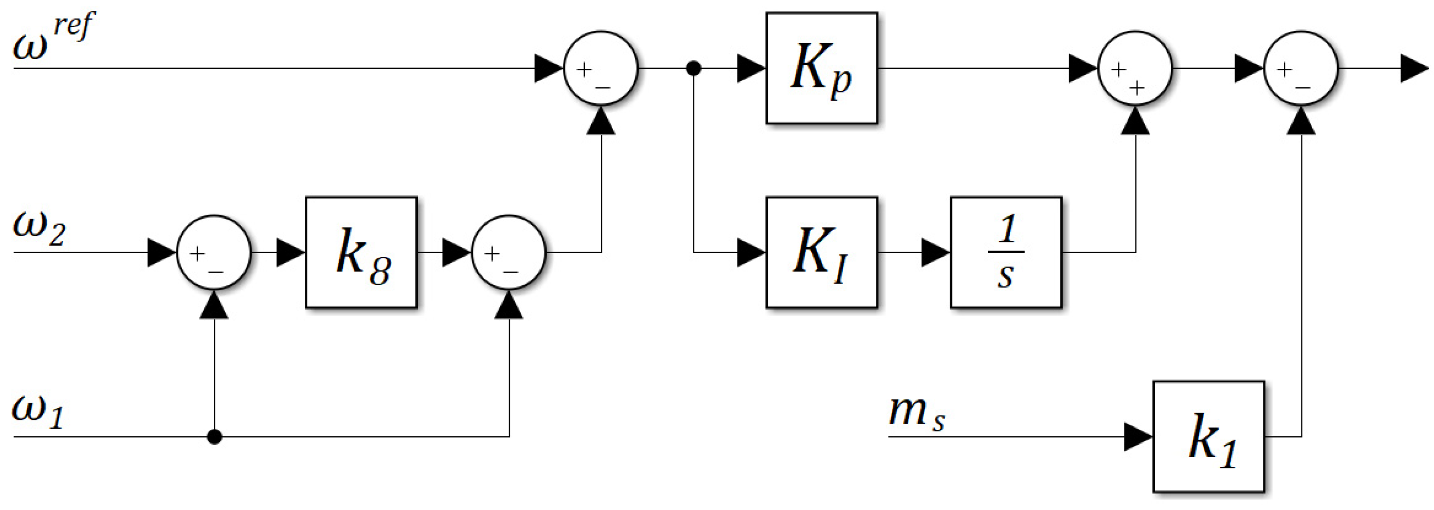
2.2. PI Controller with Additional Feedback Loops

One of the classical control structures assumes a PI controller with two additional feedbacks (from torsional torque and speed difference of the motor and load) [9]. The proposed structure is shown in Figure 1. It enables an arbitrary distribution of poles on the complex plane, which allows for wide shaping of the dynamics of the closed system.

According to the theory of modal control, in order to determine the controller settings and feedbacks, the characteristic polynomial of a closed system must be compared to a reference polynomial of the same order. By comparing the coefficients of said polynomials at particular levels, expressions describing the control system gains can be obtained:

$$k_8=\frac{1}{{\omega }_o{}^2{T}_1{T}_2{T}_c}-1,$$

(6)

$$k_1=\frac{T_1\left(4{\zeta }_o{}^2-k_8\right)}{T_2\left(1+k_8\right)},$$

(7)

$$K_P=4{\zeta }_o{\omega }_o{}^3{T}_1{T}_2{T}_c,$$

(8)

$$K_I={\omega }_o{}^4{T}_1{T}_2{T}_c,$$

(9)

where ${\omega }_o$—reference angular frequency, ${\zeta }_o$—set damping factor. The above relationships allow for the selection of gain coefficients for the analysed control system [9].

2.3. Predictive Control

Predictive control is based on determining a sequence of control signals that optimally minimises a given objective function on the so-called output prediction horizon. The number of calculated control signal values depends on the length of the control horizon. The future behaviour of the object is determined on the basis of the mathematical model. For this purpose, the model of the two-mass system (5) was expanded by two additional variables: load torque and reference speed. Their dynamics are dependent on individual applications and unknown from the point of view of the control structure. Hence, they are not taken into account when defining the mathematical model:

$$\frac{d}{dt}{m}_L=0,\frac{d}{dt}{\omega }^{ref}=0.$$

(10)

As a result, the drive state vector now consists of five elements:

$$X_c={\left[\begin{array}{ccccc}{\omega }_1& {\omega }_2& m_s& m_L& {\omega }^{ref}\end{array}\right]}^T.$$

(11)

The model described by Equation (5) which takes (10) into account was then discretised with a sampling time of $T_s$ using the Euler method. Additionally, to prevent the drive from damage, a constraint on electromagnetic and torsional torque in relation to the nominal electromagnetic torque level was introduced:

$$\begin{gathered} \left|m_e\right|\le 3\left(p.u.\right), \\ \left|m_s\right|\le 1.5\left(p.u.\right). \end{gathered}$$

(12)

The minimised outputs of the predictive controllers were declared as:

$$\begin{gathered} y_1={\omega }_1-{\omega }^{ref}, \\ {y}_2={\omega }_2-{\omega }^{ref}, \\ {y}_3=m_s-m_L. \end{gathered}$$

(13)

The first two outputs are responsible for minimising the difference between the speed of the drive motor and load machine and the reference speed. The third output allows for the minimisation of the difference between torsional and load torque. Ultimately the task of determining the optimal controls can be described by the equations:

$$\underset{u_1, u_2, \cdots ,u_{N_c-1}}{\min }\left\{{\displaystyle \sum }_{k=0}^N\left(q_1{\left(y_1\left(k\right)\right)}^2+q_2{\left(y_2\left(k\right)\right)}^2+q_3{\left(y_3\left(k\right)\right)}^2\right)+{\displaystyle \sum }_{j=1}^{N_c-1}r{\left(m_e\left(j\right)\right)}^2\right\},$$

(14)

$$\left|m_e\right|\le 3\left(p.u.\right),\left|m_s\right|\le 1.5\left(p.u.\right).$$

(15)

where $q_1$, $q_2$, $q_3$—weights differentiating the influence of the individual outputs on the control value, $r$—weight affecting the control damping, $N$—output prediction horizon, $N_c$—control prediction horizon.

The predictive control algorithm can be implemented in two ways. The traditional way is based on solving an on–line optimisation problem for a given state of the system $x\left(k\right)$ and the length of the prediction horizon adopted in the algorithm. It should be emphasised that increasing the prediction horizon length results in better dynamic properties of the object, but it also complicates the control algorithm significantly and thus increases the required computational effort. In practical solutions, very often a constant value of the control signal is assumed for the whole prediction horizon as a way of reducing the complexity of the entire algorithm. After determining the optimal value of the control signal at the time $k$, it is applied to the controlled object. In the next computational moment $\left(k+1\right)$ the whole procedure is repeated from the beginning, taking into account the current values of the object state vector $x\left(k+1\right)$, which can be either measured or estimated. The described control strategy requires the use of fast microprocessor systems.

When the required computational effort is too high, the explicit MPC control method is often used. In this case, the minimisation of the criterial function takes place off–line for all possible values of the state variables from the adopted range. For this purpose, the goal function is transformed into a multi–parametric quadratic programming problem whose solution is represented as a set of polyhedral regions in the state space. Replacing the traditional predictive controller with its explicit counterpart, a significant reduction of the required computational effort can be achieved.

In the following work, a fast gradient algorithm implemented in the C language [26] was used to minimise the objective function. Both the on-line and explicit control structure use information about the full state vector of the object, which is unmeasurable and therefore requires estimation. Two types of estimators were used in this study: the classic Luenberger observer and the Kalman filter.

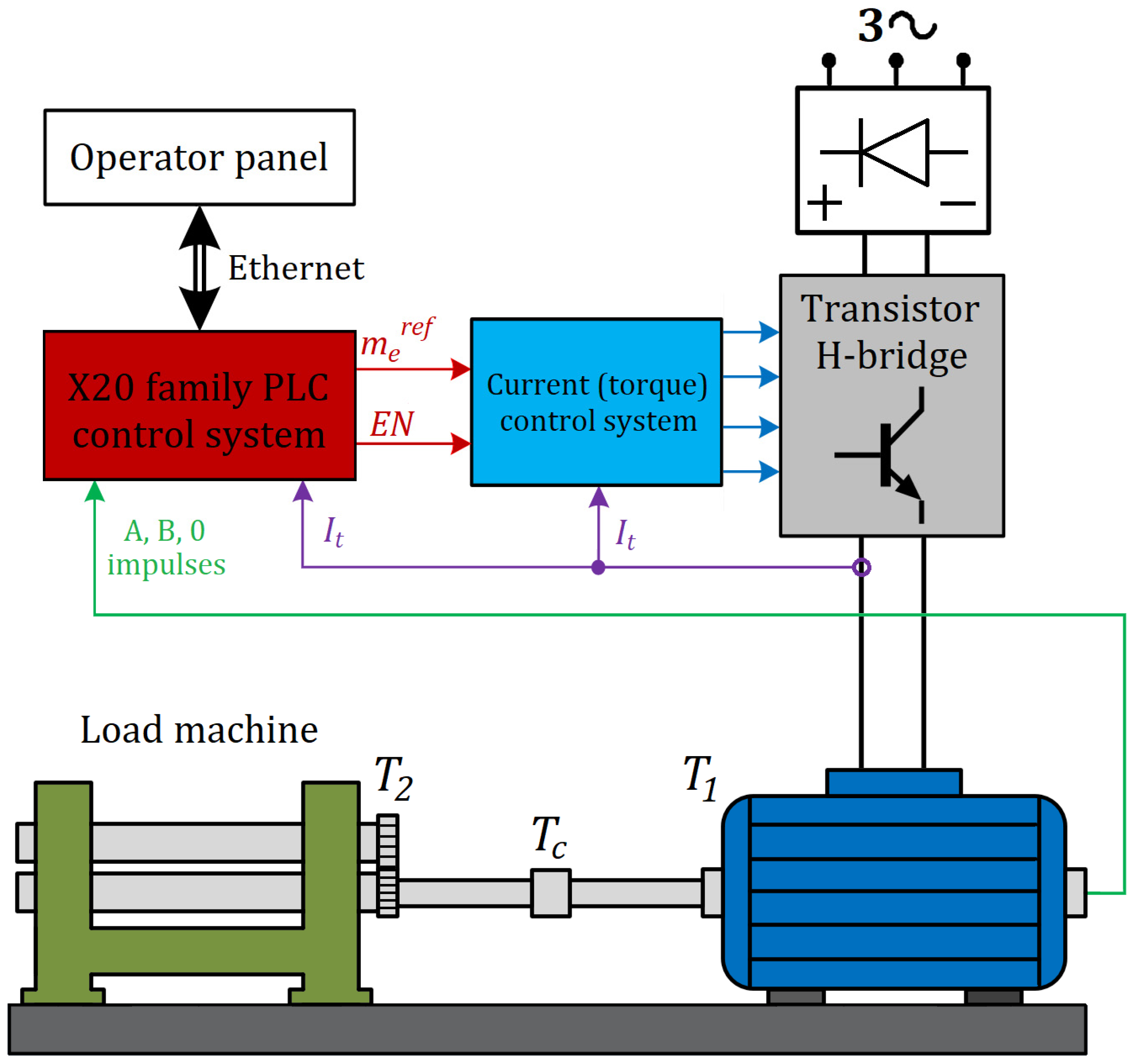
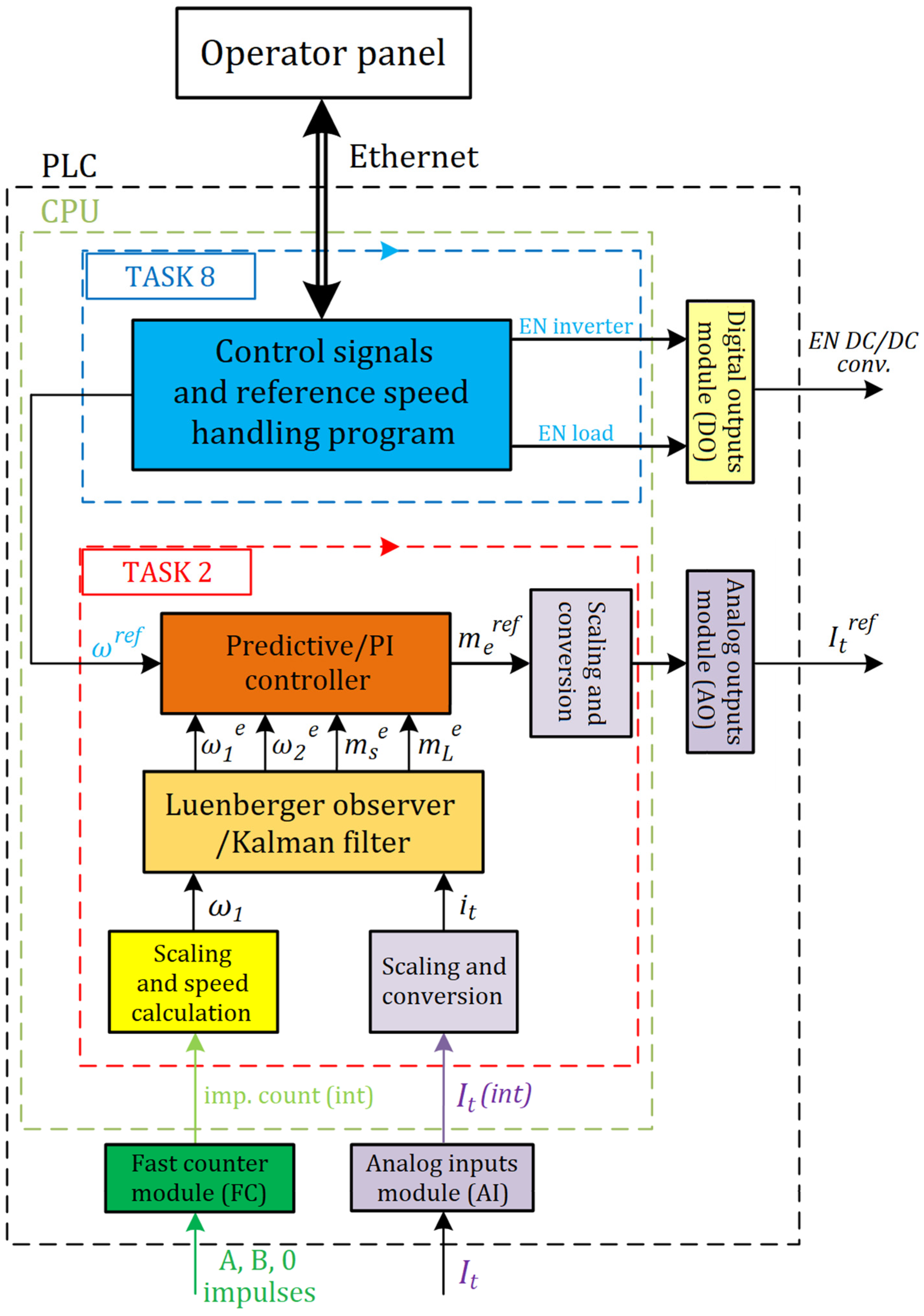
3. Implementation of the Control Structure

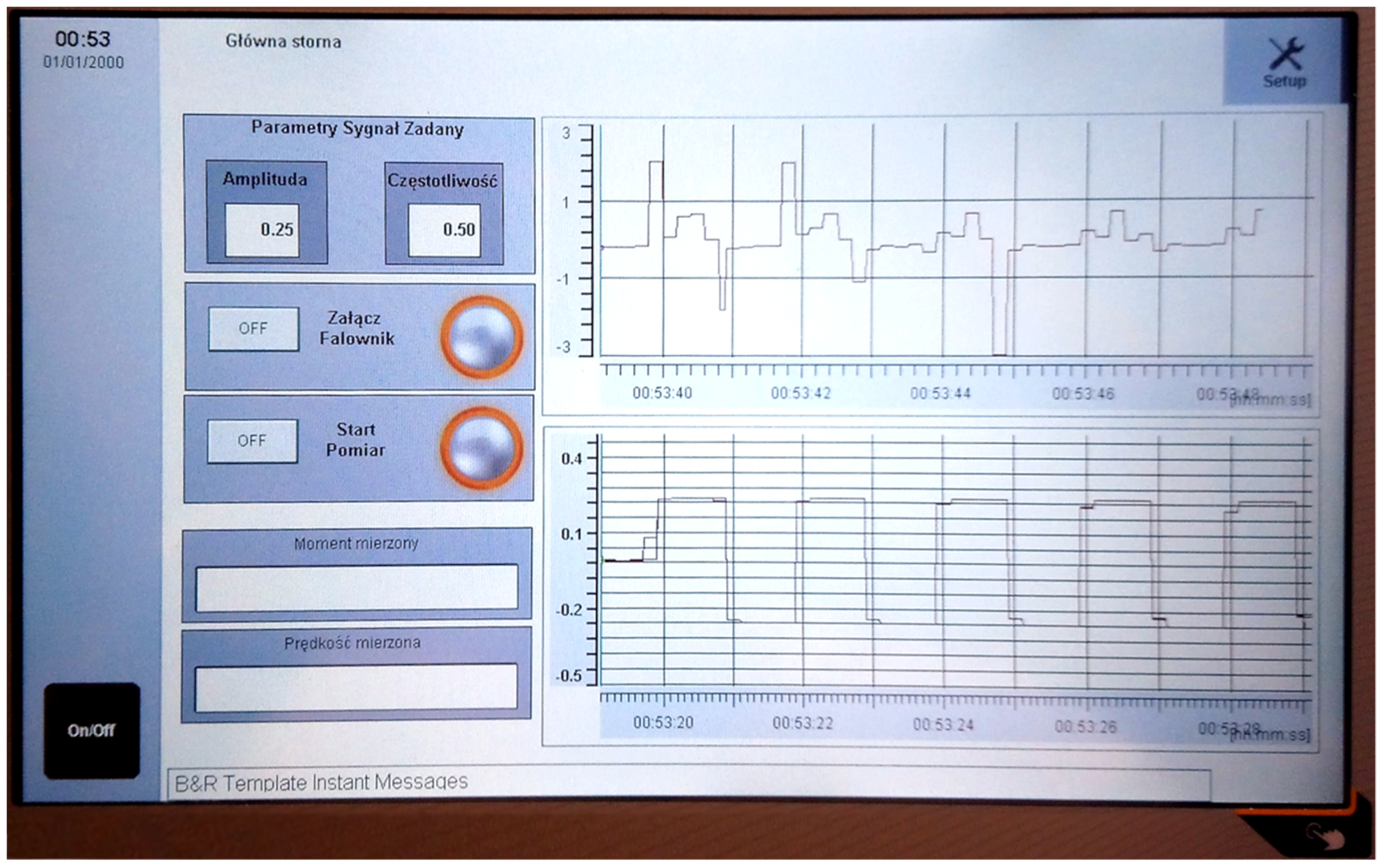
Figure 2 shows the proposed structure for industrial implementation. It is built of three main elements: the first one is the converter which enables control of the electromagnetic torque (current) of the drive. There are many companies which offer systems that enable such control. The second element is the programmable logic controller (PLC). In this study, a modular PLC of the X20 family from B&R [27] was used.

The controller consists of a CP3586 CPU, digital outputs module DO9322, analogue outputs module X20A04632, analogue inputs module AI4632 and a fast counter module adapted for incremental encoders DC1196. The basic parameters of the control system are presented in

Table 1. Parameters of the PLC used.

Description	Parameters
Central unit X20CP3586	INTEL ATOM 1.6 GHz processor, 512 MB DDR2 RAM, 1 MB SRAM, calculation speed up to 0.1 ms
Digital outputs X20DO9322	12 outputs, 24 VDC, 0.5 A
Analogue inputs X20AI4632	4 inputs ± 10 V/0 to 20 mA, 16 bit resolution, configurable input filter
Analogue outputs X20AO4632	4 outputs ± 10 V/0 to 20 mA, 16 bit resolution
High–speed counter X20DC1196	One ABR channel, 5 V, max frequency 600 kHz, 4 edges counted

.

In addition, the workstation is equipped with a 10” touch panel which can be used to operate and visualise the operation of the system. The third component is the drive built with two 500 W DC motors connected with a shaft of 5 mm diameter and 600 mm length. Parameters of the drive are presented in

Table A1. Parameters of drive.

Parameter	Symbol	Value
base pulsation	${\mathsf{\Omega }}_b$	151.84 rad/s
nominal speed	${\mathsf{\Omega }}_N$	1450 rev/min
rated current	$I_N$	3 A
rated (base) torque	$M_b$	3.15 Nm
nominal flux	${\mathsf{\Psi }}_N$	1.05 Wb
shaft spring constant	$K_c$	17.38 Nm/rad

. An encoder with a resolution of 36,000 imp/rev is installed on the drive motor.

In this work, Automation Studio (AS) software is used to configure and program all B&R components. It can be used to configure hardware as well as to write software. One of the additions to AS is an overlay that can be used to generate code from Simulink. The structure of the program is shown in Figure 3.

The program is divided into two main tasks. In the first one (called the Task 2 by B&R), the full control structure including the observer is implemented. This task is called every 1.2 ms. Adopting the above calculation step (task calling) is allowed because the total time constants of the object are much larger. In this case, sampling with such a step ensures adequate control quality. The Simulink library described earlier was used to create this part of the program. In the second task (called the Task 8 by B&R) there is a program related to handling of the visualisation generated on the operator panel and the control system of the converter and the drive load. This task is characterized by a relatively fast computation time (20 ms) and the lowest priority setting. The presented allocation of programmes in particular tasks makes the HMI system react quickly to the occurring signals, and at the same time its operation may be interrupted at any time by time-critical tasks (those which are related to control). The visualisation created is shown in Figure 4.

Since the speed was determined using the information from the fast counter, it had to be calculated on that basis. For this purpose, a simple calculation method which involves counting four slopes and scaling to relative units was used. Its implementation method is shown in Figure 5. For the measured current, it is only scaled and subjected to a type conversion from integer to a double precision floating point value.

4. Results

At first, hardware in the loop (HIL) tests were performed. The aim was to check how the designed control system (software part) would work on the PLC controller (data exchange between modules and the program via global and local variables). To enable simulation, a model of the two-mass drive was introduced to the first task, which was initially calculated with a step of 0.4 ms. A Luenberger observer was used in the controller as an estimator of the state variables. The parameters of the predictive controller and the observer are listed in

Table 2. Parameters of the predictive controller.

Parameter	Value
$T_s$	1.2 ms
$N$	12
$N_c$	2
$q$	$q_1=5;q_2=5;q_3=1$
$r$	0.001
$m_e{}^{max} \left(i_t{}^{max}\right)$	3 p.u.
$m_s{}^{max}$	1.5 p.u.

. The test consisted of cyclic turns with a pre-set speed of 0.25 and frequency of 0.5 Hz. The results of the system operation are presented in Figure 6.

As can be seen, the system experiences significant speed oscillations and rapid changes in electromagnetic torque. Under the assumed simulation conditions, the drive operates without any load in the start-up state. However, the obtained results show significant fluctuations of the estimated value of the load torque (Figure 6c). Such a large estimation error may cause unstable operation of the entire drive.

In the system, there are long delays between the generation of the reference signal and the response of the executive system. They are presented in more detail in Figure 7. In the case of a change of the reference signal, it is transferred to the executive system with a delay of two samples, after which the external torque (current) control system starts to react. This delay is related to the processing of global and local variables between different threads of the program. Due to the poor quality of the estimation, the Luenberger observer was replaced in further studies by a linear Kalman filter.

The subsequent step was to test how the parameters of the predictive controller affect the load on the CPU of the PLC controller. Two values of the output prediction horizon (12 and 25 samples) and two reference speed values (0.25 and 0.5) taken into account. It was also examined how the load on the CPU is affected by the use of the classic PI regulator. The results are presented in

Table 3. Comparison of program execution times by the PLC controller.

Parameter	CPU Usage (%)	Calculation Time (µs)
		Min	Average	Max
PI	3.5	36	42	93
$\mathrm{MPC}N=12,$ ${\omega }^{ref}=0.25$	4.8	165	188	197
$\mathrm{MPC}N=12,$ ${\omega }^{ref}=0.5$	6.5	177	192	199
$\mathrm{MPC}N=25,$ ${\omega }^{ref}=0.25$	5.2	178	192	198
$\mathrm{MPC}N=25,$ ${\omega }^{ref}=0.5$	8.5	230	251	263

.

The presented data shows that the predictive controller, even with a long output prediction horizon, does not overload the controller in a way that would make its operation impossible. The calculation time in the worst case is still less than 22% of the computation cycle of the entire program (stored in the task with a calculation time of 1.2 ms). However, compared to a PI controller with additional feedbacks, a significant increase in computation time and CPU load can be seen.

In the next step, the influence of weight factors on the dynamic properties of the drive was examined. The results for three sets of weights are shown in Figure 8.

It can be seen that as the weights of the objective functions related to the control error increase, the response rate also increases. The dynamic of the response is limited by the torsional torque constraint. Selecting greater weight values leads to a faster response to disturbances (load torque) but this can result in unstable operation (noise tracking).

Afterwards, the two considered control structures were tested experimentally on the setup shown in Figure 9, at a reference speed of 0.5. The predictive controller was tuned according to the parameters shown in Table 2, while the PI controller was tuned for a reference angular frequency of 60 rad/s and a damping ratio of 0.75. The results of this test are shown in Figure 10.

It can be observed that both control structures provide correct operation of the drive in steady state and good dynamic speed characteristics of both machines. However, during reversals the PI controller did not ensure the stabilisation of torsional torque below the set limit, which can lead to permanent damage to the shaft and failure of the entire drive system.

Finally, a function block was created from the predictive control structure, which was used to build a program in ladder diagram (LD) language. This program is shown in Figure 11, while Figure 12 shows the results obtained for selected state variables that were recorded with the dedicated analysis tool. As can be noticed, the drive system operates accurately—the load speed is achieved without oscillations and the torsional torque amplitude is maintained in a safe area.

5. Conclusions

In this paper issues related to the implementation of selected control structures of drives with elastic coupling on a PLC controller were considered. From the presented results it can be concluded that:

• It is possible to successfully implement an advanced control structure, such as a predictive controller with a Kalman filter, for drives with an elastic connections using a PLC controller;
• Even with a long prediction horizon of the outputs, which greatly increases the computational complexity of the controller, the computation time and CPU load of the PLC controller are sufficiently low;
• For the considered control system, the application of the linear Kalman filter provides a significant improvement in the estimation of state variables compared to a Luenberger observer;
• The presented solution allows for creation of a control function block, which can then be used in other projects as a component of control programs, saving time in the design process.

Future work could focus on implementing the presented structure for a PMSM servo drive, where the reference torque signal is transmitted via a POWERLINK network and the MotionControl standard is used. Another issue worth considering is to analyse the application possibilities for systems with higher resonant frequencies.

References

1. Zawirski, K.; Deskur, J.; Kaczmarek, T. Automatyka Napędu Elektrycznego; Wydawnictwo Politechniki Poznańskiej: Poznań, Poland, 2012. (In Polish) [Google Scholar]
2. Zhang, R.; Tong, C. Torsional vibration control of the main drive system of a rolling mill based on an extended state observer and linear quadratic control. J. Vib. Control 2006, 12, 313–327. [Google Scholar] [CrossRef]
3. Valenzuela, M.A.; Bentley, J.M.; Lorenz, R.D. Computer-aided controller setting procedure for paper machine drive systems. IEEE Trans. Ind. Electron. 2009, 45, 638–650. [Google Scholar] [CrossRef]
4. Luca, A.D.; Book, W. Robots with flexible elements. In Springer Handbook of Robotics; Springer: Berlin/Heidelberg, Germany, 2008; pp. 287–319. [Google Scholar] [CrossRef]
5. Štimac, G.; Braut, S.; Bulić, N.; Žigulić, R. Modeling and experimental verification of a flexible rotor/AMB system. COMPEL Int. J. Comput. Math. Electr. Electron. Eng. 2013, 32, 1244–1254. [Google Scholar] [CrossRef]
6. Montague, R.; Bingham, C.; Atallah, K. Servo control of magnetic gears. IEEE/ASME Trans. Mechatron. 2012, 17, 269–278. [Google Scholar] [CrossRef]
7. Łuczak, D. The Use of Digital Filters in Control Systems of Electric Drives with Complex Mechanical Structure; Poznań University of Technology: Poznań, Poland, 2014. [Google Scholar]
8. Muszyński, R.; Deskur, J. Damping of torsional vibrations in high-dynamic industrial drives. IEEE Trans. Ind. Electron. 2009, 57, 544–552. [Google Scholar] [CrossRef]
9. Szabat, K.; Orłowska-Kowalska, T. Vibration suppression in a two-mass drive system using PI speed controller and additional feedbacks—Comparative study. IEEE Trans. Ind. Electron. 2007, 54, 1193–1206. [Google Scholar] [CrossRef]
10. Kabziński, J.; Mosiołek, P. Integrated, multi-approach, adaptive control of two-mass drive with nonlinear damping and stiffness. Energies 2021, 14, 5475. [Google Scholar] [CrossRef]
11. Petit, F.; Daasch, A.; Albu-Schäffer, A. Backstepping control of variable stiffness robots. IEEE Trans. Control Syst. Technol. 2015, 23, 2195–2202. [Google Scholar] [CrossRef]
12. Kamiński, M.; Szabat, K. Adaptive control structure with neural data processing applied for electrical drive with elastic shaft. Energies 2021, 14, 3389. [Google Scholar] [CrossRef]
13. Wróbel, K.; Serkies, P.; Szabat, K. Model predictive base direct speed control of induction motor drive—Continuous and finite set approaches. Energies 2020, 13, 1193. [Google Scholar] [CrossRef] [Green Version]
14. Wang, C.; Yang, M.; Zheng, W.; Long, J.; Xu, D. Vibration suppression with shaft torque limitation using explicit MPC-PI switching control in elastic drive systems. IEEE Trans. Ind. Electron. 2015, 62, 6855–6867. [Google Scholar] [CrossRef]
15. Cychowski, M.; Szabat, K.; Orłowska-Kowalska, T. Constrained model predictive control of the drive system with mechanical elasticity. IEEE Trans. Ind. Electron. 2009, 56, 1963–1973. [Google Scholar] [CrossRef]
16. Serkies, P.; Szabat, K. Application of the MPC controller to the position control of the two-mass drive system. IEEE Trans. Ind. Electron. 2013, 60, 3679–3688. [Google Scholar] [CrossRef]
17. Vittek, J.; Ryvkin, S. Decomposed sliding mode control of the drive with interior permanent magnet synchronous motor and flexible coupling. Math. Probl. Eng. 2013, 2013, 680376. [Google Scholar] [CrossRef] [Green Version]
18. Serkies, P.; Szabat, K. Effective damping of the torsional vibrations of the drive system with an elastic joint based on the forced dynamic control algorithms. J. Vib. Control 2019, 25, 2225–2236. [Google Scholar] [CrossRef]
19. Ilchmann, A.; Schuster, H. PI-funnel control for two mass systems. IEEE Trans. Autom. Control 2009, 54, 918–923. [Google Scholar] [CrossRef] [Green Version]
20. Vouzis, P.D.; Bleris, L.G.; Arnold, M.G.; Kothare, M.V. A system-on-a-chip implementation for embedded real-time model predictive control. IEEE Trans. Control Syst. Technol. 2009, 17, 1006–1017. [Google Scholar] [CrossRef]
21. Jerez, J.L.; Goulart, P.J.; Richter, S.; Constantinides, G.A.; Kerrigan, E.C.; Morari, M. Embedded predictive control of an FPGA using the fast gradient method. In Proceedings of the European Control Conference (EEC), Zürich, Switzerland, 17–19 July 2013. [Google Scholar] [CrossRef]
22. Dominic, S.; Löhr, Y.; Schwung, A.; Ding, S.X. PLC-based real-time realization of flatness-based feedforward control for industrial compression systems. IEEE Trans. Ind. Electron. 2017, 64, 1323–1331. [Google Scholar] [CrossRef]
23. Aboelhassan, A.; Abdelgeliel, M.; Zakzouk, E.E.; Galea, M. Design and implementation of model predictive control based PID controller for industrial applications. Energies 2020, 13, 6594. [Google Scholar] [CrossRef]
24. Valencia-Palomo, G.; Rossiter, J.A. Efficient suboptimal parametric solutions to predictive control for PLC applications. Control Eng. Pract. 2011, 19, 732–743. [Google Scholar] [CrossRef] [Green Version]
25. Lozynskyy, A.; Chaban, A.; Perzyński, T.; Szafraniec, A.; Kasha, L. Application of fractional-order calculus to improve the mathematical model of a two-mass system with a long shaft. Energies 2021, 14, 1854. [Google Scholar] [CrossRef]
26. MathWorks. Model Predictive Control Toolbox™. Available online: https://www.mathworks.com/products/model-predictive-control.html (accessed on 1 December 2021).
27. B&R Automation. Available online: https://www.br-automation.com/en-gb/products/plc-systems/x20-system/x20-cpus/x20cp3586/ (accessed on 26 November 2021).
Figure 1. PI controller structure with two additional feedbacks.
Electronics 10 03139 g001
Figure 2. Proposed structure for industrial implementation.
Electronics 10 03139 g002
Figure 3. Structure of the program.
Electronics 10 03139 g003
Figure 4. Operator panel with visualisation.
Electronics 10 03139 g004
Figure 5. Speed calculation algorithm.
Electronics 10 03139 g005
Figure 6. The results of a HIL simulation with Luenberger observer: (a) Drive motor speed, (b) load speed, (c) torsional and load torque.
Electronics 10 03139 g006
Figure 7. Response delay of the torque control system.
Electronics 10 03139 g007
Figure 8. Impact of objective function weights on the dynamic properties of the system: (a,c) torque, (b,d) speed.
Electronics 10 03139 g008
Figure 9. Full view of the experimental setup.
Electronics 10 03139 g009
Figure 10. Comparison between PI (a,b) and predictive (c,d) controllers: (a) torque, (b) speed.
Electronics 10 03139 g010
Figure 11. Created function block.
Electronics 10 03139 g011
Figure 12. Operation of the applied function block: (a) torsional torque, (b) load speed.
Electronics 10 03139 g012