A Method for Class-Imbalance Learning in Android Malware Detection

Abstract

More and more Android application developers are adopting many different methods against reverse engineering, such as adding a shell, resulting in certain features that cannot be obtained through decompilation, which causes a serious sample imbalance in Android malware detection based on machine learning. Hence, the researchers have focused on how to solve class-imbalance to improve the performance of Android malware detection. However, the disadvantages of the existing class-imbalance learning are mainly the loss of valuable samples and the computational cost. In this paper, we propose a method of Class-Imbalance Learning (CIL), which first selects representative features, uses the clustering K-Means algorithm and under-sampling to retain the important samples of the majority class while reducing the number of samples of the majority class. After that, we use the Synthetic Minority Over-Sampling Technique (SMOTE) algorithm to generate minority class samples for data balance, and finally use the Random Forest (RF) algorithm to build a malware detection model. The result of experiments indicates that CIL effectively improves the performance of Android malware detection based on machine learning, especially for class imbalance. Compared with existing class-imbalance learning methods, CIL is also effective for the Machine Learning Repository from the University of California, Irvine (UCI) and has better performance in some data sets.

1. Introduction

Because it is open source, the Android system has always been at the top in terms of market share. According to an IDC report, the market share of the Android system reached 84.1% in 2020 [1]. Therefore, the number of Android applications is considerable. Correspondingly, Android malware is also flooding the third-party application market, bringing unprecedented challenges to information security [2,3,4]. At present, researchers mainly adopt static and dynamic methods to analyze Android malware. Both method types have their own advantages and disadvantages [5,6,7]. In view of the large number of applications, machine learning is adopted by many researchers, and unlike when checking the signature of the applications, unknown applications can be detected [2]. Generally, a balanced training set is beneficial for machine learning, but in reality, unbalanced training sets are common [8]. If a certain type in a data set exceeds 65%, it is considered an unbalanced data set; examples include credit card data, or the diagnosis of cancer patients [9,10]. For an unbalanced data set, the result will be biased towards the majority class [11,12]. Now, for Android malware detection, developers protect their applications by packing so that others cannot obtain the source code of the application [13,14]. This also increases the difficulty of Android malware detection based on machine learning, because the Android application features are mainly derived from the decompiled source code. Hence, one can obtain information regarding permissions and components from the AndroidManifest.xml, but it is not possible to obtain the fine-grained API features [15]. In addition, as the difference in permissions between malware and benign apps becomes smaller and smaller, it is hard to give better results if only the permissions are used as the features.

Taking the Xiaomi application market as an example, randomly downloaded apps are all packed. This means that using the apktool tool to acquire the source code is unsuccessful, while most of the apps from public malware databases such as VirusShare [16] can be successfully reversed, which results in a huge disparity in the ratio of the majority and minority classes when using the API features. Therefore, the number of malicious apps is much larger than that of benign apps in the data set. Traditional machine learning algorithms cannot fully learn the minority class, so the results are biased to the majority class; it may be that the minority class samples cannot be detected at all. Many methods have been designed to solve class imbalance, mainly from data processing, algorithm, and feature selection [17,18,19]. In these methods, the under-sampling and over-sampling methods are most often used. The under-sampling technique randomly reduces the number of samples in the majority class to achieve a balance, but the most important samples may be lost [20]. The over-sampling technique is opposite to the under-sampling technique: it achieves a balance of positive and negative samples by adding samples to the minority class. Although it meets the requirements of obtaining greater balance, it is prone to overfitting [21]. More details about these methods are presented in Section 2.

In view of the complementarity of the under-sampling and over-sampling techniques, the method proposed in this paper is inspired by the BalanceCascade algorithm. First, the clustering K-Means algorithm [22] is used to cluster majority-class samples, and the samples for training are selected proportionally in each cluster to ensure the diversity of malicious apps. Secondly, malicious apps were randomly selected from the different clusters, equal to the number of benign apps, to establish an Android malware detection model; all the majority-class samples were tested to remove the samples with the correct classification, and then samples were selected from the remaining majority-class samples to establish a new detection model to further reduce the number of majority-class samples. This was iterated until the number of undetected malicious apps (i.e., majority class samples) was less than or equal to the number of benign apps, and these malicious apps were kept together with the previous malicious apps involved in the detection model. Finally, the SMOTE algorithm was used to generate the minority class samples for balance, and the RF algorithm was applied to learn the training set to detect unknown applications.

The significant contributions of the paper include the following aspects:

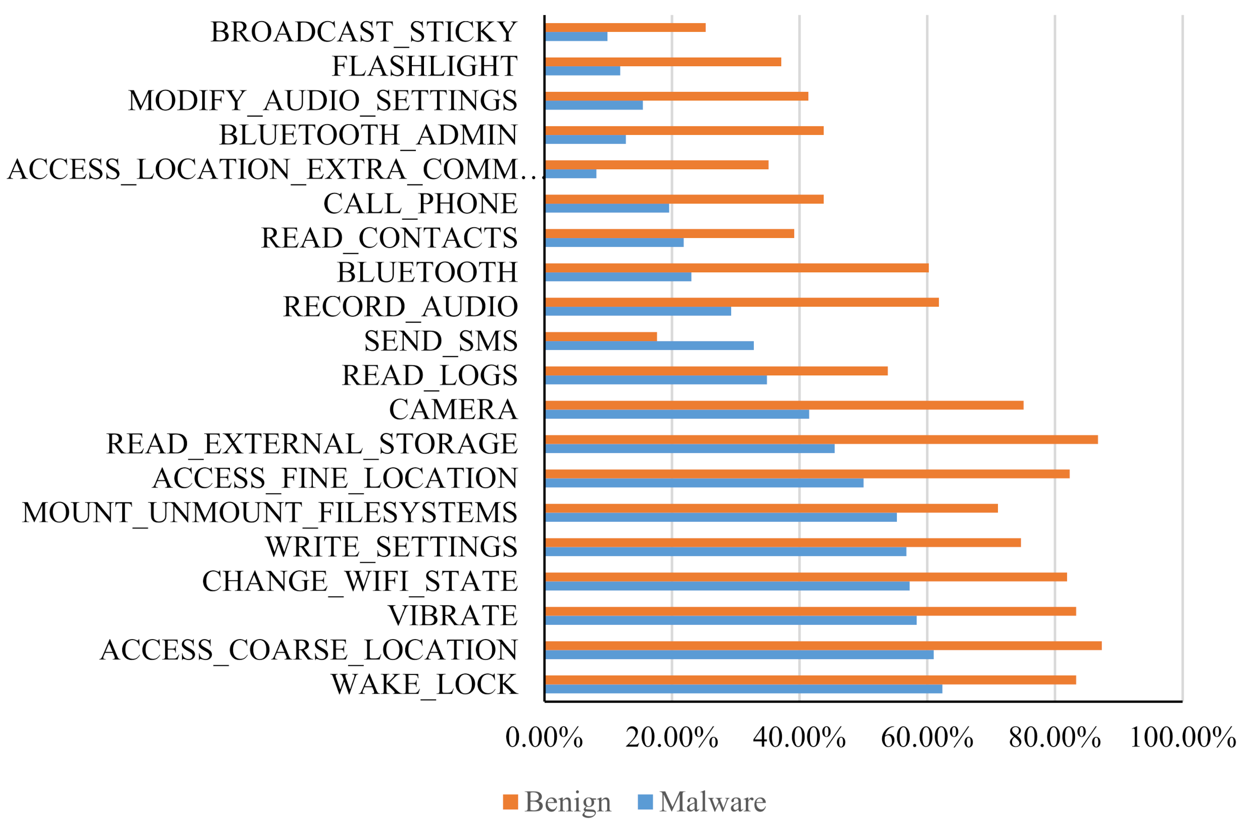
• According to the usage frequency of the same permissions and APIs in benign apps and malware, we selected the features, which represent the difference between malware and benign apps and improve the performance of Android malware detection.
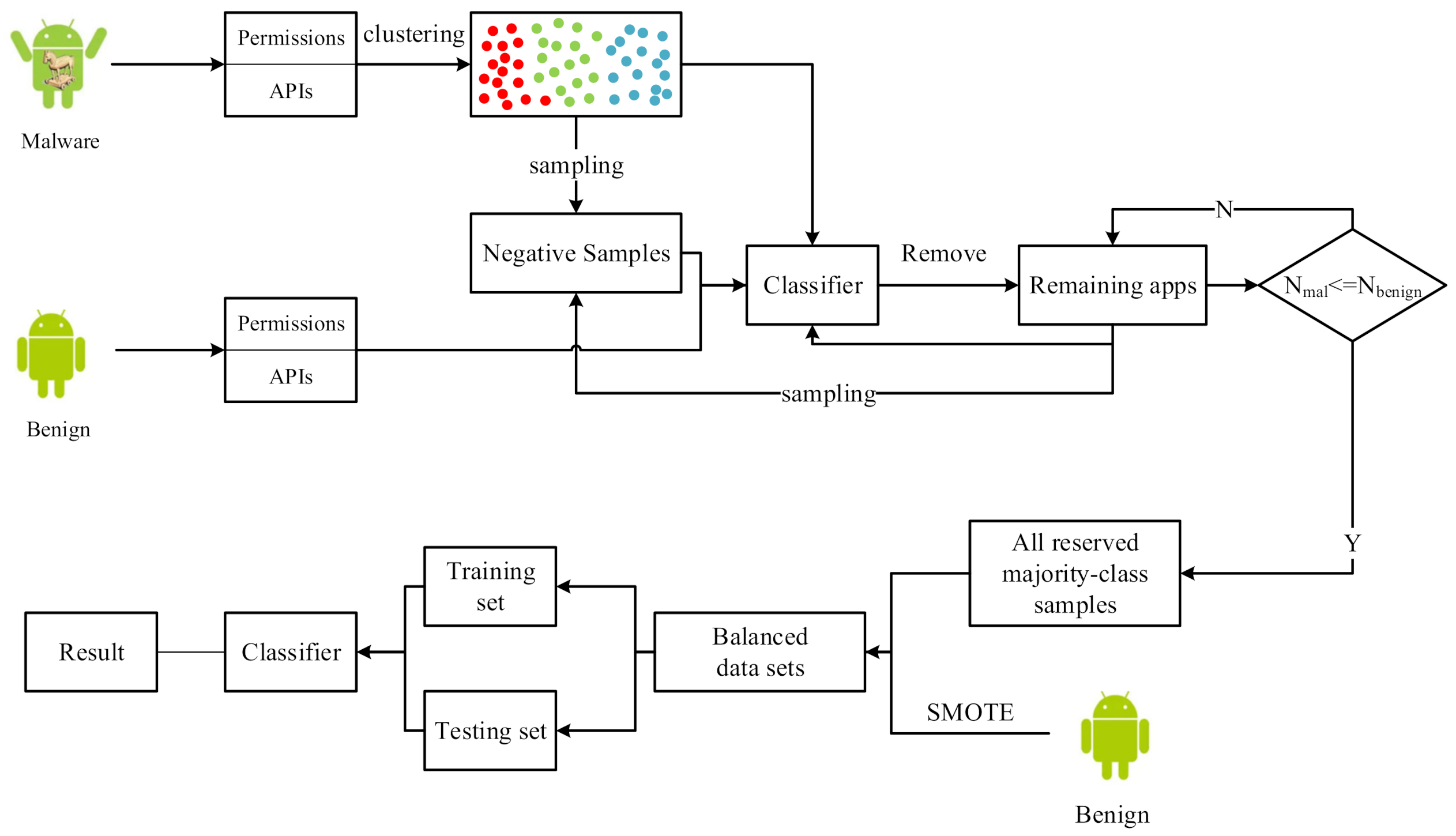
• CIL takes the advantage of the clustering algorithm, under-sampling, and over-sampling. In the process of under-sampling, it focuses on learning malware from different clusters that are not correctly classified to avoid losing important samples and reduce the number of malicious apps. Then, over-sampling is used to generate minority-class samples to construct a balanced training set to improve the performance of the classifier and mitigate the effect of over-fitting. Furthermore, the reduction in the number of training samples helps save the time overhead for machine learning.
• CIL is suitable not only for solving the problem of class imbalance in the field of Android malware detection, but also for unbalanced data sets from UCI. It demonstrates that CIL has generalization capability.

The rest of this paper is organized as follows: Section 2 reviews the background of this paper; Section 3 presents our proposed method; Section 4 reports the results of our experiment; and finally, Section 5 concludes this paper.

2. Background

2.1. Feature Extraction and Selection

Feature selection applied in imbalanced data is mainly used to select features that are conducive to improving the performance of the classifier, used herein to clearly reflect the difference between benign and malware samples. There are many Android application features for machine learning, and the choice of features is crucial [18]. In the literature [23], feature selection was combined with the KNN algorithm, which significantly improved the performance of the classification algorithm on imbalanced data. MGRFE [24] reduces the number of features through feature selection and improves the classification accuracy of imbalanced data sets. Since dynamically acquiring features is very time-consuming, CIL uses a static method to select two types of features commonly used in most research: one is the permissions that the apps apply, and the other is the APIs called in the apps. The permission mechanism is an important measure for the Android system to protect users’ private information. The application cannot call the APIs protected by the permissions without authorization [25]. However, just using the permissions to detect malware is not enough. Especially with the evolution of malicious apps, the difference in permissions between malware and benign apps is diminishing. The 1200 malware apps collected around 2012 applied for an average of 13 permissions, while the malware collected in 2016 by VirusShare applied for an average of 33 permissions. In addition, 1000 benign apps that were recently randomly downloaded from App Market applied for an average of 36 permissions. This number of permissions is close to that of malicious apps in 2016 and significantly more than that of malicious apps collected in 2012. The difference in the number of permissions directly affects the detection effect of machine learning. The result of using only malicious apps from 2012 and benign apps as the training set is significantly better than that using the combination of malicious apps provided by VirusShare and the same benign apps. For this paper, we selected malicious apps from VirusShare as the sample and chose the permissions depending on the ratio of malicious and benign applications for the same feature, which represents the difference between the malware and benign apps.

Besides this, the execution of application behaviors must invoke APIs for implementation. Compared with permission features, the API features are more fine-grained. There are tens of thousands of APIs for selection. In order to reduce the number of API features, in this paper we only extracted the APIs under the android, java, and Javax packages from malicious and benign apps as features. Finally, 129 APIs with significant differences in benign and malicious apps were selected as features.

2.2. Related Work

In Section 2.1, the importance of feature selection was explained. Now, we present the details of the data preprocessing and algorithm. Generally, researchers define the minority-class samples of interest as the positive class and the majority-class samples as the negative class. The data processing method achieves a balance in the number of positive and negative samples through under-sampling, over-sampling, and mixed sampling. In order to avoid the loss of important samples by under-sampling, the extraction of valuable samples has become the focus of under-sampling research, such as the EasyEnsemble and BalanceCascade algorithms [26]. The BalanceCascade algorithm combines data preprocessing and ensemble algorithms. The majority class sample is defined as N, and the minority class is defined as P. Each time a set the same size as P is randomly selected from N, a balanced data set is used for learning using the Adaboost algorithm. By adjusting the threshold of the classifier, the misjudgment rate of the classifier is guaranteed to be f. Then the classifier classifies the majority-class samples and removes the correctly classified samples. It extracts a majority of samples equal in number to P from the remaining majority-class samples, and performs learning again until the iteration stops. However, when dealing with a large data sets, the computation cost is quite severe [27]. UFFDFR [28] uses a denoising stage to reduce the effect of noise samples and fuzzy c-means clustering algorithm to improve the performance of classification, and selects the representative samples based on distance. The three parts of UFFDFR are in sequence, so any unsatisfactory part will affect the final result. For over-sampling, only minority samples are randomly copied at first, but the over-fitting is serious. The SMOTE algorithm is the most widely used by researchers as the over-sampling method. It does not simply copy but analyzes minority-class samples to generate new samples and add them to the data set. The generated minority-class samples by SMOTE has a similar region with majority-class samples, which causing difficulty in classification [29]. Borderline SMOTE [30] improves on the basis of SMOTE by dividing the data into three categories and only over-sampling a few of the dangerous categories to improve the distribution of samples. However, it only gives more attention to the danger minority-class samples. ADASYN (Adaptive Synthetic Sampling) [31] assigns different weights to minority samples and generates new samples based on the weights. Hence, it is easily to be affected by outliers. In order to overcome the shortcomings of over-sampling and under-sampling, some researchers have adopted hybrid algorithms that combine over-sampling and under-sampling techniques. The authors of [32] first removed the noise in the data set, then obtained the majority class and the minority class through clustering, using under-sampling to remove the majority class samples, and used the SMOTE algorithm to generate so-called intelligent samples to balance the data set. Evolutionary Hybrid Sampling technique (EHSO) first determines the overlap area of the positive and negative classes, and then uses the SMOTE algorithm to copy the minority-class samples in the area where the positive and negative samples overlap, so as to avoid generating approximate samples for difficult-to-classify samples. The selection of the optimal K in KNN algorithm is still need to be further studied [33].

Choosing an appropriate algorithm is also important to solving sample imbalance. Among such algorithms, ensemble learning is widely used; it can reduce overfitting, and the effect is better than that of a single classifier. Adaboost is a boosting method. Although it is not specifically used for unbalanced data set processing, through iteration, the wrongly classified samples are given more weight, so that a minority of samples are given higher weights, including EasyEnsemble and BalanceCascade algorithms, RUSboost [34], and so on, taking Adaboost as the algorithm. The random forest algorithm based on multiple decision tree classifiers is also an ensemble algorithm that combines the Bagging and random subspace algorithms. The classification results are determined by the decision tree voting [35,36]. Unlike the Bagging algorithm, it randomly extracts some features each time, the data set adopts the self-service resampling technique (Bootstrap), and the randomly selected samples are used as the training set [37]. Therefore, the random forest algorithm can avoid overfitting. When training on an unbalanced data set, the algorithm can balance errors. In addition, researchers have also used single classification algorithms to solve the problem of class imbalance, such as one-class SVM, which treats samples of the minority class as novel points, learns the samples of the majority class, and detects so-called novel points [38].

In our experiment, the clustering algorithm was applied to the majority-class samples. Therefore, we simply introduce the K-means algorithm. The K-means algorithm is a partition-based clustering algorithm that performs unsupervised learning and is one of the top ten classic data mining algorithms. The idea of the algorithm is to cluster K-many points in the space as centers and classify the objects closest to the centers. Through an iterative method, the arrival of each cluster center is gradually updated until the best clustering result is obtained. It is used to measure the similarity of objects in the same cluster and the similarity of objects in different clusters. The key of the K-means algorithm is to select the appropriate K value. In this paper, we used the elbow method to determine the optimal K value, which is a good indication that the underlying model fits best at the chosen K.

3. The Proposed Method

In order to retains valuable samples from the majority class and controls the size of the training set, we proposed a method of class-imbalance learning with feature selection, clustering-based under-sampling and the SMOTE algorithm to generate new minority-class samples, called CIL. The architecture of CIL is as shown in Figure 1.

First, we selected representative features based on the utilization rate of the same feature in benign and malicious apps. We extracted the permissions and APIs from malware and benign apps, and we used Equations (1) and (2) to calculate the frequency of the features used:

$$f_i=\left\{\begin{array}{c}1 if the feature in the app\\ 0 otherwises \end{array}\right.$$

(1)

$$R\left(f\right)=|\frac{{\sum }_{i=1}^n{f}_i}{n}-\frac{{\sum }_{j=1}^m{f}_j}{m}|$$

(2)

where $R\left(f\right)$ represents the difference between the rate of feature used in malware and that in benign apps, n represents the size of the malware data set, and m represents the size of the benign app data set.

There are many kinds of Android malware families, and each family has its own characteristics that are different from the others. Therefore, we used the clustering algorithm K-Means to cluster the majority-class samples. Because K-means algorithm is one part of our proposed method, it is very important to choose an optimal K value. In this paper, the elbow method was used to determine the optimal K, which is the most well-known method for determining the optimal number of clusters. We extract samples according to the proportions of samples in different clusters. The total number of selected majority-class samples was equal to the number of minority-class samples, and they were used as the training set together. The RF algorithm was used to train the classifier. Then, all the majority-class samples were used as the test set. After test, we removed the majority-class samples that were correctly classified and preserved the majority-class samples involved in training set for the final model. We repeated the above process until the number of samples in the majority class that was not correctly classified was less than or equal to the number of samples in the positive class.

Finally, we used the SMOTE algorithm to generate new minority-class samples to achieve balance. Additionally, we used the majority-class and minority-class samples as the training set for constructing the Android malware detection model. Algorithm 1 presents the pseudo-code of CIL.

Algorithm 1 Given: Data set, where the minority-class samples are P, and the majority-class samples are N

Do While $\left|P\right| < \left|N\right|$ Perform cluster analysis on the majority-class samples, and use a subset of the majority class $N_i$ according to the ratio of the numbers of samples from different clusters, and $\left|P\right| = \left|N_i\right|$. The training set is composed of $N_i$ and P, and the RF is applied to train classifier $H_i$. Use classifier $H_i$ to classify the majority-class samples, remove the samples correctly classified from N, and iterate n times until the number of majority-class samples is less than or equal to the number of minority-class samples. Take ${\cup }_{i=1}^n{N}_i$ and the rest of majority-class samples with P as the data sets, and use the SMOTE algorithm to generate new minority-class samples to achieve a balanced training set. Using the training set obtained in Step 4, RF is used to train the final model for Android malware detection.

4. Experiment

The experiments were implemented in Windows 8.1 OS with i7-4720HQ CPU @ 2.60 GHz and 16 G memory. All the algorithms were provided by Python sklearn package and the parameters were mainly the default values. All the detections were verified by 10-fold cross-validation.

4.1. Experimental Samples and Evaluation Indicators

The malicious samples selected in this article were taken from a total of 10,182 apps collected by VirusShare and only 127 benign apps, which were decompiled and validated by VirusTotal. The ratio of positive to negative samples was 1:80. Although this is a large number of malware apps, many of them belonged to the same malware family. After extracting features, there was a large number of repeated samples. After removing the duplicates, the ratio was reduced to 1:40.

The detection and evaluation indicators used in most studies mainly include Accuracy, Precision, Recall, F-measure, and AUC [39,40]. The AUC indicator refers to the area under the ROC curve. The larger the area, the better the performance of the classifier. However, for unbalanced data sets, Accuracy is not suitable as an evaluation indicator, because the minority class is the focus of the study [41]. The definitions of these metrics are listed as follows:

$$\mathrm{Accuracy}=\frac{TP+TN}{TP+FN+FP+TN}$$

(3)

$$\mathrm{Precision}=\frac{TP}{TP+FP}$$

(4)

$$\mathrm{Recall}=\frac{TP}{TP+FN}$$

(5)

$$\mathrm{F-measure}=\frac{({\alpha }^2+1)\mathrm{precision}\times \mathrm{Recall}}{{\alpha }^2(\mathrm{Precision}+\mathrm{Recall})}$$

(6)

where $TP$, is the test result that predicted benign apps classified correctly. $FP$ is the test result that the malware incorrectly predicted as benign apps. $TN$ is the test result that predicted malware classified correctly. $FN$ is the test result that wrongly classifies benign apps as malware.

4.2. The Result of Permissions and APIs as Features

In the field of Android malware detection, permissions and APIs are widely used the features of machine learning by researchers. According to the above method, we chose 20 requested permissions with obvious differences from more than 100 permissions, as shown in Figure 2, and representative APIs as features, totaling 129. We do not list the APIs because of space limitations.

The 20 permissions listed in Figure 2 were used as features, and the random forest, KNN, NB, and SVM algorithms were used for training. Although the permissions selected can reflect the difference between benign and malicious applications, the detection results of all classification algorithms were biased towards the majority class due to the obvious class imbalance. Therefore, when the positive and negative samples are severely unbalanced, permission-based detection cannot be applied. We chose 129 APIs as features, and still used the above algorithms. The detection results of the APIs as features were relatively better than those of permissions as features, mainly because APIs are more granular and the number of APIs far outweighed that of permissions. However, the detection results were still biased towards the majority class, and the effect was still not ideal.

Taking the permissions and APIs above together as features, the results are shown in

Table 1. Results for permissions and APIs used as features together.

	Ratio	Precision	Recall	F1
NB	1:10	0.268 ± 003	0.763 ± 007	0.395 ± 005
	1:20	0.145 ± 001	0.765 ± 008	0.244 ± 002
	1:30	0.100 ± 001	0.765 ± 007	0.178 ± 002
	1:40	0.079 ± 000	0.771 ± 004	0.144 ± 001
RF	1:10	0.795 ± 013	0.464 ± 014	0.576 ± 013
	1:20	0.737 ± 027	0.218 ± 014	0.317 ± 018
	1:30	0.657 ± 071	0.216 ± 016	0.316 ± 024
	1:40	0.631 ± 061	0.192 ± 011	0.286 ± 012
KNN	1:10	0.581 ± 014	0.615 ± 015	0.592 ± 012
	1:20	0.513 ± 027	0.551 ± 018	0.523 ± 018
	1:30	0.492 ± 015	0.461 ± 012	0.466 ± 014
	1:40	0.489 ± 022	0.381 ± 016	0.421 ± 011
SVM	1:10	0.787 ± 021	0.468 ± 010	0.574 ± 011
	1:20	0.685 ± 081	0.163 ± 020	0.254 ± 030
	1:30	0	0	0
	1:40	0	0	0

. From the results, it can be seen that when using permissions and APIs as features together, the algorithms took effect. However, class imbalance still had an impact. The results show that the Precision of the RF algorithm was the best with different proportions, but the Recall was poor. The Recall indicator of the NB algorithm was the best among the four algorithms, but the low Precision led to unsatisfactory F1. When the ratio of the sample was 1:30 or 1:40, the SVM algorithm failed to detect benign applications (i.e., minority-class samples), and the results were completely biased toward malicious applications. Considering the F1, KNN was the best among the four algorithms. In general, the greater the level of imbalance, the worse the effect, with even the possibility of complete failure.

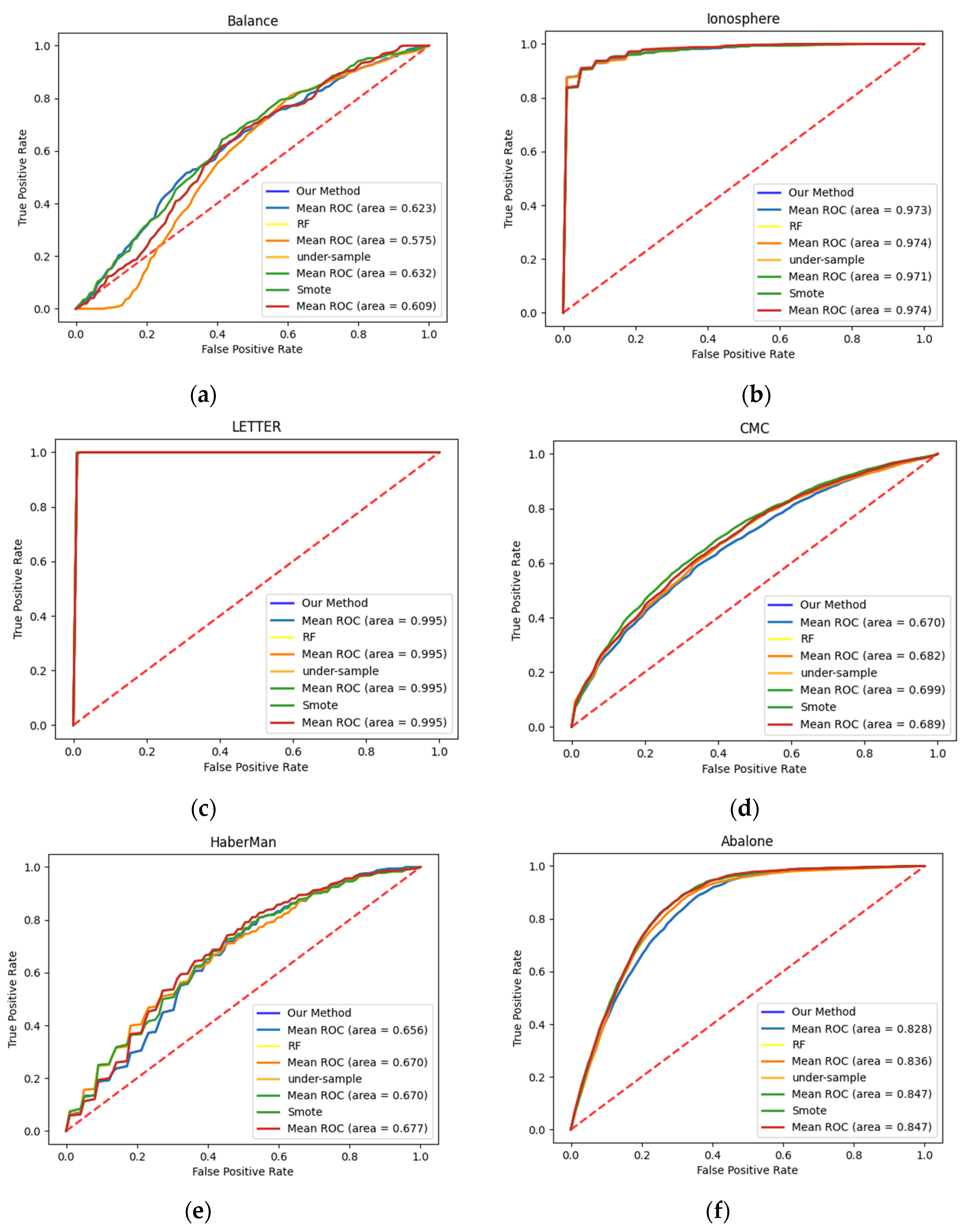
4.3. The Result of the Proposed Method

Data sets with different ratios were used to test the effectiveness of CIL. In the experiments, we determine the optimal K value based on the elbow method. The results are shown in

Table 2. Results of CIL.

	Ratio	Precision	Recall	F1
NB	1:10	0.310 ± 015	0.751 ± 015	0.434 ± 012
	1:20	0.161 ± 003	0.764 ± 009	0.265 ± 005
	1:30	0.109 ± 002	0.765 ± 008	0.191 ± 003
	1:40	0.087 ± 001	0.773 ± 006	0.157 ± 002
RF	1:10	0.758 ± 022	0.597 ± 020	0.655 ± 020
	1:20	0.700 ± 016	0.491 ± 004	0.565 ± 006
	1:30	0.677 ± 030	0.396 ± 016	0.485 ± 014
	1:40	0.671 ± 018	0.367 ± 020	0.463 ± 018
KNN	1:10	0.215 ± 006	0.861 ± 014	0.344 ± 009
	1:20	0.115 ± 003	0.842 ± 015	0.202 ± 005
	1:30	0.085 ± 003	0.838 ± 018	0.155 ± 005
	1:40	0.066 ± 002	0.837 ± 020	0.123 ± 004
SVM	1:10	0.618 ± 031	0.623 ± 010	0.612 ± 017
	1:20	0.504 ± 020	0.601 ± 019	0.539 ± 014
	1:30	0.428 ± 015	0.552 ± 016	0.474 ± 012
	1:40	0.385 ± 020	0.518 ± 006	0.437 ± 008

.

When the ratio was 1:10, from the respective of F1, the RF and SVM classifiers were better than the others. In terms of the algorithms themselves, the performance of classifier is the best in this ratio. With the increase in imbalance ratio, F1 degrades. When the ratio was 1:20, the RF and SVM classifiers had good performance; when the ratio was 1:30 or 1:40, the F1 of the RF classifier was still the best. In addition, from the respective of Precision, the RF classifier was also the best among the four classifiers at the same ratio; from the respective of Recall, KNN was the best among the four classifiers at the same ratio. Compared with that in Table 1, the Recall was significantly improved, indicating that more minority-class samples could be detected. The disadvantage is the decrease in Precision of RF and KNN, especially for KNN. However, for the imbalanced sample set, the Recall index of the minority-class samples is more important, and F1, as a comprehensive evaluation index of Precision and Recall, improved except for KNN. It demonstrates that our proposed method does not work for any classification algorithm.

Over-sampling and under-sampling methods are widely used in unbalanced data sets. In this section, the SMOTE algorithm and random under-sampling (RUS) were directly applied to our data sets for comparison. The SMOTE algorithm generated new minority samples, numbering 2P, and then 2P-many majority-class samples were randomly selected to constitute the training sets for the RF algorithm. The results are shown in

Table 3. Results for the under-sampling and SMOTE methods.

Algorithm	Ratio	Precision	Recall	F1
RUS	1:10	0.338 ± 013	0.786 ± 025	0.469 ± 014
	1:20	0.198 ± 006	0.796 ± 022	0.316 ± 010
	1:30	0.134 ± 006	0.789 ± 014	0.228 ± 009
	1:40	0.106 ± 005	0.788 ± 016	0.187 ± 009
SMOTE	1:10	0.503 ± 024	0.713 ± 014	0.584 ± 018
	1:20	0.315 ± 017	0.728 ± 022	0.437 ± 017
	1:30	0.227 ± 008	0.726 ± 013	0.343 ± 009
	1:40	0.181 ± 008	0.722 ± 011	0.288 ± 010

. It can be seen from the results that the SMOTE algorithm had a better detection effect at the same ratio. Although the Recall of the SMOTE algorithm was worse than that of the under-sampling method, the Precision was much better. In a word, at any ratio, from the perspective of F1, using the SMOTE algorithm or under-sampling alone was not as good as using CIL with RF algorithm.

4.4. Comparisons with Related Work

In order to verify whether the proposed method is applicable to data sets in other fields, we selected six imbalance data sets from UCI [42] for verification that are widely used in research. Relevant information on the data sets is summarized in

Table 4. UCI data sets.

Dataset	Attribute	Ratio	Size	Positive
Abalone	8	9.7	4177	7
Cmc	9	3.4	1473	Class 2
Balance	4	11.8	625	Balance
Letter	16	24.3	20,000	A
Ionosphere	33	1.8	351	bad
Haberman	3	2.7	306	Class 2

. We first use the elbow method to determine the optimal K values of K-means algorithm about the six data sets, and the results are shown in Figure 3. Taking HaberMan data set for example, the elbow is forming at k = 4. So the optimal K is 4 for performing clustering.

To observe the difference between having and having not the K-means in the experiment, CIL was compared with our proposed method without the clustering procedure and with four existing class-imbalance learning methods (i.e., RF, RUS, SMOTE, and BalanceCascade). Among them, the results for BalanceCascade were taken directly from the literature [26], where the Adaboost algorithm was used in the classifier. All other algorithms used the RF algorithm. The results are shown in

Table 5. F1 scores on UCI data sets.

F-Measure	Balance	Ionosphere	Letter
CIL	0.146 ± 025	0.897 ± 007	0.989 ± 002
CIL Without K-means	0.066 ± 027	0.896 ± 007	0.988 ± 002
Random Forest	0.000 ± 000	0.903 ± 004	0.969 ± 002
Random under-sampling	0.189 ± 006	0.893 ± 006	0.909 ± 006
SMOTE	0.151 ± 019	0.906 ± 006	0.954 ± 004
BalanceCascade	0.194 ± 011	0.905 ± 003	0.976 ± 002
F-Measure	Cmc	HaberMan	Abalone
CIL	0.376 ± 015	0.383 ± 039	0.364 ± 009
CIL Without K-means	0.364 ± 012	0.354 ± 047	0.360 ± 013
Random Forest	0.351 ± 013	0.300 ± 015	0.120 ± 014
Random under-sampling	0.458 ± 007	0.468 ± 031	0.389 ± 003
SMOTE	0.427 ± 014	0.418 ± 026	0.402 ± 006
BalanceCascade	0.436 ± 009	0.438 ± 014	0.384 ± 002

.

For the Cmc and HaberMan data sets, CIL was only better than Random Forest alone, and it was worse than other methods. However, the number of features in these two data sets was very small, no more than 10, and the ratio was not much different. For the Ionosphere data set, the results of the five methods were close: all around 0.9 without an obvious difference. For the Letter data set, our method was better than the other methods, and the F-Measure reached 0.989 ± 002. For the the Balance data set, our method was better than RF, similar to Smote, and worse than RUS and BalanceCascade. For Abalone, our method was close in performance to RUS and BalanceCascade and worse than SMOTE. Besides this, the clustering algorithm was conducive to improving the performance of the classifiers and preserves more informative majority-class samples, as can be seen from the experimental results.

For class-imbalance learning, AUC is used as the performance measure. The ROC curves and AUC values for four of the examined methods (i.e., CIL, RF, RUS, SMOTE) are shown in Figure 4. The average AUC scores on the Letter data set were close to 1, which means that class imbalance does not necessarily reduce the classification performance. The AUC scores on the Ionosphere data set were similar to those for Letter. In the HaberMan and Cmc data sets, the average AUC scores for CIL were worse than those for other methods, but the gap was small. For other data sets, the results of these methods were relatively close. Besides this, according to the literature [26], the AUC scores for our method are close to those for BalanceCascade. It can be concluded that CIL is equally effective for imbalanced data in other fields, but for data sets with a small number of features and a small difference in the ratio, the effect of CIL is not obvious.

5. Conclusions

In the field of machine learning, the problem of class imbalance is very common. Researchers have proposed many effective methods from the aspects of sampling and algorithms, each with its own advantages and disadvantages. Aiming at the shortcomings of the existing methods, our method changes the method of under-sampling to randomly extract majority-class samples; it uses the K-Means clustering algorithm to cluster the majority-class samples, from which CIL selects the valuable samples, and it then uses the SMOTE algorithm to generate new minority-class samples for balance. Compared with other class-imbalance methods, CIL not only improves the performance of classification, but also saves the computation cost. In addition, in order to deal with the problem of class imbalance in the detection of Android malicious applications, CIL selects distinctive features for experiment by studying the difference between benign apps and malware. In general, the proposed method is easy to implement.

When the method proposed was applied on UCI public imbalanced data sets, the performance was not satisfactory when the number of features and ratio were small. In addition, although the ratios in the Ionosphere and Letter data sets are quite different, random under-sampling and SMOTE, or even random forest algorithms, can achieve good performance. Therefore, when encountering an unbalanced data set, we should first judge whether it is necessary to use class-imbalance learning methods.

References

1. Smartphone Market Share. Available online: https://www.idc.com/promo/smartphone-market-share (accessed on 23 January 2021).
2. Liu, K.; Xu, S.; Xu, G.; Zhang, M.; Sun, D.; Liu, H. A review of android malware detection approaches based on machine learning. IEEE Access 2020, 8, 124579–124607. [Google Scholar] [CrossRef]
3. Gupta, S.; Sethi, S.; Chaudhary, S.; Arora, A. Blockchain based detection of android malware using ranked permissions. Int. J. Eng. Adv. Technol. 2021, 10, 68–75. [Google Scholar] [CrossRef]
4. Fan, M.; Wei, W.; Xie, X.; Liu, Y.; Guan, X.; Liu, T. Can we trust your explanations? Sanity checks for interpreters in android malware analysis. IEEE Trans. Inf. Forensics Secur. 2021, 16, 838–853. [Google Scholar] [CrossRef]
5. Lopes, J.; Serrão, C.; Nunes, L.; Almeida, A.; Oliveira, J.P. Overview of machine learning methods for Android malware identification. In Proceedings of the 7th International Symposium on Digital Forensics and Security (ISDFS), Barcelos, Portugal, 10–12 June 2019; pp. 1–6. [Google Scholar]
6. Liu, X.; Dai, F.; Liu, Y.; Pei, P.; Yan, Z. Experimental investigation of the dynamic tensile properties of naturally saturated rocks using the coupled static—Dynamic flattened Brazilian disc method. Energies 2021, 14, 4784. [Google Scholar] [CrossRef]
7. Alswaina, F.; Elleithy, K. Android Malware Family Classification and Analysis: Current Status and Future Directions. Electronics 2020, 9, 942. [Google Scholar] [CrossRef]
8. Weiss, G.M.; Provost, F. Learning when training data are costly: The effect of class distribution on tree induction. J. Artif. Intell. Res. 2003, 19, 348–353. [Google Scholar] [CrossRef] [Green Version]
9. Nejatian, S.; Parvin, H.; Faraji, E. Using sub-sampling and ensemble clustering techniques to improve performance of imbalanced classification. Neurocomputing 2017, 276, 55–66. [Google Scholar] [CrossRef]
10. Chennuru, V.K.; Timmappareddy, S.R. Simulated annealing based undersampling (SAUS): A hybrid multi-objective optimization method to tackle class imbalance. Appl. Intell. 2021. [Google Scholar] [CrossRef]
11. Ghori, K.M.; Awais, M.; Khattak, A.S.; Imran, M.; Szathmary, L. Treating class imbalance in non-technical loss detection: An exploratory analysis of a real dataset. IEEE Access 2021, 9, 98928–98938. [Google Scholar] [CrossRef]
12. Buda, M.; Maki, A.; Mazurowski, M.A. A systematic study of the class imbalance problem in convolutional neural networks. Neural Netw. 2017, 106, 249–259. [Google Scholar] [CrossRef] [Green Version]
13. Sun, C.; Zhang, H.; Qin, S.; Qin, J.; Shi, Y.; Wen, Q. DroidPDF: The obfuscation resilient packer detection framework for android apps. IEEE Access 2020, 8, 167460–167474. [Google Scholar] [CrossRef]
14. Duan, Y.; Zhang, M.; Bhaskar, A.V.; Yin, H.; Pan, X.; Li, T.; Wang, X.; Wang, X. Things you may not know about android (Un)packers: A systematic study based on whole-system emulation. In Proceedings of the Network and Distributed System Security Symposium, San Diego, CA, USA, 18–21 February 2018; pp. 18–21. [Google Scholar]
15. Lim, K.; Kim, N.Y.; Jeong, Y.; Cho, S.J.; Han, S.; Park, M. Protecting android applications with multiple DEX files against static reverse engineering attacks. Intell. Autom. Soft Comput. 2019, 25, 143–153. [Google Scholar] [CrossRef]
16. VirusShare. Available online: http//www.VirusShare.com (accessed on 12 January 2021).
17. de Haro-García, A.; Cerruela-García, G.; García-Pedrajas, N. Ensembles of feature selectors for dealing with class-imbalanced datasets: A proposal and comparative study. Inf. Sci. 2020, 540, 89–116. [Google Scholar] [CrossRef]
18. Raghuwanshi, B.S.; Shukla, S. Class imbalance learning using underbagging based kernelized extreme learning machine. Neurocomputing 2019, 329, 172–187. [Google Scholar] [CrossRef]
19. Khushi, M.; Shaukat, K.; Alam, T.M.; Hameed, I.A.; Uddin, S.; Luo, S.; Yang, X.; Reyes, M.C. A comparative performance analysis of data resampling methods on imbalance medical data. IEEE Access 2021, 9, 109960–109975. [Google Scholar] [CrossRef]
20. Alam, T.M.; Shaukat, K.; Hameed, I.A.; Khan, W.A.; Sarwar, M.U.; Iqbal, F.; Luo, S. A novel framework for prognostic factors identification of malignant mesothelioma through association rule mining. Biomed. Signal Process. Control 2021, 68, 102726. [Google Scholar] [CrossRef]
21. Batista, G.E.; Prati, R.C.; Monard, M.C. A study of the behavior of several methods for balancing machine learning training data. ACM SIGKDD Explor. Newsl. 2004, 6, 20–29. [Google Scholar] [CrossRef]
22. Giffon, L.; Emiya, V.; Kadri, H.; Ralaivola, L. QuicK-means: Accelerating inference for K-means by learning fast transforms. Mach. Learn. 2021, 110, 881–905. [Google Scholar] [CrossRef]
23. Yang, Y.; Yeh, H.G.; Zhang, W.; Lee, C.J.; Meese, E.N.; Lowe, C.G. Feature extraction, selection and k-nearest neighbors algorithm for shark behavior classification based on imbalanced dataset. IEEE Sens. J. 2020, 21, 6429–6439. [Google Scholar] [CrossRef]
24. Peng, C.; Wu, X.; Yuan, W.; Zhang, X.; Li, Y. MGRFE: Multilayer recursive feature elimination based on an embedded genetic algorithm for cancer classification. IEEE/ACM Trans. Comput. Biol. Bioinform. IEEE ACM 2019, 18, 621–632. [Google Scholar] [CrossRef]
25. Almomani, I.M.; Khayer, A.A. A comprehensive analysis of the android permissions system. IEEE Access 2020, 8, 216671–216688. [Google Scholar] [CrossRef]
26. Liu, X.Y.; Wu, J.; Zhou, Z.H. Exploratory undersampling for class-imbalance learning. IEEE Trans. Syst. Man Cybern. Part B 2009, 39, 539–550. [Google Scholar]
27. Peng, M.; Zhang, Q.; Xing, X.; Gui, T.; Huang, X. Trainable Undersampling for Class-Imbalance Learning. Proc. AAAI Conf. Artif. Intell. 2019, 33, 4707–4714. [Google Scholar] [CrossRef] [Green Version]
28. Zheng, M.; Li, T.; Zheng, X.; Yu, Q.; Chen, C.; Zhou, D.; Lv, C.; Yang, W. UFFDFR: Undersampling framework with denoising, fuzzy c-means clustering, and representative sample selection for imbalanced data classification. Inf. Sci. 2021, 576, 658–680. [Google Scholar] [CrossRef]
29. Pradipta, G.A.; Wardoyo, R.; Musdholifah, A.; Sanjaya, I.N.H. Radius-SMOTE: A New Oversampling Technique of Minority Samples Based on Radius Distance for Learning from Imbalanced Data. IEEE Access. 2021, 9, 74763–74777. [Google Scholar] [CrossRef]
30. Han, H.; Wang, W.-Y.; Mao, B.-H. Borderline-SMOTE: A new over-sampling method in imbalanced data sets learning. In Proceedings of the International Conference on Intelligent Computing, Hefei, China, 23–26 August 2005; Springer: Berlin/Heidelberg, Germany, 2005; pp. 878–887. [Google Scholar]
31. He, H.; Bai, Y.; Garcia, E.A.; Li, S. ADASYN: Adaptive synthetic sampling approach for imbalanced learning. In Proceedings of the 2008 IEEE International Joint Conference on Neural Networks (IEEE World Congress on Computational Intelligence), Hong Kong, China, 1–8 June 2008; IEEE: Manhattan, NY, USA, 2008; pp. 1322–1328. [Google Scholar]
32. Kaur, P.; Gosain, A. Robust hybrid data-level sampling approach to handle imbalanced data during classification. Soft Comput. 2020, 24, 15715–15732. [Google Scholar] [CrossRef]
33. Zhu, Y.; Yan, Y.; Zhang, Y.; Zhang, Y. EHSO: Evolutionary Hybrid Sampling in overlapping scenarios for imbalanced learning. Neurocomputing 2020, 417, 333–346. [Google Scholar] [CrossRef]
34. Seiffert, C.; Khoshgoftaar, T.M.; Hulse, J.V.; Napolitano, A. RUSBoost: Improving classification performance when training data is skewed. In Proceedings of the International Conference on Pattern Recognition, Tampa, FL, USA, 8–11 December 2008; IEEE: Manhattan, NY, USA, 2008. [Google Scholar]
35. O’Brien, R.; Ishwaran, H. A random forests quantile classifier for class imbalanced data. Pattern Recognit. 2019, 90, 232–249. [Google Scholar] [CrossRef]
36. Basu, S.; Söderquist, F.; Wallner, B. Proteus: A random forest classifier to predict disorder-to-order transitioning binding regions in intrinsically disordered proteins. Comput.-Aided Mol. Des. 2017, 31, 453–466. [Google Scholar] [CrossRef]
37. Zhu, H.J.; You, Z.H.; Zhu, Z.X.; Shi, W.L.; Chen, X.; Cheng, L. DroidDet: Effective and robust detection of android malware using static analysis along with rotation forest model. Neurocomputing 2018, 272, 638–646. [Google Scholar] [CrossRef]
38. Tbarki, K.; Said, S.B.; Ksantini, R.; Lachiri, Z. Landmine detection improvement using one-class SVM for unbalanced data. In Proceedings of the 2017 International Conference on Advanced Technologies for Signal and Image Processing (ATSIP), Fez, Morocco, 22–24 May 2017; IEEE: Manhattan, NY, USA, 2017. [Google Scholar]
39. Dar, K.S.; Luo, S.; Chen, S.; Liu, D. Cyber threat detection using machine learning techniques: A performance evaluation perspective. In Proceedings of the IEEE International Conference on Cyber Warfare and Security, Islamabad, Pakistan, 20–21 October 2020; IEEE: Manhattan, NY, USA, 2020; pp. 1–6. [Google Scholar]
40. Latif, J.; Xiao, C.; Tu, S.; Rehman, S.U.; Imran, A.; Bilal, A. Implementation and use of disease diagnosis systems for electronic medical records based on machine learning: A complete review. IEEE Access 2020, 8, 150489–150513. [Google Scholar] [CrossRef]
41. Chawla, N.V. Data mining for imbalanced datasets: An overview. In Data Mining and Knowledge Discovery Handbook; Springer: Boston, MA, USA, 2009; pp. 875–886. [Google Scholar]
42. UCI Machine Learning Repository. Available online: http://archive.ics.uci.edu/ml/index.php (accessed on 23 March 2021).
Figure 1. The architecture of CIL.
Electronics 10 03124 g001
Figure 2. The 20 distinguished permissions selected in this article.
Electronics 10 03124 g002
Figure 3. Selecting K via the elbow method.
Electronics 10 03124 g003
Figure 4. The average AUC scores of four examined methods.
Electronics 10 03124 g004