FP-Growth Algorithm for Discovering Region-Based Association Rule in the IoT Environment

Abstract

With the development of the Internet of things (IoT), both types and amounts of spatial data collected from heterogeneous IoT devices are increasing. The increased spatial data are being actively utilized in the data mining field. The existing association rule mining algorithms find all items with high correlation in the entire data. Association rules that may appear differently for each region, however, may not be found when the association rules are searched for all data. In this paper, we propose region-based frequent pattern growth (RFP-Growth) to search for association rules by dense regions. First, RFP-Growth divides item transaction included position data into regions by a density-based clustering algorithm. Second, frequent pattern growth (FP-Growth) is performed for each transaction divided by region. The experimental results show that RFP-Growth discovers new association rules that the original FP-Growth cannot find in the whole data.

1. Introduction

With the rapid development of mobile devices and sensor technology, various forms and vast amounts of spatial data are being collected in the IoT environment [1]. As the amount of spatial data collected increases in the IoT, the demand for using spatial information is also increasing in fields where spatial information has not been utilized before [2]. However, many IoT applications require short response times and depend on devices with limited resources, so the application of existing data mining techniques is inefficient and limited [3,4,5,6]. Research on spatial data mining techniques to obtain knowledge specific to a region using the physical location information of the sensor from which data are collected, is being actively conducted.

Frequent pattern (FP) mining has been extensively studied in the field of data mining. Apriori algorithm has received a lot of attention in the field of data mining [7,8,9]. However, Apriori-based approaches have the disadvantage that they generate many candidate sets and are expensive due to frequent database scans. In order to overcome this drawback, many papers have proposed a new data structure that calculates frequency itemsets from a transactional database. One of the most popular of these data structures is the FP-Tree structure [10]. FP-Growth algorithm, which is a data mining technique based on FP-Tree, can discover a set of complete frequency patterns. FP-Tree is an extended prefix-tree structure to store important and quantitative information related to frequency patterns, avoiding the shortcomings of the Apriori-based approach. FP-Tree has the advantage of low tree construction cost by creating a tree with two scans of the entire database. Thus, FP-Growth algorithm is faster than the Apriori algorithm. FP-Tree requires two database scans and cannot be applied to a variable database because the frequency of occurrence of items must be obtained through a full database scan before constructing a tree. In order to overcome these disadvantages, many methods of generating frequency pattern trees have been studied. The FP-Stream [11] structure is proposed to apply the existing FP-Tree in the streaming database, and the COFI-tree [12], which allows the conditional tree to be generated to a minimum through pruning during tree generation, and DRFP-Tree [13,14] to use a database instead of memory, and CanTree [15], which constructs a tree using alphabetical specific criteria as a method to reduce database scans to obtain the number of occurrences of items in FP-Tree.

A representative example of association rule mining is market basket analysis [16]. However, in the existing market basket analysis, one transaction only has a list of purchased items, not a region for purchasing the items. Table 1 shows an example of the item purchase region added to the item transaction used in the existing market basket analysis. If the purchase region is not considered in the market basket analysis, the support of beer→diaper is 0.5 (5/10) and the confidence of beer→diaper is 0.5 (4/8). If minimum support and confidence are set higher than 0.5 in order to prevent the generation of massive association rules, beer→diaper will not be derived.

Table 1. An example of item transaction considering the purchase location.

TID	Market	Items
1	A	Bread, Milk, Peanut
2	A	Bread, Diaper, Beer, Eggs, Peanut
3	B	Milk, Diaper, Beer, Cola
4	B	Bread, Milk, Diapers, Beer
5	C	Diaper, Beer, Eggs
6	D	Bread, Beer, Peanut, Eggs
7	D	Beer, Milk, Peanut
8	E	Beer, Peanut, Diaper
9	E	Bread, Milk, Cola, Eggs
10	F	Beer, Milk, Peanut, Cola, Eggs

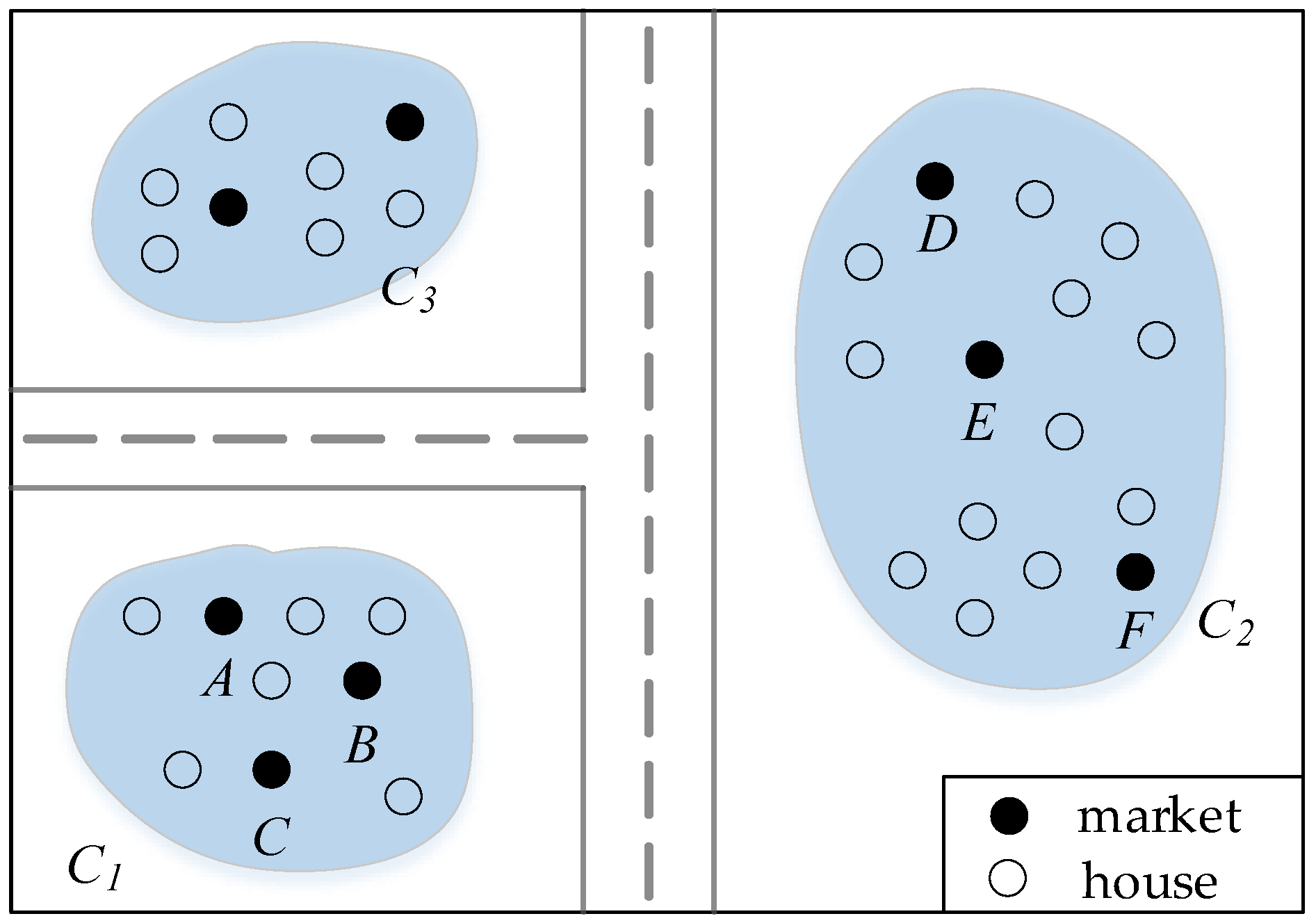
In Figure 1, Markets A, B, C are close, and Markets D, E, F are close by distance. Depending on the density of the market and house, dense markets form a cluster, e.g., C₁ and C₂, and the cluster can be assumed as one commercial district. We can get the confidence and the support of beer→diaper for each cluster.

Figure 1. An example of association rule mining considering purchase location.

The support of beer→diaper is 0.8 (4/5), and the confidence of beer→diaper is 1 (4/4) in C₁. The support of beer→diaper is 0.2 (1/5), and the confidence of beer→diaper is 0.25 (1/4). Even if the minimum support and confidence are set to 0.5, we can find the association rule with beer→diaper [sup: 0.8, conf: 1]. For example, data analysts can infer that there is a lot of households with babies around the C₁ commercial district from these association rules. With this knowledge, it is possible to set up a strategy for promoting baby products in the market of the relevant commercial district. In this way, association rules that were not discovered when analyzing the entire data can be discovered in data generated in a specific region. Association rules discovered in a specific region can be used as information to analyze the purchasing patterns or behavioral characteristics of consumers in that region. Until now, many association rule algorithms have been developed to discover association rules in the entire data, but no algorithm has yet been proposed to discover association rules effectively in partial transactions.

In this paper, we propose region-based FP-Growth (RFP-Growth) that discovers frequent patterns for each divided cluster after dividing the entire transaction data into density-based clusters. RFP-Growth algorithm generates FP-Tree with only transactions in those regions when the regions to find the association rule is selected. RFP-Growth discovers discover new frequent rules that were not found in the whole data. The contributions of this paper are summarized as follows.

• We proposed a novel problem of discovering association rules in item transactions considering the item purchase location.
• We proposed RFP-Growth which organizes item transaction data with location data into clusters by dense regions and discovers association rules for each cluster.
• We conducted extensive experiments on the real and synthetic datasets to prove that RFP-Growth discovers the new frequent rules that are not discovered in the analysis of the entire data.

The rest of this paper is organized as follows. Section 2 reviews related works to spatial clustering algorithms with FP-Growth and defines the problem. In Section 3, we describe an overview of RFP-Growth. In Section 4, we present experimental results and their evaluation. In Section 5, we conclude our work and present some directions for future research.

2. Background and Related Works

2.1. Background: FP-Growth

Apriori algorithm is the most representative algorithm for association rules and is a useful algorithm for finding frequent itemsets for binary association rules [9,17]. However, since candidate itemsets are repeatedly generated and the support is calculated while scanning the database, a lot of processing time is consumed. To compensate for this drawback, several studies have been conducted to reduce the number of candidate sets or the number of database scans. FP-Growth algorithm is attracting attention because it can analyze frequent patterns with only two database scans without generating a candidate set [10,18]. Important and quantitative information about frequent itemsets is stored in an extended prefix tree structure called FP-Tree. FP-Tree generates a frequency pattern tree with only two database scans. The priority of items is determined by counting the number of frequent occurrences of each item through the first database scan. Each set of items entered through the second database scan is sorted using the number of frequent occurrences.

A simple example of constructing FP-Tree is shown in Figure 2. Figure 2a is an example transaction database for creating FP-Tree (the minimum support is set to three). Each row is composed of a set of items that occur simultaneously within one transaction and is classified by transaction identification (TID). To construct FP-Tree using this example transactional database, first, we need to find the frequency of the items. The database is scanned once for the first time to count the number of items represented in the database. Then, in order to make a list of frequent items, only items with a minimum support rating or higher are used to create the FP-Tree in the order of the highest frequency. Figure 2b shows items with a frequency greater than or equal to the minimum support in the order of the highest frequency.

Figure 2. An example of transaction database and ordered and truncated transactional database.

The next step is to scan the transaction database a second time to construct FP-Tree. Starting from the root, transactions are added one by one to the root subtree in a prefix tree method. After reading each transaction, the items are reordered in reverse order of frequency. Items that do not meet the minimum support are not considered. Figure 2c shows the transaction after omitting items with a support rating of less than three from Figure 2a.

Figure 3 shows that the process of construction of FP-Tree. The process consisted of the four-step to add the five transactions of Figure 2a to FP-Tree. Figure 4 shows the final FP-Tree and its header table for the transaction database. FP-Tree reduces frequent database scans compared to Apriori algorithm. Since FP-Tree does not generate candidate sets, it is useful for finding frequent itemsets from large amounts of data. However, when the depth of the tree increases and the number of nodes increases, the dependence of the memory size is large, and a lot of processing time may be consumed for mining.

Figure 3. A process of FP-Tree construction. (a) Transaction (f,c,a,m,p) is inserted, (b) transaction (f,c,a,b,m) is inserted, (c) transaction (f,b) is inserted, (d) transaction (c,b,p) is inserted.

Figure 4. FP-Tree built based on the data in Figure 2a.

2.2. Variants of FP-Growth

Since the introduction of FP-Tree, various tree structures for frequency pattern mining such as COFI-tree [12], DRFP-tree [13,14], CanTree [15], DSTree [19], AFOPT-tree [20], CATS Tree [21], were presented. Since FP-Tree reads the entire database and constructs a tree using the number of frequent items, it is a data mining technique that applies only to a fixed database and cannot be used in a streaming database. In order to overcome the constraints of FP-Tree, DS-Tree for mining association rules in a streaming database is presented. DS-Tree does not use the number of frequent items but sorts the items according to the criteria set by the user so as to fit the characteristics of items such as alphabetical order or lexical order. After sorting, DS-tree is created by reading a batch, which is a set of transactions as much as the window size. DS-Tree is a tree construction method that can be applied not only to a fixed database but also to a data stream environment. While FP-Tree uses the number of item frequency as the item sorting criterion, DS-Tree uses a simple criterion such as alphabetical order or lexicographic order as a criterion for tree construction. Therefore, because the database scan to find the item sorting criteria can be omitted, a tree can be constructed with only one database scan, and a tree can be constructed even in a data stream environment. Since only one data scan is required, the time it takes to construct the tree can be reduced.

2.3. FP-Growth Based on Spatial Data

With the increase in spatiotemporal data, the problem of discovering spatiotemporal association rules in spatiotemporal databases has received considerable attention in the field of frequent pattern discovery. In addition, research on spatial frequent pattern analysis based on FP-Growth is being actively conducted.

Maiti et al. [22] proposed a Map-Reduce-based approach as a method of finding co-location patterns defined with R-proximity measure and conditional probability. The purpose of this approach is to find co-location patterns of all sizes from distributed data. The colocation rule is a model for inferring the existence or nonexistence of spatial features around the item by using the features of the item included in the rule. This approach consists of four algorithms, and FP-Growth algorithm is utilized as one method to find colocation by finding all frequent itemsets.

Lee et al. [23] proposed SFP-Growth algorithms to find spatial frequent patterns from social data. This study divides the entire space into cells on a 2D grid and manages cells hierarchically by dividing the side of a cell by four. The SFP-Growth algorithm extracts spatial frequent patterns of specific locations which explain the relative characteristics of the location. However, in this method, when a frequent pattern is extracted as the sum of distant lower cells included in the same upper cell, the frequent pattern becomes information describing the characteristics of the upper cell. In the upper cell, there are also lower cells that are not involved in the frequent pattern extraction at all. In this case, even cells that do not affect the frequent pattern extraction may be misinterpreted as having the frequent pattern property defined in the upper cell.

Kiran et al. [24] proposed frequent spatial pattern growth (FSP-Growth). This study defined interesting spatial patterns, including not only frequent items that occurred at close distances between two items but also items in which the maximum distance between two items was not greater than the user-specified maxDis.

2.4. Problem Definition

Let I = {i₁, i₂, …, i_n} be a set of n binary attributes called items. Let D = {t₁, t₂, …, t_m} be a set of transactions called the database. Let R = {r₁, r₂, …, r_k} be a set of k density regions. Each transaction in D has a unique transaction ID, a region where the product was purchased, and contains a subset of the items in I. A rule is defined as an implication of the form:

r: X→Y, where X, Y⊆I and r⊆R.

(1)

In order to select interesting rules from the set of all possible rules, constraints on various measures of significance and interest are used. The best-known constraints are minimum thresholds on support and confidence.

Let X, Y be itemsets and r be regions, r: X→Y an association rule, and T a set of transactions of a given database.

Definition 1.

(Support) Support is an indication of how frequently the itemset appears in the dataset. The support of X with respect to T is defined as the proportion of transactions t in the dataset which contains the itemset X.

supp(X, r) = |{t∈T; X⊆t}|/|T|, where T.region = r

The support gives an idea of how frequent an itemset is in all the transactions.

Definition 2.

(Confidence) Confidence is an indication of how often the rule has been found to be true. The confidence value of a rule, X→Y, with respect to a set of transactions T, is the proportion of the transactions that contain X which also contains Y.

conf(X→Y, r) = supp(X∪Y)/supp(X), where T.region = r

(2)

We modified by adding the locality of the transaction to the support and confidence used in the existing association rule. For conciseness of expression, however, it is expressed in the same way as support and confidence.

Problem definition. Given a set of transactions, D, containing regions where the items were purchased, the problem of mining association rules is to generate all association rules that have support and confidence greater than the user-specified minimum support (called minsup) and minimum confidence (called minconf) respectively for user-specified regions.

3. Methods

3.1. Overview of RFP-Growth

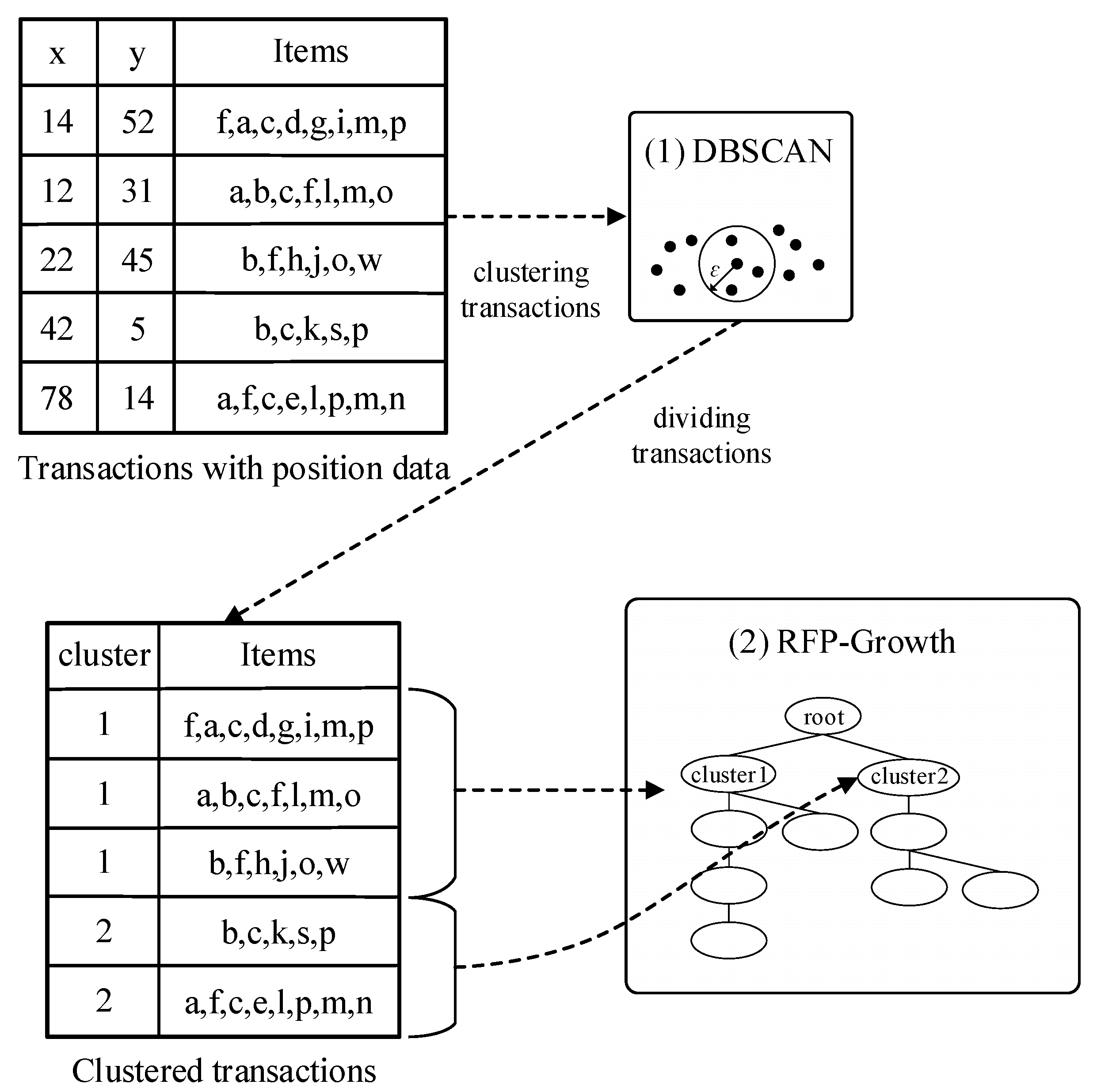
The purpose of this study is to prove that, if frequent rules are discovered by classifying transactions by region, frequent rules that cannot be discovered in the entire data can be found. RFP-Growth first divides transactions into density-based regions. The position data could be the name or code of the store where the transaction occurred, or it could be the longitude or latitude where the transaction occurred. We assume that the raw data to be analyzed contains longitude(x) and latitude(y) data where the transaction occurred.

DBSCAN performs the clustering process using only the location data of the raw data. Through the DBSCAN, each transaction is assigned to a cluster. In Figure 5, the cluster column means the cluster number to which each transaction is assigned in the clustered transaction table. For each cluster, RFP-Tree is generated using the transaction assigned to the cluster.

Figure 5. Overview of RFP-Growth.

3.2. Intersection-Based FP-Tree

The existing FP-Tree constructs a tree based on the criterion of the frequency of occurrence. However, in this paper, a method of constructing FP-Tree using the intersection is adopted. RFP-Tree based on the intersection is not a method of organizing a tree by sorting items using a specific criterion, but by grouping items generated by intersection each time each transaction is entered. Only one item may be included in one node, or multiple items may be included in one node. There is no need to rearrange the items in the transaction, and there is no need to build a new tree even if a continuous transaction flows in. When a new subtree is created, the item set with the highest frequency including the input transaction among the item sets is made as to the parent node. Therefore, the latest item frequency is continuously applied to the node can be optimized whenever a transaction is entered.

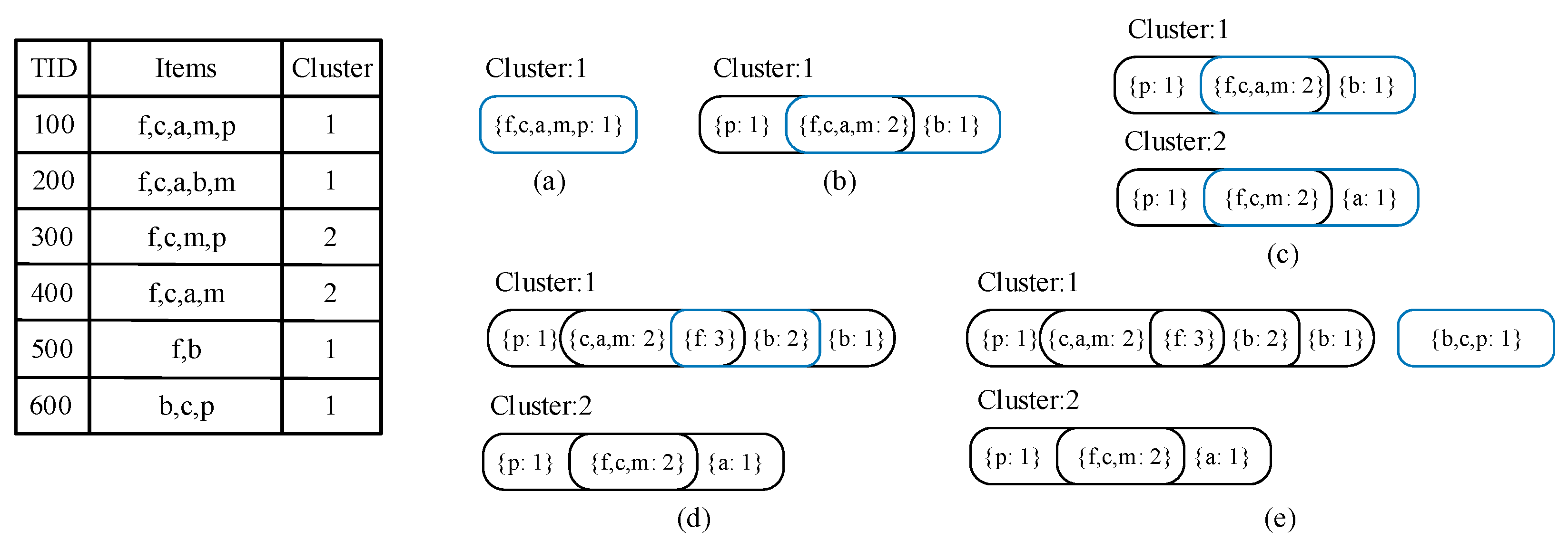
Figure 6 and Figure 7 show a process to construct RFP-Tree using the example of a transactional database in the aggregate expression method and tree structure. In the case of transactions 100 and 200 in Figure 6b, the intersection of two sets {f,c,a,m} was generated twice, and the {p} and {b} item sets were generated once. If this is presented as a tree, it can be expressed as shown in Figure 7b. Whenever a transaction is entered one by one, the item sets are finally grouped using the intersection set similar to Figure 7e. If there are no items intersected with an item of an existing transaction, such as Transaction 600 in Figure 6, a new node is created in a tree. These nodes are not considered in the process of deriving the association rule. In this way, a tree can be constructed each time a transaction is added one by one without the process of scanning the entire transaction once.

Figure 6. Construction of intersection-based FP-Tree (blue circles indicate newly added transactions). (a) Transaction (f,c,a,m,p) is inserted, (b) transaction (f,c,a,b,m) is inserted, (c) transactions (f,c,m,p) and (f,c,a,m) are inserted, (d) transaction (f,b) is inserted, (e) transaction (b,c,p) is inserted.

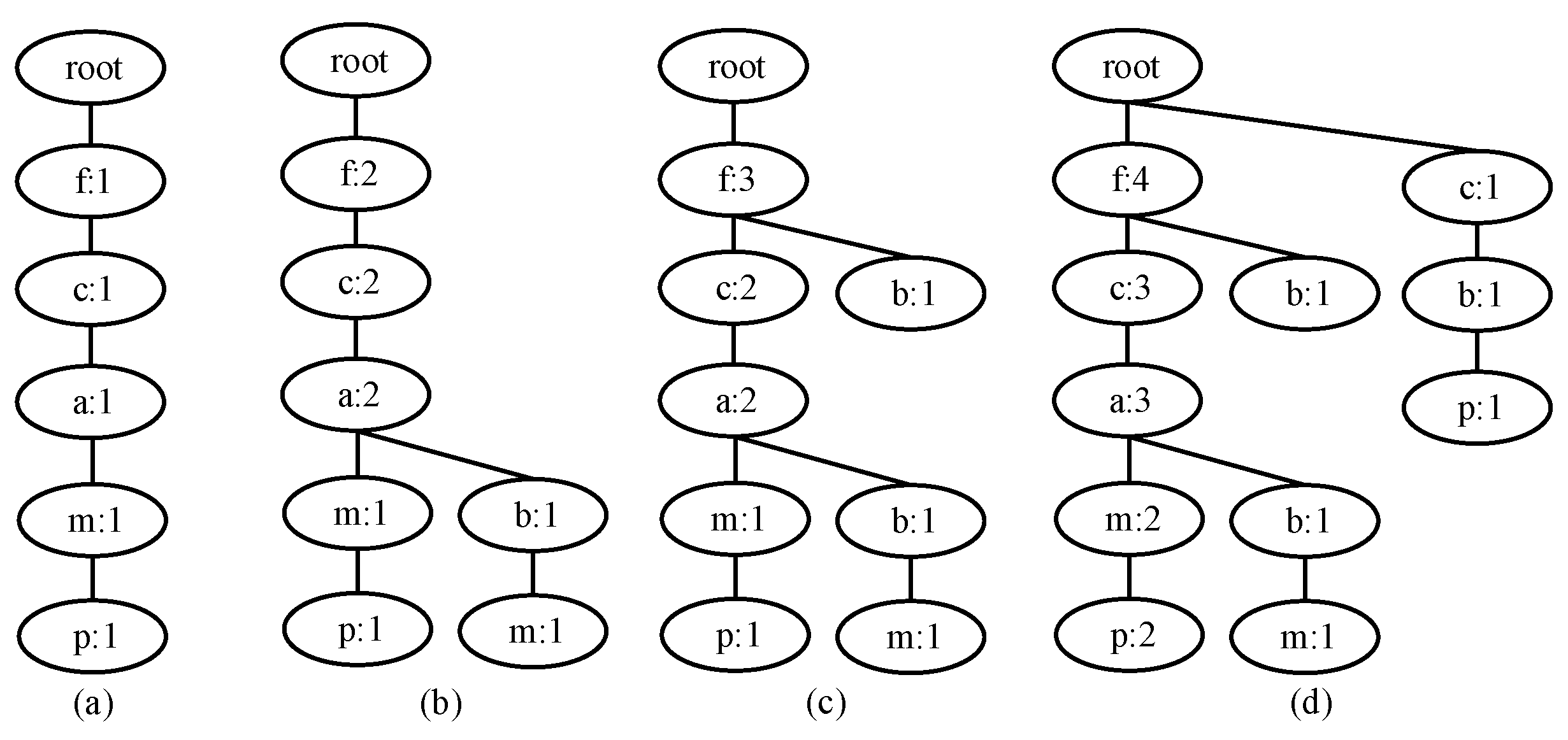
Figure 7. Tree representation of RFP-Tree. (a) Transaction (f,c,a,m,p) is inserted, (b) transaction (f,c,a,b,m) is inserted, (c) transactions (f,c,m,p) and (f,c,a,m) are inserted, (d) transaction (f,b) is inserted, (e) transaction (b,c,p) is inserted.

A general FP-Tree construction scans the entire database, which is the preprocessing step of tree construction, calculates the number of items, and uses this to rank the items, sort the items in each transaction in the reverse order of the number of items. However, since RFP-Tree does not require the pre-processing step of such tree configuration, it reads the database transaction and proceeds to construct the tree, thus reducing the pre-processing cost. A general FP-Tree composes a tree by reading one transaction from a database and reading items in the transaction one by one, but the proposed FP-Tree reads one transaction and constructs FP-tree in units of transactions, which reduces the cost of time compared to a general FP-Tree.

In general, the study of extracting association rules from spatial data first divides the data into clusters and then applies the traditional association rule mining algorithm to each cluster to find association rules. Instead of creating a tree after the DBSCAN process is finished, a tree can be constructed at the same time as one cluster is constructed in DBSCAN.

A transaction consists of <TID, region, items >where TID means a unique identifying number and region means a market where the consumer purchased the item and items mean the list of items purchased by consumers.

Algorithm 1 shows how RFP-tree is built. Through the entire transaction scan, only transactions with a given region from the user are selected in each transaction. For each transaction, the treeConstruct function is called and an item is passed as a parameter (Lines 2–4). If the intersection of the item of the child node (childNode) and the items of the current transaction is an empty set, items are inserted into the child of the current node (currentNode) (Lines 6–7). childNode means child node of currentNode. If the intersection of the item of the child node (childNode) and the items of the current transaction is not an empty set, a new node is added to the FP-Tree (Lines 8–23). If items and items of child node are the same, increase the frequency of child node by 1. If the items are a subset of the items of a childNode, insert the result of the difference between childNode and items in child of childNode. The intersection of childNode and items is reinserted in childNode. The frequency of childnode is increased by 1 (Lines 11–14). If the items of a childNode are a subset of the items, the frequency of the childNode is increased by 1. The result of the difference between items and items of childNode is inserted into restItems. treeConstruct function with restItem and childNode set as parameters is executed (Lines 15–18). If it is not included in the above three cases, two child nodes are created (Lines 20–21). The difference between childNode and items is inserted into the first child node (Line 20), and the difference between items and childNode is inserted into the second child node (Line 21). The intersection of childNode and items is reinserted in childNode and the frequency of childNode is increased by 1 (Lines 20–23).

Algorithm1 TreeBuilder

Input: A transaction DB, a set Q of query keywords, a set R of region Output: FP-tree 1. NODE node = null; 2. for each transaction t∈DB do 3.       if t.region ∊ R then 4.            treeConstruct(t.items, node) 5. Procedure treeConstruct(items, currentNode) 6.           if childNode.items ∩ items == $\varnothing$ then 7.                currentNode.child ← items 8.           else 9.                if childNode.items == items then 10.                   childNode.frequency++ 11.              else if childNode.items ⊃ items then 12.                   childNode.child ← childNode–items 13.                   childNode = childNode ∩ items 14.                   childNode.frequency++ 15.              else if childNode.items ⊂ items then 16.                       childNode.frequency++ 17.                       restItems = items–childNode.items 18.                       treeConstruct(restItems, childNode); 19.                else // split and add node 20.                       childNode.child← childNode–items 21.                     childNode.child←items–childNode 22.                     childNode = childNode ∩ items 23.                     childNode.frequency++

Complexity. Existing FP-Tree construction algorithms require two database scans that need 2n, where n is the number of transactions. However, the RFP-Tree construction algorithm can create a tree with one database scan. Our proposed algorithms can reduce the number of transactions to n. Whenever a transaction is added one by one, the item comparison operation of the two transactions executes. The complexity of RFP-Tree construction algorithm is dominated by comparing two sets of elements. If the average number of items in one transaction is m, the number of times to compare common items in two transactions is m². Thus, the complexity of RFP-Tree construction algorithm is O(nm²).

4. Results and Discussion

4.1. Experiment Setting

4.1.1. Algorithms

The purpose of this study is to verify whether new association rules are found when the association rule is extracted by dividing a transaction database by region compared to when the association rule is extracted for the entire data. We compared RFP-Growth algorithm with the original FP-Growth, dFIN [25] and negFIN [26]. The FP-Growth algorithm discovers frequent patterns from the transaction that consists solely of items, while RFP-Growth algorithm considers the transaction with spatial data. RFP-Growth algorithm consists of two steps.

(1) The transaction is divided into regions by clustering on spatial data included in a transaction. We used DBSCAN algorithm, a clustering algorithm that allows clusters to have an arbitrary shape because we considered a commercial area with dense stores as one region. (2) FP-Growth algorithm is performed for each transaction divided by region.

All the proposed algorithms were implemented in Java, and the experiments were conducted on an Intel Core i7 at 3.50 GHz with 32 GB memory. The parameters used for the experiments are summarized and default values are shown in boldface in Table 2.

Table 2. Parameters for the experiments.

Parameters	Description	Values
n	no. of objects	1K, 2K, 3K, 4K, 5K, 6K, 7K, 8K, 9K, 10K
k	no. of clusters	5, 10, 15, 20, 25
minsup	minimum support	0.20, 0.22, 0.24, 0.26, 0.28, 0.30, 0,32, 0,34, 0.36, 0.38, 0.40, 0.42, 0.44, 0.46, 0.48, 0.50, 0.52, 0.54, 0.56, 0.58, 0.60, 0.62, 0.64, 0.66, 0.68, 0.70

“K” represents 1000.

4.1.2. Data Sets

The real-world datasets and synthetic data sets are used for experiments. For a real dataset, we collected sets of purchase items made for an online retail company based in the UK during an eight-month period (https://www.kaggle.com/vijayuv/onlineretail (accessed on 1 December 2021)). The real dataset consists of 25,900 transactions, and there are 4070 items. Table 3 shows samples of real datasets. We removed unnecessary columns for the experiment, i.e., Quantity, Invoice Date, Unit Price, and Customer ID. Since the same transaction is divided into several rows, the rows of the same invoice number are combined into one row. We conducted an experiment assuming the same country as one cluster by using the country column as location information. For the synthetic data, spatial data are generated in the 2D space (0, 100) × (0, 100) to indicate a store’s location, and item data are generated among 100 items totally. Items in the synthetic data are generated so that there are no duplicate items in one transaction which has an average of 20 items.

Table 3. Samples of a real dataset.

Invoice No.	Stock Code	Quantity	Invoice Date	Unit Price	Customer ID	Country
536365	85123A	6	01-12-2010 08:26	2.55	17850	UK
536365	71053	6	01-12-2010 08:26	3.39	17850	UK
356365	84406B	8	01-12-2010 08:26	2.75	17850	UK
536370	22728	24	01-12-2010 08:45	3.75	12583	France
536370	22727	24	01-12-2010 08:45	3.75	12583	France
536370	22726	12	01-12-2010 08:45	3.75	12583	France
536389	22941	6	01-12-2010 10:03	8.5	12431	Australia
536389	22941	8	01-12-2010 10:03	4.95	12431	Australia
536389	22941	12	01-12-2010 10:03	1.25	12431	Australia

4.2. The Discovery of New Association Rules

In this section, we evaluate the effect with respect to the minsup on the discovery of new association rules. The Support means an indication of how frequently the itemset appears in the dataset. minsup is the minimum support for an itemset to be identified as frequent. The smaller the minsup, the more frequent rules are discovered. If the support of an itemset is low, there is not enough information about the relationships between items. We need to find support that elicits a reasonable number of frequent rules. We conduct experiments with various minsup [0.2, 0.7], and set n = 10,000 and k = 5. Since FP-Growth, dFIN, and negFIN algorithms yield the same rules as a result, we compared the results of the FP-Growth algorithm to see if RFP-Growth algorithm discovers new rules.

Figure 8 shows the number of newly discovered frequent rules according to the support level from the synthetic datasets. The left y-coordinate represents the number of the frequent rules found in FP-Growth. The right y-coordinate represents the number of the frequent rules that are not found in FP-Growth and are newly discovered in RFP-Growth. As minsup becomes larger, the number of the frequent rules discovered decreases. As minsup increases, the number of newly discovered rules decreases. In the section where the number of the frequent rules discovered in FP-Growth is maintained, [0.22–0.3, 0.34–0.44, 0.5–0.68], the number of newly discovered frequent rules in RFP-Growth is low. It can be seen that when the number of the frequent rules discovered in FP-Growth is reduced, the number of the frequent rules newly discovered in RFP-Growth increases. When minsup was 0.7, no rules were discovered in FP-Growth, but 20 rules were discovered in RFP-Growth.

Figure 8. The number of discovered frequent rules in FP-Growth and RFP-Growth from the synthetic data.

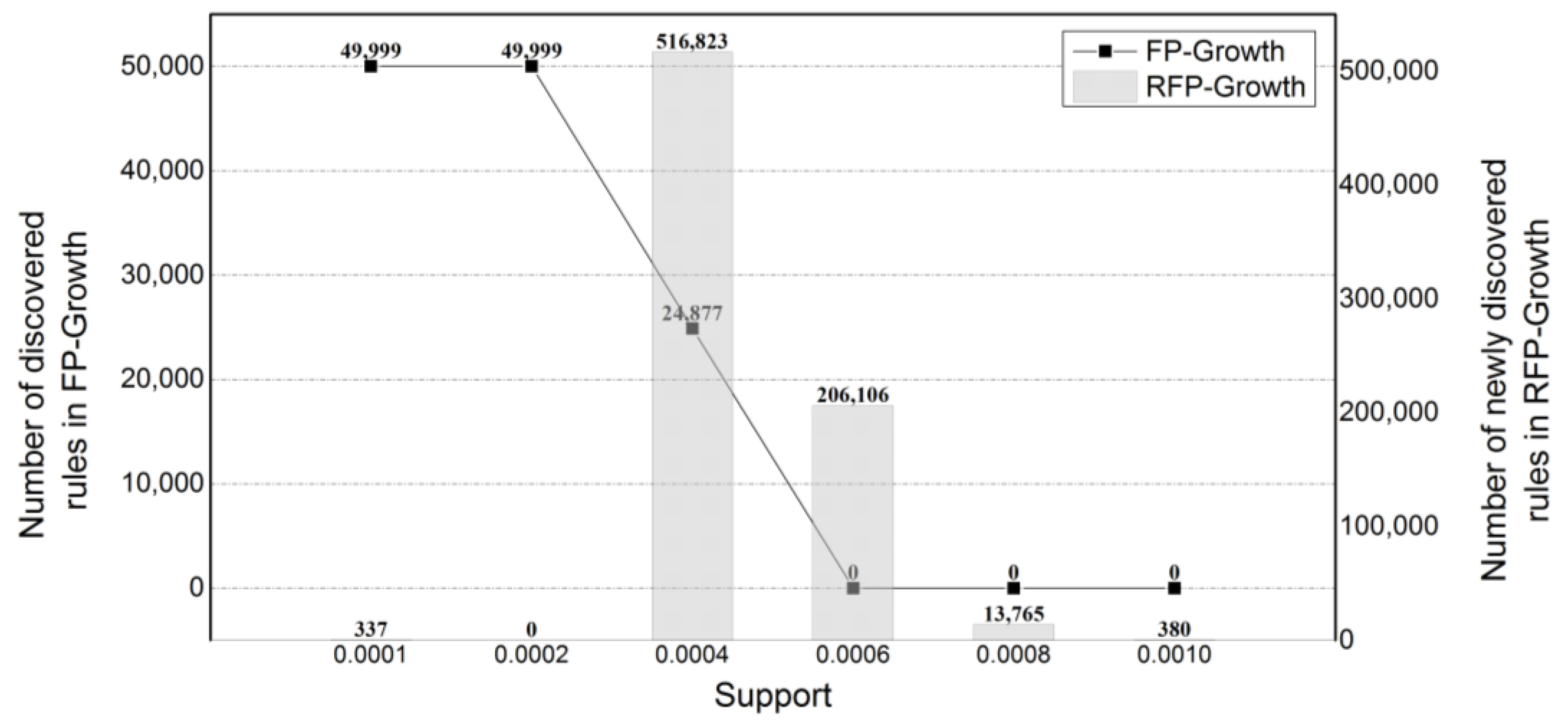
Figure 9 shows the number of newly discovered frequent rules according to the support level from the real datasets. The left y-coordinate represents the number of the frequent rules found in FP-Growth. The right y-coordinate represents the number of the frequent rules that are not found in FP-Growth and are newly discovered in RFP-Growth. We conduct experiments with various minsup [0.0001, 0.001], and set n = 1,044,000 and k = 50. In the section where the number of the frequent rules discovered in FP-Growth is maintained, [0.0001–0.0002, 0.0006–0.001], the number of newly discovered frequent rules in RFP-Growth is low. It can be also seen that when the number of the frequent rules discovered in FP-Growth is reduced, the number of the frequent rules newly discovered in RFP-Growth increases. When minsup was 0.0006, 0.0008 and 0.001, no rules were discovered in FP-Growth, but 206,106, 13,765 and 380 rules were discovered in RFP-Growth respectively.

Figure 9. The number of discovered frequent rules in FP-Growth and RFP-Growth from the real-world data.

4.3. Memory Consumption

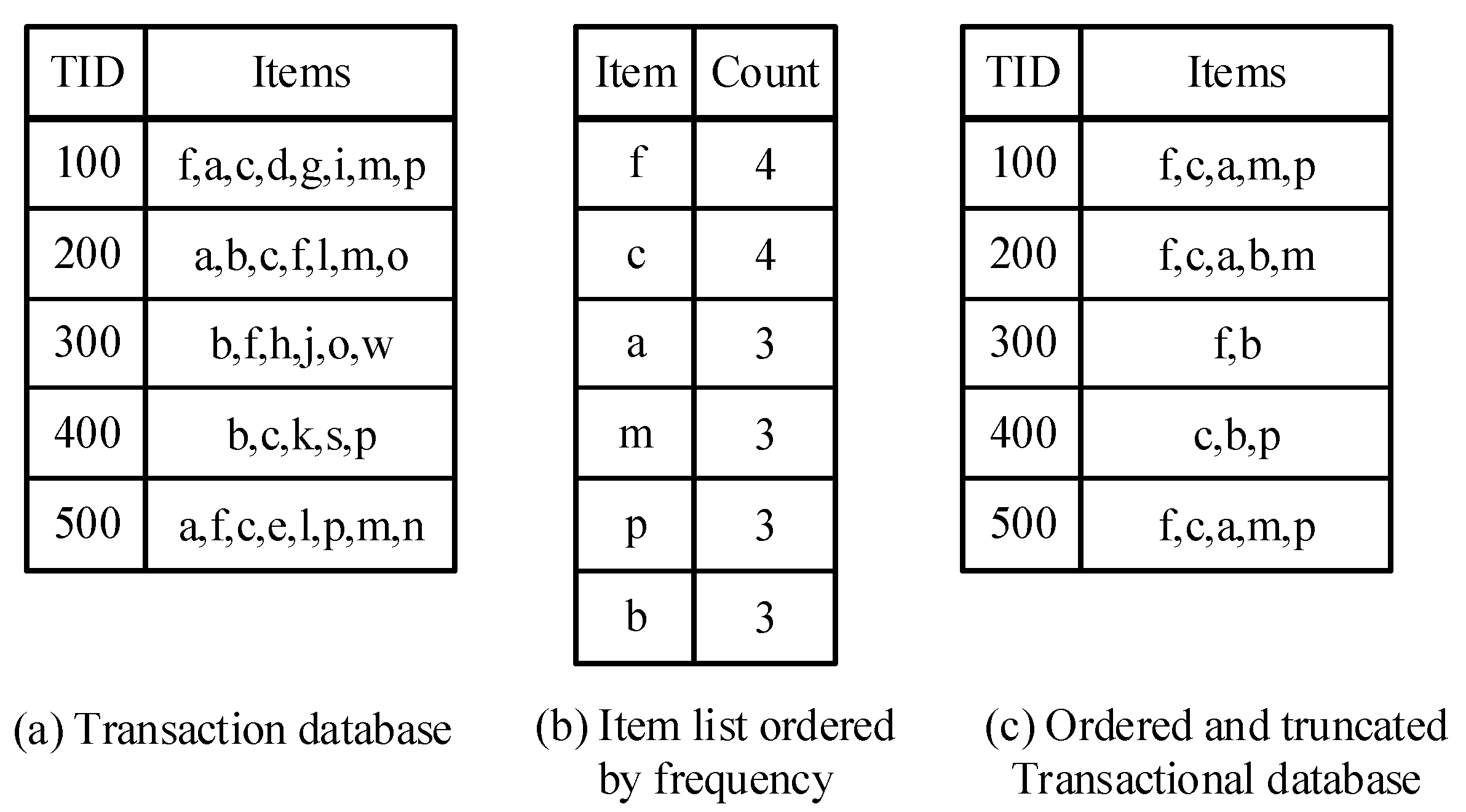
In this section, we measure the memory consumption with respect to the minsup for the real-world datasets and the synthetic datasets. Figure 10 shows that the larger the minsup, the smaller the memory usage. This is because, in general, as minsup increases, the number of items treated as a frequent pattern decreases. Comparing the memory usage of RFP-Growth and FP-Growth, it was found that the memory usage decreased by 34% for synthetic datasets and 23% for real datasets. This can be explained as follows. RFP-Growth generates an FP-Tree from transaction data through an intersection operation, whereas FP-Growth generates an FP-Tree after creating an ordered and truncated transactional table in Figure 2c. dFIN and negFIN show higher memory usage than FP-Growth for low minsup.

Figure 10. Memory consumption comparison for different datasets, depending on the minsup. (a) Synthetic datasets, (b) real-world datasets.

The runtime comparison of RFP-Growth against FP-Growth, dFIN, and negFIN with respect to the minsup is shown in Figure 11. In all algorithms, it appears that the runtime cost decreases as minsup increases. The best performance at runtime is negFIN, which is known as the fastest algorithm, followed by dFIN, RFP-Growth, and FP-Growth. RFP-Growth shows better performance than FP-Growth, and the runtime performance of RFP-Growth is slightly lower than dFIN and negFIN. Although RFP-Growth uses less memory, it seems that the set operation to find common items increases the time cost.

Figure 11. Run time cost comparison for different datasets, depending on the minimum support. (a) Synthetic datasets, (b) real-world datasets.

4.4. The Effect of the Number of Clusters

In this section, we evaluate the effect with respect to the number of clusters for the real-world datasets and the synthetic datasets. We conduct experiments with the various clusters [5, 10, 15, 20, and 25]. In the synthetic datasets, we set n = 10,000, minsup = [0.32, 0.48] and k = 5. In the real-world datasets, we set n = 1,044,000, minsup = [0.0006, 0.0008] and k = 50.

Figure 12 shows the effects of the number of clusters on the number of newly discovered frequent rules in RFP-Growth. Two graphs are also shown on a linear scale. For each dataset, the number of newly discovered frequent rules in RFP-Growth is approximately proportional to the number of clusters. In both graphs, when minsup is high (0.48, 0.006), the number of newly discovered frequent rules gradually increases. On the other hand, when minsup is low (0.32, 0.008), the number of newly discovered rules increases rapidly as the number of clusters increases.

Figure 12. The number of discovered frequent rules with respect to the number of clusters in RFP-Growth. (a) Synthetic datasets, (b) real-world datasets.

Figure 13 shows the effects of the number of clusters on the time cost in RFP-Growth. Two graphs are also shown on a linear scale. For each dataset, the time cost in RFP-Growth is approximately proportional to the number of clusters. In the synthetic datasets, the time cost is different for the two minsup (0.32 and 0.48), but in the real dataset, there is little difference in the time cost for the two minsup (0.0006 and 0.0008). This difference is caused by the difference in scale for the two datasets. What we can see from this result is that the time cost increases as the number of clusters increases.

Figure 13. Time cost with respect to the number of clusters in RFP-Growth algorithm. (a) Synthetic datasets, (b) real-world datasets.

4.5. The Effect of the Size of Data

To illustrate scalability, we vary the number of objects from 1K to 10K for the synthetic datasets. Other parameters are given their baseline values (Table 2). Figure 14 shows the effect of the number of objects in FP-Growth, dFIN, negFIN, and RFP-Growth. This graph is shown on a linear scale. For each algorithm, the runtime is approximately proportional to the number of objects. As shown in Figure 14, the time cost of RFP-Growth algorithm is lower than the time cost of FP-Growth. It can be seen that processing the divided data after dividing the data into several groups is faster than processing the entire data at once.

Figure 14. Effect of the size of datasets.

5. Conclusions

In this paper, we proposed the noble problem of discovering association rules by regions. Toward this goal, we proposed RFP-Growth, which organizes item transaction data with location data into groups and discovers association rules for each cluster. RFP-Growth divides item transaction included position data into regions by a density-based clustering algorithm. FP-Growth is performed for each transaction divided by region. The experimental results show that RFP-Growth discovers new association rules that the original FP-Growth cannot find in the whole data. RFP-Growth has a disadvantage, however, that the performance decreases as the number of clusters increases. In future work, we plan to improve the performance of RFP-Growth, so even if the number of clusters increases, the performance is stabilized.

References

1. Alshammari, H.; El-Ghany, S.A.; Shehab, A. Big IoT Healthcare Data Analytics Framework Based on Fog and Cloud Computing. J. Inf. Process. Syst. 2020, 16, 1238–1249. [Google Scholar]
2. Qi, J.; Yang, P.; Hanneghan, M.; Tang, S.; Zhou, B. A Hybrid Hierarchical Framework for Gym Physical Activity Recognition and Measurement Using Wearable Sensors. IEEE Internet Things J. 2019, 6, 1384–1393. [Google Scholar] [CrossRef]
3. Wang, T.; Qiu, L.; Sangaiah, A.K.; Liu, A.; Alam Bhuiyan, Z.; Ma, Y. Edge-Computing-Based Trustworthy Data Collection Model in the Internet of Things. IEEE Internet Things J. 2020, 7, 4218–4227. [Google Scholar] [CrossRef]
4. Al-Shargabi, A.; Siewe, F. A Lightweight Association Rules Based Prediction Algorithm (LWRCCAR) for Context-Aware Systems in IoT Ubiquitous, Fog, and Edge Computing Environment. In Proceedings of the Proceedings of the Future Technologies Conference (FTC) 2020, Vancouver, BC, Canada, 5–6 November 2020. [Google Scholar] [CrossRef]
5. Lee, C.H.; Park, J.S. An SDN-Based Packet Scheduling Scheme for Transmitting Emergency Data in Mobile Edge Computing Environments. Hum. Cent. Comput. Inf. Sci. 2021, 11. [Google Scholar] [CrossRef]
6. He, Y.; Tang, Z. Strategy for Task Offloading of Multi-user and Multi-server Based on Cost Optimization in Mobile Edge Computing Environment. J. Inf. Process. Syst. 2021, 17, 615–629. [Google Scholar]
7. Lee, J.-H. Next Task Size Prediction Method for FP-Growth Algorithm. Hum. Cent. Comput. Inf. Sci. 2021, 11. [Google Scholar] [CrossRef]
8. Agrawal, R.; Imieliski, T.; Swami, A. Mining association rules between sets of items in large databases. In Proceedings of the ACM SIGMOD Record, New York, NY, USA, 1 June 1993; Volume 22, pp. 207–216. [Google Scholar]
9. Agrawal, R.; Srikant, R. Fast algorithms for mining association rules in large databases. In Proceedings of the 20th International Conference on Very Large Data Bases, San Francisco, CA, USA, 12–15 September 1994; pp. 487–499. [Google Scholar]
10. Han, J.; Pei, J.; Yin, Y. Mining Frequent Patterns without Candidate Generation. ACM SIGMOD Rec. 2000, 29, 1–12. [Google Scholar] [CrossRef]
11. Giannella, C.; Han, J.; Pei, J.; Yan, X.; Yu, P.S. Mining Frequent Patterns in Data Streams at Multiple Time Granularities. In Data Mining: Next Generation Challenges and Future Directions; Kargupta, H., Joshi, A., Sivakumar, K., Yesha, Y., Eds.; AAAI Press: Palo Alto, CA, USA, 2004. [Google Scholar]
12. Zaïane, O.R.; El-Hajj, M. COFI Approach for Mining Frequent Itemsets Revisited. In Proceedings of the 9th ACM SIGMOD Workshop on Research Issues in Data Mining and Knowledge Discovery, Paris, France, 13 June 2004; pp. 70–75. [Google Scholar]
13. Adnan, M.; Alhajj, R. DRFP-tree: Disc-resident frequent pattern tree. Appl. Intell. 2009, 30, 84–97. [Google Scholar] [CrossRef]
14. Adnan, M.; Alhajj, R. A bounded and Adaptive Memory-based Approach to Mine Frequent Patterns from Very Large Databases. IEEE Trans. Syst. Man Cybern. Part B 2011, 41, 154–172. [Google Scholar] [CrossRef] [PubMed]
15. Leung, C.K.-S.; Khan, Q.I.; Hoque, T. CanTree:A Tree Structure for Efficient Incremental Mining of Frequent Patterns. In Proceedings of the Fifth IEEE International Conference on Data Mining (ICDM’05), Houston, TX, USA, 27–30 November 2005; pp. 274–281. [Google Scholar]
16. Ünvan, Y.A. Market basket analysis with association rules. Commun. Stat. Theory Methods 2021, 50, 1615–1628. [Google Scholar] [CrossRef]
17. Mar, Z.; Oo, K.K. An Improvement of Apriori Mining Algorithm using Linked List Based Hash Table. In Proceedings of the 2020 International Conference on Advanced Information Technologies (ICAIT), Yangon, Myanmar, 4–5 November 2020. [Google Scholar] [CrossRef]
18. Pan, Z.; Liu, P.; Yi, J. An Improved FP-Tree Algorithm for Mining Maximal Frequent Patterns. In Proceedings of the 2018 10th International Conference on Measuring Technology and Mechatronics Automation (ICMTMA), Changsha, China, 10–11 February 2018. [Google Scholar] [CrossRef]
19. Leung, C.K.-S.; Khan, Q.I. DSTree: A tree structure for the mining of frequent sets from data streams. In Proceedings of the Sixth International Conference on Data Mining (ICDM’06), Hong Kong, China, 18–22 December 2006; pp. 928–932. [Google Scholar]
20. Liu, G.; Lu, H.; Yu, J.X.; Wang, W.; Xiao, X. AFOPT: An efficient implementation of pattern growth approach. In Proceedings of the ICDM Workshop, Melbourne, FL, USA, 19–22 November 2003. [Google Scholar]
21. Cheung, W.; Zaiane, O.R. Incremental mining of frequent patterns without candidate generation or support constraint. Database Engineering and Applications Symposium. In Proceedings of the Seventh International Database Engineering and Applications Symposium, Hong Kong, China, 18 July 2003; pp. 111–116. [Google Scholar]
22. Maiti, S.; Subramanyam, R.B.V. Mining co-location patterns from distributed spatial data. J. King Saud Univ. Comput. Inf. Sci. 2020, 33, 1064–1073. [Google Scholar] [CrossRef]
23. Lee, Y.; Nam, K.W.; Ryu, K.H. Fast mining of spatial frequent wordset from social database. Spat. Inf. Res. 2017, 25, 271–280. [Google Scholar] [CrossRef][Green Version]
24. Kiran, R.U.; Shrivastava, S.; Fournier-Viger, P.; Zettsu, K.; Toyoda, M.; Kitsuregawa, M. Discovering Frequent Spatial Patterns in Very Large Spatiotemporal Databases. In Proceedings of the SIGSPATIAL ’20: 28th International Conference on Advances in Geographic Information Systems, Seattle, WA, USA, 3–6 November 2020; pp. 445–448. [Google Scholar] [CrossRef]
25. Deng, Z.-H. DiffNodesets: An Efficient Structure for Fast Mining Frequent Itemsets. Appl. Soft Comput. 2016, 41, 214–223. [Google Scholar] [CrossRef]
26. Aryabarzan, N.; Minaei-Bidgoli, B.; Teshnehlab, M. negFIN: An efficient algorithm for fast mining frequent itemsets. Expert Syst. Appl. 2018, 105, 129–143. [Google Scholar] [CrossRef]
Publisher’s Note: MDPI stays neutral with regard to jurisdictional claims in published maps and institutional affiliations.
Article Metrics
Citations
Article Access Statistics
Multiple requests from the same IP address are counted as one view.