Phase Role in the Non-Uniformity of Main-Line Couplings in Asymmetric Extracted-Pole Inline Filters

Abstract

The use of classical symmetrical polynomial definition to synthesize fully canonical inline filters with an asymmetrical distribution of the transmission zeros along the topology leads to the occurrence of uneven admittance inverter in the main-line. This form introduces some limitations to transform such topology into a ladder network. Despite circuital transformation can be used to accommodate both technology and topology, it is usual that extra reactive elements are necessary to implement phase shifts required to achieve the complete synthesis. This article introduces a novel method able to determine the required phase correction that has to be applied to the characteristic polynomials in order to equalize all the admittance inverters in the main path to the same value. It has been demonstrated that a suitable pair of phase values can be accurately estimated using a developed hyperbolic model which can be obtained from the transmission and reflection scattering parameters. To experimentally validate the proposed method, a Ladder-type filter with asymmetrical polynomial definition has been synthesized, fabricated, and measured, demonstrating the effectiveness of the developed solution.

1. Introduction

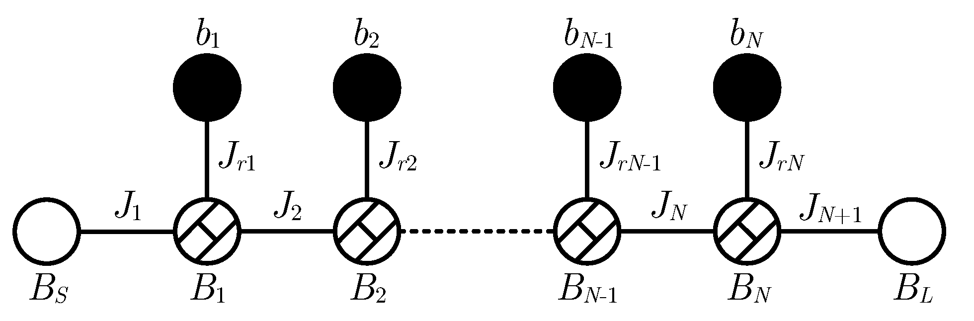
A general fully canonical lowpass prototype network consists of an array of N shunt-connected capacitors which are synthesized using a circuit elements extraction method. Fully canonical networks can be also successfully described with an inline filter topology allowing the use of the extracted pole synthesis technique [1,2,3,4]. The equivalent lowpass model configuration can be made of a series of dangling resonators between admittance inverters which are constituted by a combination of resonators nodes (RN) and non-resonator nodes (NRN) coupled to each other by means of immittance inverters $J_{rk}$ as depicted in Figure 1.

Usually, the dangling resonators are tuned to the transmission zero (TZ) and the non-resonant node prepares the extraction of the next finite TZ of $(i+1)$th dangling resonator. It is interesting to notice that it is not possible to determine both the main-line and the resonator admittance inverter, respectively, $J_k$ and $J_{rk}$, but only their ratio [5]. This useful property can lead to multiple solutions suitable for different types of technologies, providing the same transmission and reflection responses.

In the particular case of ladder topologies, the admittance inverters in the main-line $J_k$ do not exist physically because they are employed in pairs as an instrument to serialize shunt connected resonators [6]. There is a degree of freedom in setting their values, usually to unity for the sake of simplicity; however, alternation in sign along the source-to-load path is a necessary condition for further lowpass-to-bandpass elements transformation [7].

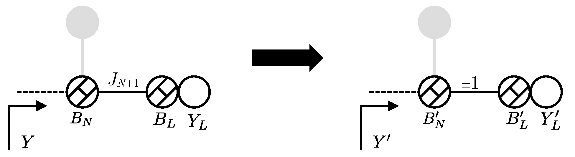
Depending on the filter specifications, it may occur that one $J_k$ cannot be scaled to the common value [1]. In this situation, the uneven admittance inverter can be moved close to the output port ($J_{N+1}$ in Figure 1), and apply an admittance redistribution in the last three elements of the network $B_N$, $J_{N+1}$ and $B_L$ with $|J_{N+1}|=$1. This redistribution process achieves the unitary inverter at the cost of modifying the output phase of the network.

Despite its simplicity and utility, the redistribution solution may not be convenient for every network. For some filter specifications, the admittance redistribution may require changing the impedance of the output port leading to an impedance mismatch. Moreover, in other cases it is not applicable, such as in cross-coupled topologies [8,9,10], where there are ladder networks with a source-to-load coupling embracing the whole main-line inverters. In such scenario, it is not possible to scale the network without changing the value of the coupling, which is not a feasible option.

To overcome this limitation, we propose a method based on the phase correction of the characteristic polynomials of the filtering function $F_{11}\left(s\right)$, $F_{22}\left(s\right)$ and $E\left(s\right)$. The phase modification method attains the same result as the admittance redistribution but modifying the phases of the input and output ports simultaneously in other to equalize all the admittance inverters in a fully canonical lowpass prototype. Unlike the admittance redistribution, a unity terminating output admittance $G_L$ is always achieved. In addition, the differentiated phase correction of $F_{11}\left(s\right)$, $F_{22}\left(s\right)$ may also be useful for duplexer design where one of the most important features is the isolation between transmitter and receiver filters. In [6,7], it is described that the loading effects in both filters can be minimized by modifying the input phase of each filter at the antenna port to a certain specific value. Therefore, by a proper phase correction, both conditions, homogeneous main-line admittance inverters and the phase match for duplexers can be achieved simultaneously.

The methodology to determine the required input/output phases strongly depends on the distribution of TZs as shown in [11] for odd-order filters. This paper extends the methodology for any class of filter, including also even-order filters, employing a precise mathematical model.

After describing the consequences of the uneven admittance inverter in fully canonical networks in Section 2, the current solutions and their limitations are discussed. To overcome this problem, the generation of asymmetrical polynomials is proposed in Section 3. In Section 4, the space map for suitable additional phase terms to be applied to the characteristics polynomials is explored for each case. The mathematical models and the systematic method to implement the proposed solution is thoroughly described in Section 5 for odd and even order filters. In Section 6, an independent experimental validation is reported. Finally, the conclusions are presented.

2. Uneven Admittance Inverters in Inline Fully Canonical Filters with Dangling Resonators

Generically, when the nodes in the main-line of the network are surrounded by admittance inverters, it is possible to scale the impedance at each node to arbitrary values, once the characteristic immittance of the inverters are set to the desired value. Basically, this is equivalent to adjust the transformer ratios of the input and output coupling transformers such that the total energy transferring through the node remains the same [12].

In ladder topologies, such as the one in Figure 1, homogeneous values in all main-line admittance inverters are required to succeed in the lowpass-to-bandpass elements transformation [7]. At each extraction iteration, the ratio of $J_k$ and $J_{rk}$ is obtained so $J_k$ can be set to $\pm 1$. However, the value for the last inverter $J_{N+1}$ is given by the remaining admittance to be extracted, so it cannot be set freely and its value will depend on the filter specifications, specifically, on the TZs distribution. When the TZs are allocated symmetrically with respect to the central resonator along the ladder topology, e.g., ${\Omega }_{Ak}=\{{\Omega }_1,{\Omega }_2,{\Omega }_3,{\Omega }_2,{\Omega }_1\}$, all the main-line admittance inverters, including $J_{N+1}$, can be scaled to $\pm 1$ successfully during the extraction procedure. However, if another type of TZs distribution is used, hereafter asymmetrical TZs distribution, such as ${\Omega }_{Bk}=\{{\Omega }_1,{\Omega }_2,{\Omega }_1,{\Omega }_2,{\Omega }_3\}$, an uneven admittance inverter in the main-line path with a different value than the rest will be required.

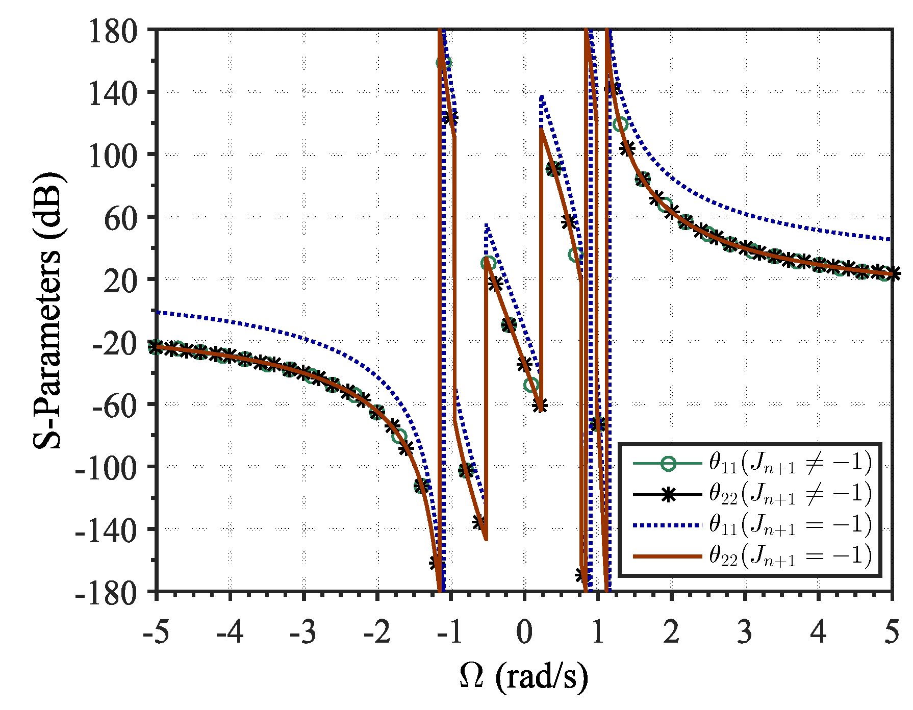
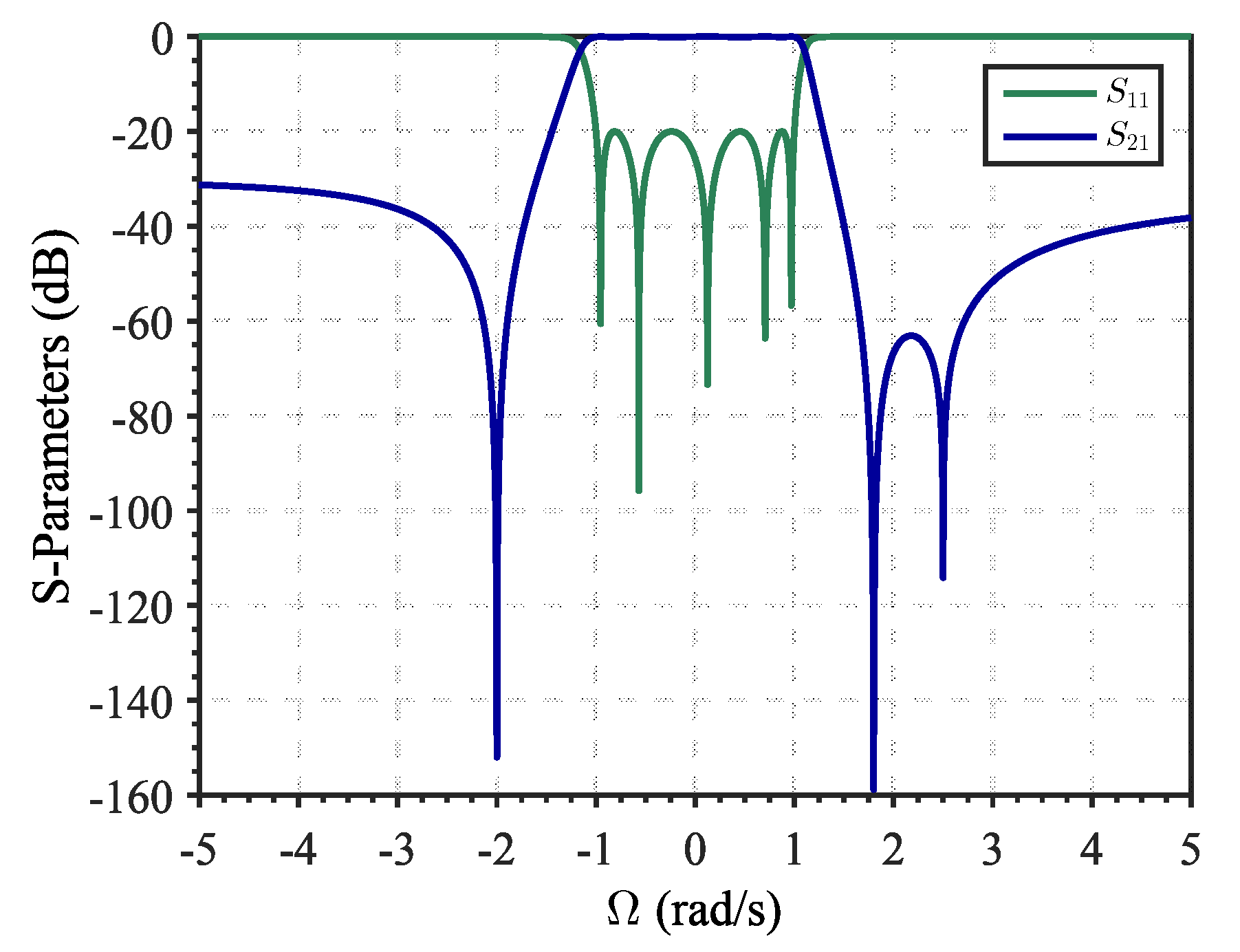
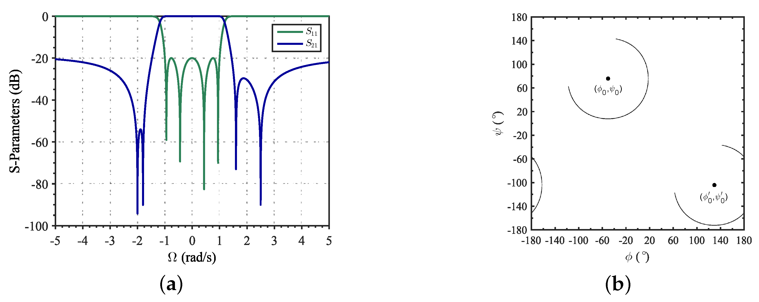
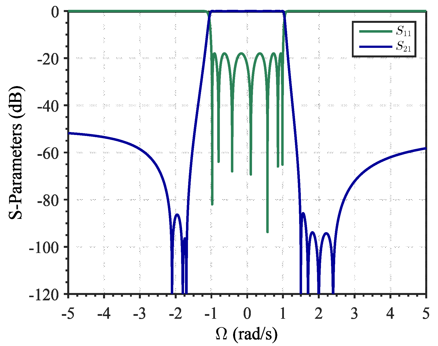
For instance, let us consider a filter with TZs at ${\Omega }_{Ak}=\{1.8,-2,2.5,-2,1.8\}$ rad/s and RL $=20$ dB. The resulting network scheme is similar to the one depicted in Figure 1, being the extracted filter elements listed in

Table 1. Extracted elements of the 5th-order filter prototype with ${\Omega }_{Ak}$ and ${\Omega }_{Bk}$ TZs distributions.

	${\mathbf{\Omega }}_{\mathit{Ak}}$			${\mathbf{\Omega }}_{\mathit{Bk}}$
Parameters	${\mathit{B}}_{\mathit{k}}$	${\mathit{b}}_{\mathit{k}}$	${\mathit{J}}_{\mathit{rk}}$	${\mathit{B}}_{\mathit{k}}$	${\mathit{b}}_{\mathit{k}}$	${\mathit{J}}_{\mathit{rk}}$
Res. 1	−1.0927	−1.8	1.1768	−1.0927	−1.8	1.1768
Res. 2	3.4897	2.0	2.4193	3.3440	2.0	2.4193
Res. 3	−2.6930	−2.5	2.6548	−1.8121	−1.8	1.7911
Res. 4	3.4897	2.0	2.4193	3.5215	2.0	2.4946
Res. 5	−1.0927	−1.8	1.1768	−1.4090	−2.5	1.7951
Source	−0.7388			−0.7388
Load	−0.7388			−0.4553

. In this case, the admittance inverters are $J_k=\{1,-1,1,-1,1,-1\}$. Since the TZs are symmetrically distributed at each side of ${\Omega }_{A3}=2.5$, their values are all unitary with alternated sign. However, with an asymmetrical TZs distribution such as ${\Omega }_{Bk}=\{1.8,-2,1.8,-2,2.5\}$ rad/s, in which ${\Omega }_{A3}$ and ${\Omega }_{A5}$ have been interchanged, the admittance inverters are $J_k=\{1,-1,1,-1,1,-0.8689\}$, where the $|J_6|$ value differs from the others. The rest of the network parameters are shown in Table 1. Different TZs sorting yields different network parameters; however, as they implement the same filtering function, the S-Parameters for both networks coincide (Figure 2).

As previously commented, to properly accommodate the network to the ladder topology $|J_{N+1}|$ must be unitary. A simple solution consists of applying a circuital transformation approach where the real and imaginary parts of the admittance of the last elements of the network are redistributed. In the scenario depicted in Figure 3, the admittance expression Y comprises the last NRN $B_N$, the load element $B_L$ and the non-unitary coupling admittance inverter $J_{N+1}$ between them. The input admittance before and after the redistribution can be defined as

$$\begin{array}{c}\hfill Y=j{B}_N+{\displaystyle \frac{J_{N+1}^2}{j{B}_L+Y_L}}={\displaystyle \frac{Y_L{J}_{N+1}^2}{Y_L^2+B_L^2}}+j\left(B_N-{\displaystyle \frac{B_L{J}_{N+1}^2}{Y_L^2+B_L^2}}\right)=Y_r+j{Y}_i,\end{array}$$

(1)

$$Y^{\prime }={\displaystyle \frac{Y_L^{\prime }}{Y_L^{{\prime }^2}+B_L^{{\prime }^2}}}+j\left(B_N-{\displaystyle \frac{B_L^{\prime }}{Y_L^{{\prime }^2}+B_L^{{\prime }^2}}}\right)=Y_r^{\prime }+j{Y}_i^{\prime }.$$

(2)

Notice that $J_{N+1}^{{\prime }^2}$ has been substituted by 1 in the equation. By equaling the real parts $Y_r=Y_r^{\prime }$ of both expression, $B_L^{\prime }$ can be derived as

$$B_L^{\prime }=\pm \sqrt{{\displaystyle \frac{Y_L^{\prime }}{Y_r}}-Y_L^{{\prime }^2}}.$$

(3)

The NRN $B_N^{\prime }$ can be obtained by equaling the imaginary parts of the admittance as

$$B_N^{\prime }=Y_i+{\displaystyle \frac{B_L^{\prime }{Y}_r}{Y_L^{\prime }}}.$$

(4)

Usually, $Y_L^{\prime }$ is expected to be 1. However, it can be observed in (3) that it is only possible if the condition $Y_L^{\prime }\le 1/Y_r$ is satisfied, i.e., $Y_r\le 1$. Otherwise, $B_L$ would be imaginary and, therefore, non-realizable. To avoid this situation $Y_L^{\prime }$ can be modified at the cost of an impedance mismatch at the output port since this will not be unitary. For the network obtained with ${\Omega }_{Bk}$ TZs set, $Y_{rB}$ and $Y_{iB}$ are

$$Y_{rB}=0.6254,$$

(5)

$$Y_{iB}=-1.1243.$$

(6)

The real part of the admittance $Y_r$ is lower than one, therefore, $Y_L^{\prime }=1$ can be assured. The redistributed element values can be calculated with (3) are (4) as

$$B_L^{\prime }=\pm \sqrt{{\displaystyle \frac{1}{Y_{rB}}}-1}=\pm 0.7739,$$

(7)

$$B_5^{\prime }=Y_{iB}+B_L^{\prime }{Y}_{rB}.$$

(8)

Notice, that the admittance redistribution offers two solutions. The FIR $B_L^{\prime }$ can be either positive or negative depending on the chosen sign, both results are valid but yield different values of $B_L^{\prime }$ and $B_5^{\prime }$. Therefore, the filter designer can select the reactive element to implement those values as a convenience.

In contrast, if the TZs are ${\Omega }_{Ck}=\{1.8,-1.16,1.8,-2,2.5\}$ rad/s, the extraction procedure yields the network parameters in

Table 2. Extracted elements of the 5th-order filter prototype with ${\Omega }_{Ck}$ TZs distribution.

Parameters	${\mathit{B}}_{\mathit{k}}$	${\mathit{b}}_{\mathit{k}}$	${\mathit{J}}_{\mathit{rk}}$
Res. 1	−0.6489	−1.80	1.1761
Res. 2	1.1085	1.16	0.5833
Res. 3	−2.9532	−1.80	2.3379
Res. 4	2.0059	2.00	1.8959
Res. 5	−2.5918	−2.50	2.4198
$B_S$	−0.7353
$B_L$	−0.4519

, and the admittance inverters are $J_k=\{1,-1,1,-1,1,-1.1693\}$. The real and imaginary parts of the admittance are $Y_{rC}=1.1353$ and $Y_{iC}=-2.0787$, respectively. The real part is greater than leading to an impedance mismatch at the output port. To minimize it, the closest value to unity that can be chosen is $Y_L^{\prime }=1/Y_{rC}=0.8808$. In this case, the FIR at load port will be zero, thus, the new element values are $B_L^{\prime }=0$ and $B_5^{\prime }=-2.0787$. Although the admittance inverter $J_{N+1}$ is now equalized and the circuital transformation can be done flawlessly, the return loss and in-band response may present a severe deterioration because of the impedance mismatch.

In any case, this method forces the non-equal inverter to be the same as the rest, at the expense of indirectly modifying the output phase of the network, i.e., ${\theta }_{22}\left(s\right)$. This involves that a phase shifter is necessary to achieve a fully synthesized filter. The works [8,13] show how the filter response is affected when this phase shifter is neglected. Of course, this solution is useful with stand-alone inline configurations, but it requires external reactive elements to compensate for the extra phase, for example when parallel-connected configurations are involved [8,9]. In a sense, the non-unitary inverter in the given topology can be understood as a phase reconditioning issue that the filtering function does not provide for a specific TZs distribution among the resonators.

The general polynomial synthesis method for Chebyshev filtering function is generated given the filter order [14,15,16], an arbitrary TZs set and RL. The filtering function and the transfer matrix is built assuming $F_{11}\left(s\right)=F_{22}^{*}\left(s\right)=F\left(s\right)$. If their roots are coincident upon the imaginary axis or they are symmetrically arranged about it, then, the ith root of $F_{11}\left(s\right)$ is related to the corresponding root of $F_{22}\left(s\right)$, where the polynomial numerator of $F_{22}\left(s\right)$ is the complex conjugate of $F_{11}\left(s\right)$. In terms of reflection coefficient phase, it is known that ${\theta }_{11}\left(s\right)={\theta }_{22}\left(s\right)$.

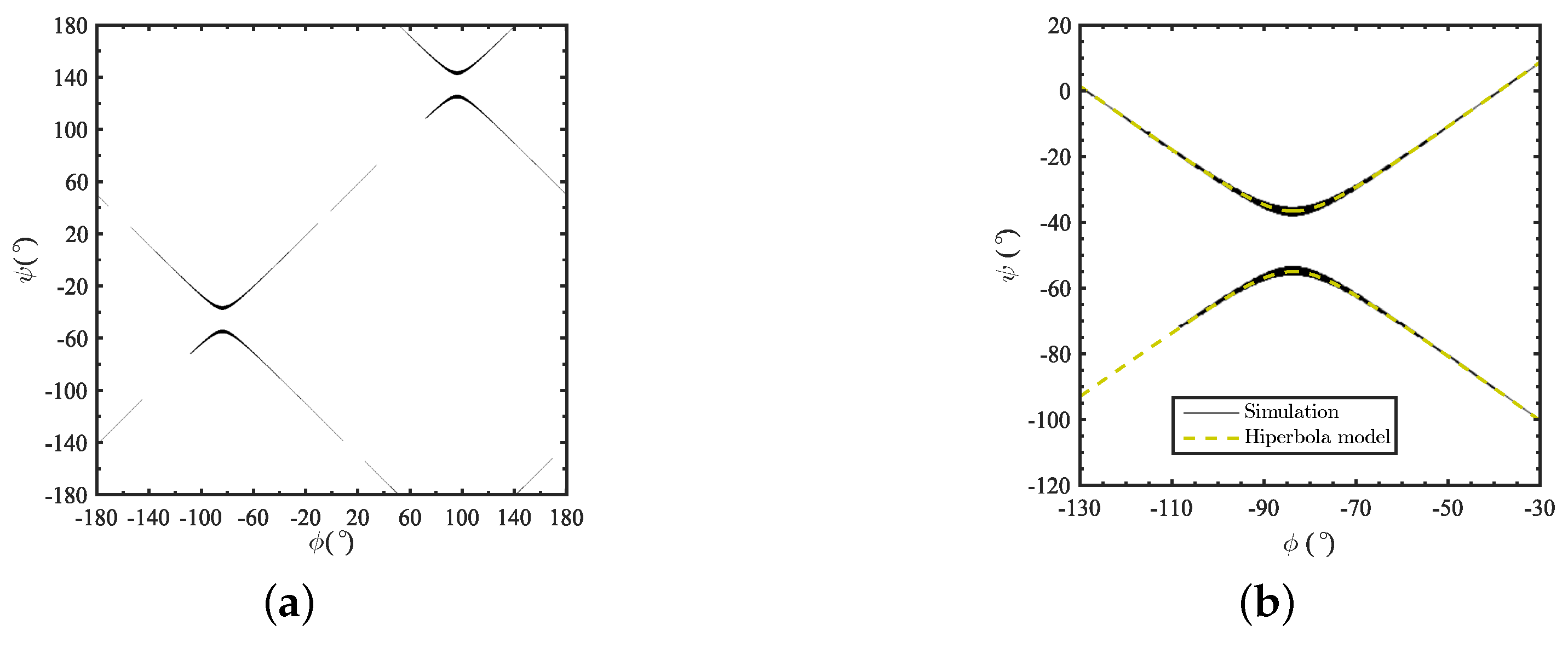
However, if the prescribed TZs are distributed asymmetrically along the network in a ladder topology, the phase terms ${\theta }_{11}\left(s\right)$, ${\theta }_{22}\left(s\right)$ are expected to be different in order to comply with the extraction of all homogeneous admittance inverters in the network. In other words, if the TZs of the filter are asymmetrically distributed, asymmetric characteristic polynomials are required. 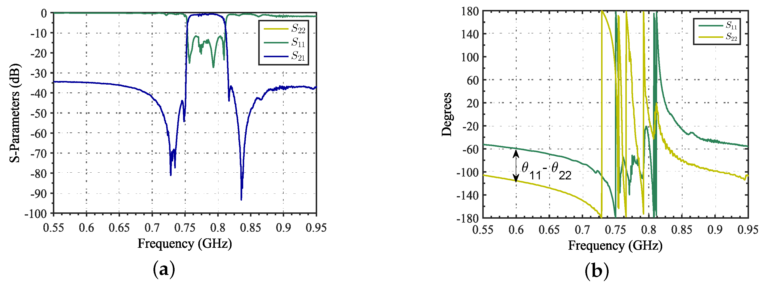For the sake of clarity, in Figure 4a there is a measure of a B28Rx seventh-order filter with an asymmetrical TZs distribution. It is observable in Figure 4b that input and output phases are not equal. This occurrence can be clearly seen in the OoB regions, where the difference between ${\theta }_{11}\left(s\right)$ and ${\theta }_{22}\left(s\right)$ is directly the offset between both traces.

In this section, the phenomenon has been addressed from the admittance redistribution which is equivalent to the modification of the phase of the characteristic polynomials (defined symmetric by nature). However, as it will be further discussed in the next section, this solution can be understood as a particular case belonging to a more general solutions map provided by the use of asymmetric polynomials.

Figure 4. Magnitude (a) and phase (b) response of a 7th-order B28-Rx filter with a clearly differentiated input and output phases in the out-out-band region.

Figure 4. Magnitude (a) and phase (b) response of a 7th-order B28-Rx filter with a clearly differentiated input and output phases in the out-out-band region.

3. Asymmetrical Polynomial Definition

The procedure for the definition of the asymmetrical polynomials to deal with asymmetrically distributed TZs filter networks is based on the work in [17]. The relation between modified scattering parameters and Chebyshev characteristic polynomials is given by:

$$\begin{array}{c}\hfill \begin{array}{c}\begin{array}{c}{S}_{11}\left(s\right)={\displaystyle \frac{F_{11m}\left(s\right)}{E_m\left(s\right)}},S_{22}\left(s\right)={\displaystyle \frac{F_{22m}\left(s\right)}{E_m\left(s\right)}},\hfill \\ \\ S_{21}\left(s\right)=S_{12}\left(s\right)={\displaystyle \frac{P_m\left(s\right)}{E_m\left(s\right)}}.\hfill \end{array}\hfill \end{array}\end{array}$$

(9)

where the subscript m refers to modified characteristic polynomials that are defined as follows:

$$\begin{array}{c}\hfill \begin{array}{c}{F}_{11m}\left(s\right)={\displaystyle \frac{F\left(s\right)}{{\epsilon }_R}}\sqrt{\frac{\Psi }{\Phi }},\hfill \\ \\ F_{22m}\left(s\right)={\displaystyle \frac{{(-1)}^N{F}^{*}\left(s\right)}{{\epsilon }_R}}\sqrt{\frac{\Phi }{\Psi }},\hfill \\ \\ E_m\left(s\right)={\displaystyle \frac{E\left(s\right)}{\sqrt{\Psi \Phi }}}.\hfill \end{array}\end{array}$$

(10)

The parameters $\Psi$ and $\Phi$ are complex constants which absolute value is $|\Psi |=|\Phi |=1$. With the angles associated with these new variables ($\psi ,\varphi$), the phase of $F_{11m}$ and $F_{22m}$ can be modified. Both phase terms are bounded together and linked to the phase of $E_m\left(s\right)$.

$$\begin{array}{ccc}\hfill \Psi =e^{j\psi }& ,\hfill & \hfill \Phi =e^{j\varphi }.\end{array}$$

(11)

The lowpass prototype network synthesis is carried out by means of successive extractions from the $\left[ABCD\right]$ polynomial matrix as described in [4,12]. The procedure requires N recursive steps. For a two-port network having the terminals normalized to unity, the network $\left[ABCD\right]$ matrix is built as follows:

$$\begin{array}{c}\left[ABCD\right]={\displaystyle \frac{1}{jP\left(s\right)/\epsilon }}\left[\begin{array}{cc}A\left(s\right)& B\left(s\right)\\ C\left(s\right)& D\left(s\right)\end{array}\right]\hfill \end{array}$$

(12)

The extracted pole sections are made of a non-resonant node and resonant node pairs (NRN-RN). At each iteration k, the extraction will be performed at a normalized finite frequency $j{\Omega }_i^k$, being $k=1...N$ the iteration number, and $i=1...N$ the resonator position. The extracted elements must be removed from the ABCD matrix in (12) which is updated after every step. Using the classic two-port [S] matrix to $\left[ABCD\right]$ matrix transformation formulas with normalized characteristic impedance, the polynomials A(s), B(s), C(s), and D(s) in (12) may be directly expressed in terms of the coefficients of modified characteristic polynomials $F_{11m}\left(s\right)$, $F_{22m}\left(s\right)$ and $E_m\left(s\right)$:

$$\begin{array}{c}\hfill \begin{array}{c}A\left(s\right)={\displaystyle \frac{(E_m\left(s\right)+F_{11m}\left(s\right))(E_m\left(s\right)-F_{22m}\left(s\right))+P_m^2\left(s\right)}{2E_m\left(s\right)}},\hfill \\ \\ B\left(s\right)={\displaystyle \frac{(E_m\left(s\right)+F_{11m}\left(s\right))(E_m\left(s\right)+F_{22m}\left(s\right))-P_m^2\left(s\right)}{2E_m\left(s\right)}},\hfill \\ \\ C\left(s\right)={\displaystyle \frac{(E_m\left(s\right)-F_{11m}\left(s\right))(E_m\left(s\right)-F_{22m}\left(s\right))-P_m^2\left(s\right)}{2E_m\left(s\right)}},\hfill \\ \\ D\left(s\right)={\displaystyle \frac{(E_m\left(s\right)-F_{11m}\left(s\right))(E_m\left(s\right)+F_{22m}\left(s\right))+P_m^2\left(s\right)}{2E_m\left(s\right)}},\hfill \\ \\ Pm\left(s\right)={\displaystyle \frac{P\left(s\right)}{\epsilon }}.\hfill \end{array}\end{array}$$

(13)

Adopting the equations in (13) the extraction process can be carried out as usual [12]. If $\Psi$ and $\Phi$ are properly defined, it is expected that the extraction process will yield the last inverter $J_{N+1}$ to a unitary value. However, the definition of the asymmetrical polynomial depends directly on the chosen values for $\Psi$ and $\Phi$.

4. Phase Determination

With the aim to find out the definition of $\psi$ and $\varphi$ that yields $|J_{N+1}|=1$, a space map of solutions has been obtained by sweeping both variables, i.e., input and output phase correction, and carrying the extraction of elements in every case. The space map of solutions results in a particular geometric pattern that, as it will be developed through this section, will be different for odd- and even-order networks. For odd-order filters, the suitable phase values are like an equilateral hyperbola while they describe an ellipse in the case of even-order filters. Although both are different, they belong to the same group of geometric shapes, conic sections. They can be defined as non-degenerate curves shape that can be obtained when a plane intersects one or two right circular cones [18]. They can be differentiated by the eccentricity e, a constant value that characterizes the shape of a curve. When it is greater than 1, the geometric shape corresponds to a hyperbola, conversely if $0<e<1$, the result is an ellipse. In the following, the method to find all suitable phase values for both cases is described.

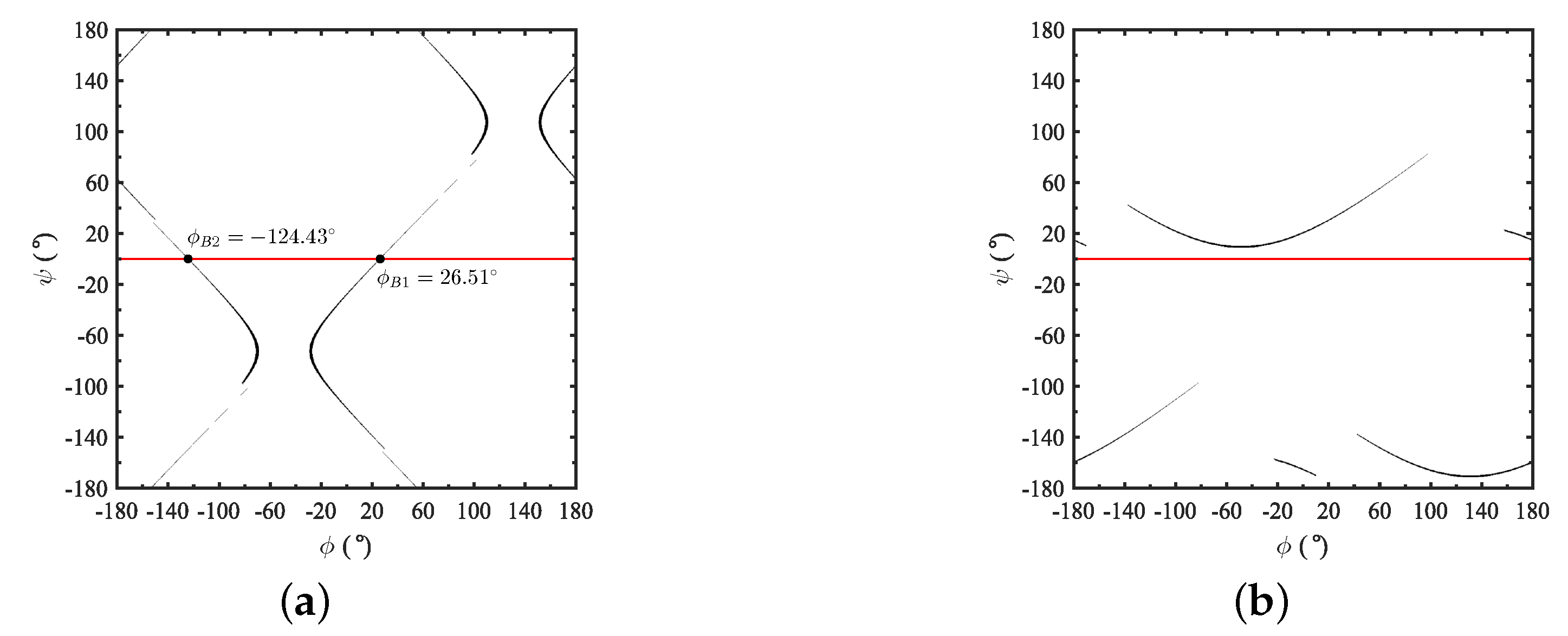
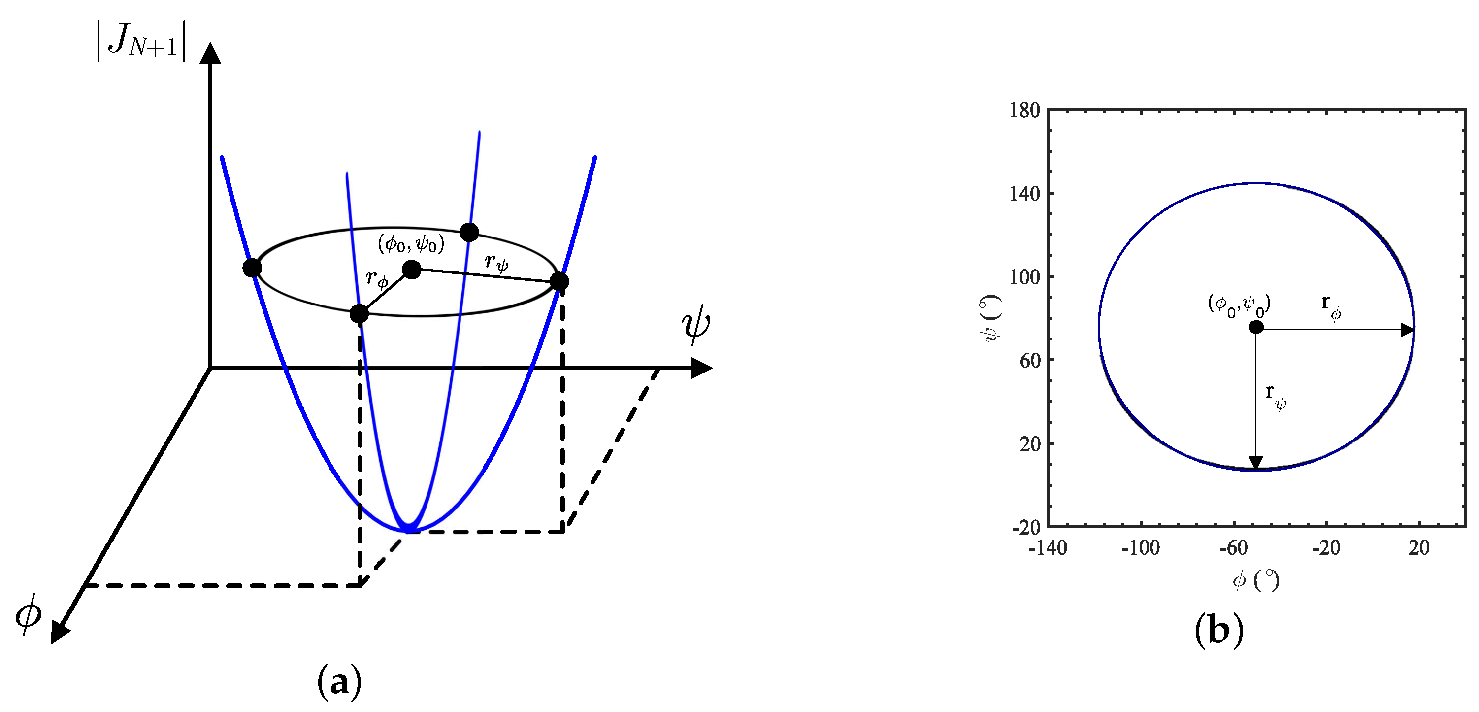
4.1. Odd-Order Ladder Filters

To fully characterize a network, for each TZs array ${\Omega }_{tzi}$, a double phase sweep has been conducted doing $n_{\psi }\times n_{\varphi }$ complete circuital extractions from the network ABCD matrix, where the effect is located to the last admittance inverter, being $n_{\psi }$ and $n_{\varphi }$ the individual number of sweeps in $\psi$ and $\varphi$ variables, respectively.

The $J_{N+1}$ value evolution is obtained as a function of $(\psi ,\varphi )$. Both parameters have been swept in a range from $-{180}^{\circ }$ to ${180}^{\circ }$. The values for the pair $(\psi$, $\varphi )$ yielding $J_{N+1}=1\pm 0.001$ describe a map that can be fitted with the parametric equation of a conjugate hyperbola as shown in Figure 5a,b, respectively.

A hyperbola can be completely defined by four parameters: the hyperbola type (horizontal or vertical), the two slant asymptotes, the origin locus, and the distance from it to the vertex of one branch ($\alpha$). Whereas it is equilateral in any case, its slant asymptotes have a slope 1 at $\psi =\pm \varphi$. Through observation, it has been discerned that unitary $J_{N+1}(\varphi ,\psi )$ describes an equilateral hyperbola-like shape which origin location coincides with ${\psi }_0={\theta }_{11}\left(j{\omega }_1\right)$, ${\varphi }_0={\theta }_{22}\left(j{\omega }_N\right)$, given by:

$$\begin{array}{cc}\hfill & {\left.{\theta }_{11}\left(s\right)={\displaystyle \frac{F\left(s\right)}{E\left(s\right)}}\right|}_{s=j{\omega }_1}\hfill \end{array}$$

(14a)

$$\begin{array}{cc}\hfill & {\left.{\theta }_{22}\left(s\right)={\displaystyle \frac{F\left(s\right)}{E\left(s\right)}}\right|}_{s=j{\omega }_N}\hfill \end{array}$$

(14b)

The general equation for equilateral hyperbolas is:

$$\begin{array}{c}\hfill {\displaystyle \frac{{(\varphi -{\varphi }_0)}^2-{(\psi -{\psi }_0)}^2}{{\alpha }^2}}=\pm 1.\end{array}$$

(15)

If the LHS of Equation (15) is negative, the hyperbola aperture is vertical, and horizontal otherwise. The hyperbola type is determined by the $|J_{N+1}|$ value that results from the network synthesis considering $\psi =0^{\circ }$, $\varphi =0^{\circ }$. If $|J_{N+1}|<1$ the hyperbola is vertical and horizontal when $|J_{N+1}|>1$.

The value of $|J_{N+1}|$ can be only known after performing a whole network extraction. In filters which TZs distribution presents internal symmetry and different outer TZs such as ${\Omega }_{tz}=\{{\Omega }_1,{\Omega }_2,{\Omega }_3,{\Omega }_2,{\Omega }_4\}$, the hyperbola type could be recognized a priori from the absolute value of the input and output phases $|{\psi }_0|$ and $|{\varphi }_0|$ obtained using (14). If $|{\psi }_0|>|{\varphi }_0|$, the hyperbola is vertical and horizontal if $|{\psi }_0|<|{\varphi }_0|$. However, this behavior can only be observed in such a case. These phase terms are obtained using the normalized frequency of the first and last TZ of the network. A phase term is greater as the TZ is closer to the center frequency and vice versa. It also should be noted in Figure 5a, that the both hyperbola-like shapes present periodicity every $\pm {180}^{\circ }$ degrees in ${\psi }_0$ and ${\varphi }_0$ directions regardless its aperture.

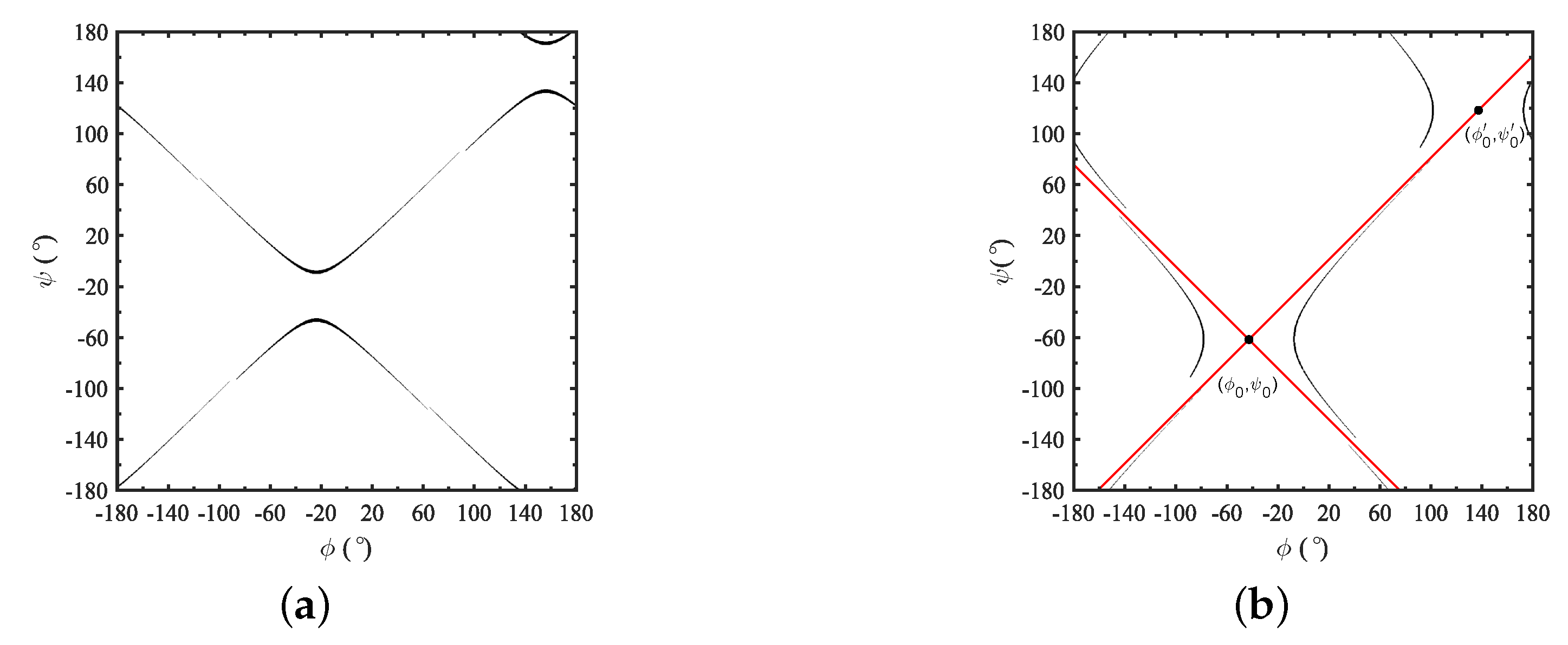
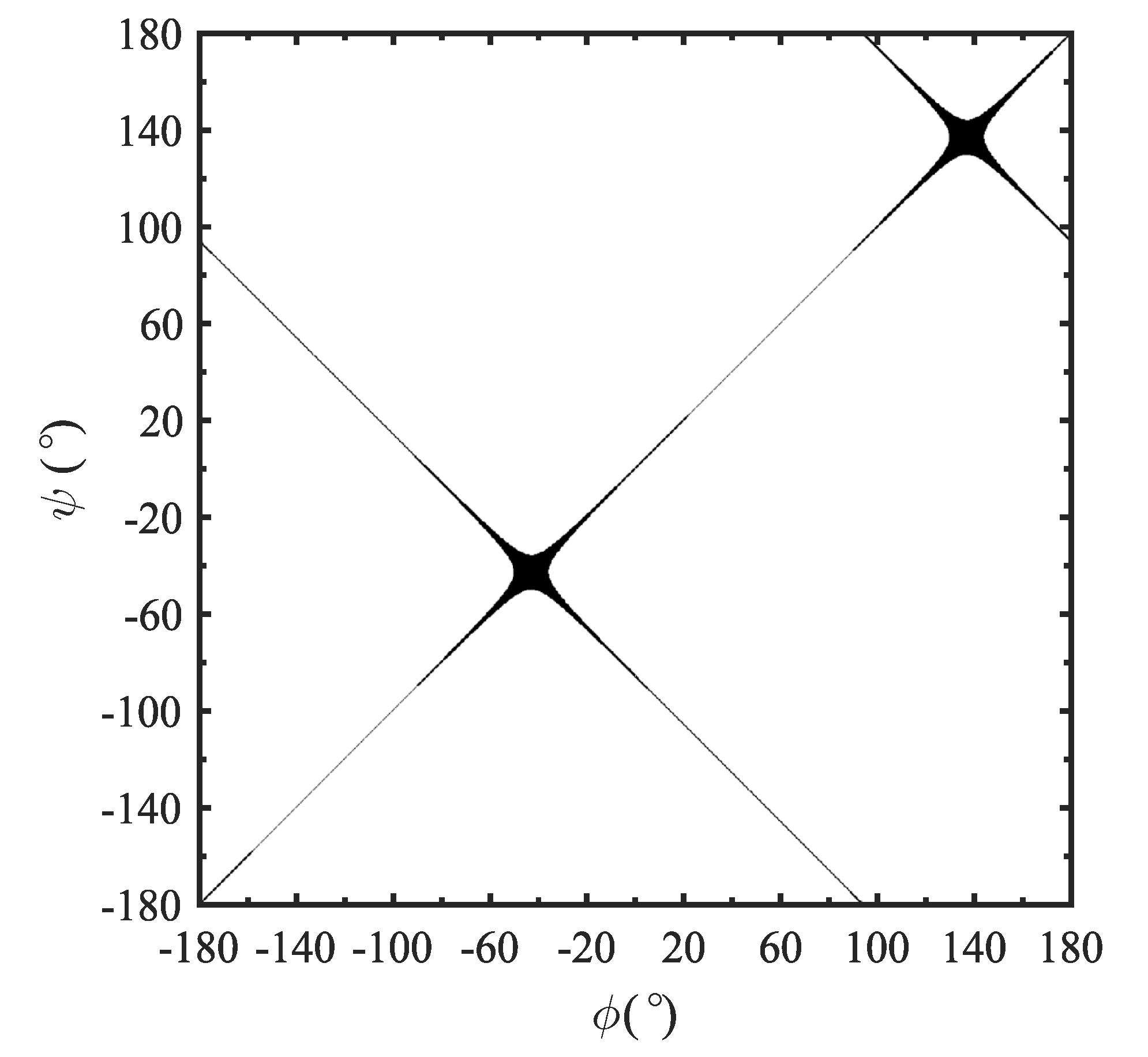
Apart from these two orientation types, there is also a third possibility, filters with TZs distribution in such a way that it is achieved $|J_{N+1}|=1$ before correcting the polynomial phases. Here, the vertices of both branches are located in the origin of the hyperbola, as shown in Figure 6. This situation is given, but not exclusively, when the TZs are symmetrically allocated along the network. As expected, the asymptote with positive and negative slope are given by $\psi =(\varphi -{\varphi }_0)+{\psi }_0$ and $\psi =-(\varphi -{\varphi }_0)+{\psi }_0$, respectively.

The vertices cannot be inferred directly from the function representation in any of the previous cases. The calculation is carried out by an indirect approach that it will be described in Section 5.1.

In the following, they are going to be under discussion to illustrate in more detail the three possible results. In the first two cases, the horizontal and vertical hyperbolas are shown; the third case explores filters with TZs distribution which $|J_{N+1}|=1$ with the initial starting set-up ($\psi =\varphi =0$). Finally, the method used to obtain the vertex location $V_h$ is described.

Hyperbola Types

The analysis of the three cases has been done following the same procedure. First, a network synthesis is done without modifying the polynomials to obtain the $J_{N+1}$ used to identify the hyperbola type. Then, the phase sweep is carried out and the results are plotted.

Let us consider first a 5th-order lowpass fully canonical filter with a TZs set ${\Omega }_{tz1}=\{2.6,-1.6,2.6,-2.5,3\}$ rad/s and $R{L}_1=10$ dB. An initial network synthesis yields $|J_{N+1}|=1.005503$. As the admittance inverter is greater than one, the hyperbola is horizontal as the one in Figure 5a. The center, calculated using (14), is located at ${\psi }_0={\theta }_{11}=-{27.8209}^{\circ }$, ${\varphi }_0={\theta }_{22}=-{23.7531}^{\circ }$.

For the vertical case, a 5th-order lowpass fully canonical filter with a set of TZs ${\Omega }_{tz2}=\{1.4,-1.7,2.6,-2,1.8\}$ rad/s and $R{L}_2=10$ dB is considered. An initial network synthesis yields $|J_{N+1}|=0.878566$, the admittance inverter is lower than 1, meaning that the hyperbola is vertical as shown in Figure 5b. The center is located in ${\psi }_0={\theta }_{11}=-{61.5988}^{\circ }$, ${\varphi }_0={\theta }_{22}=-{42.7635}^{\circ }$.

As seen in Figure 5a, the continuity in the function is interrupted at some points. This discontinuity occurs when traces cross the asymptotes of the hyperbolic response. As mention before, the hyperbolas shows a periodicity every $\pm {180}^{\circ }$; the traces that appears after the end of the interrupted traces belongs to another hyperbola in other region on the map. A large number of realizations has been carried out obtaining a margin of $\pm {45}^{\circ }$ for $\psi$ and $\varphi$ around the origin point, where the continuity is assured.

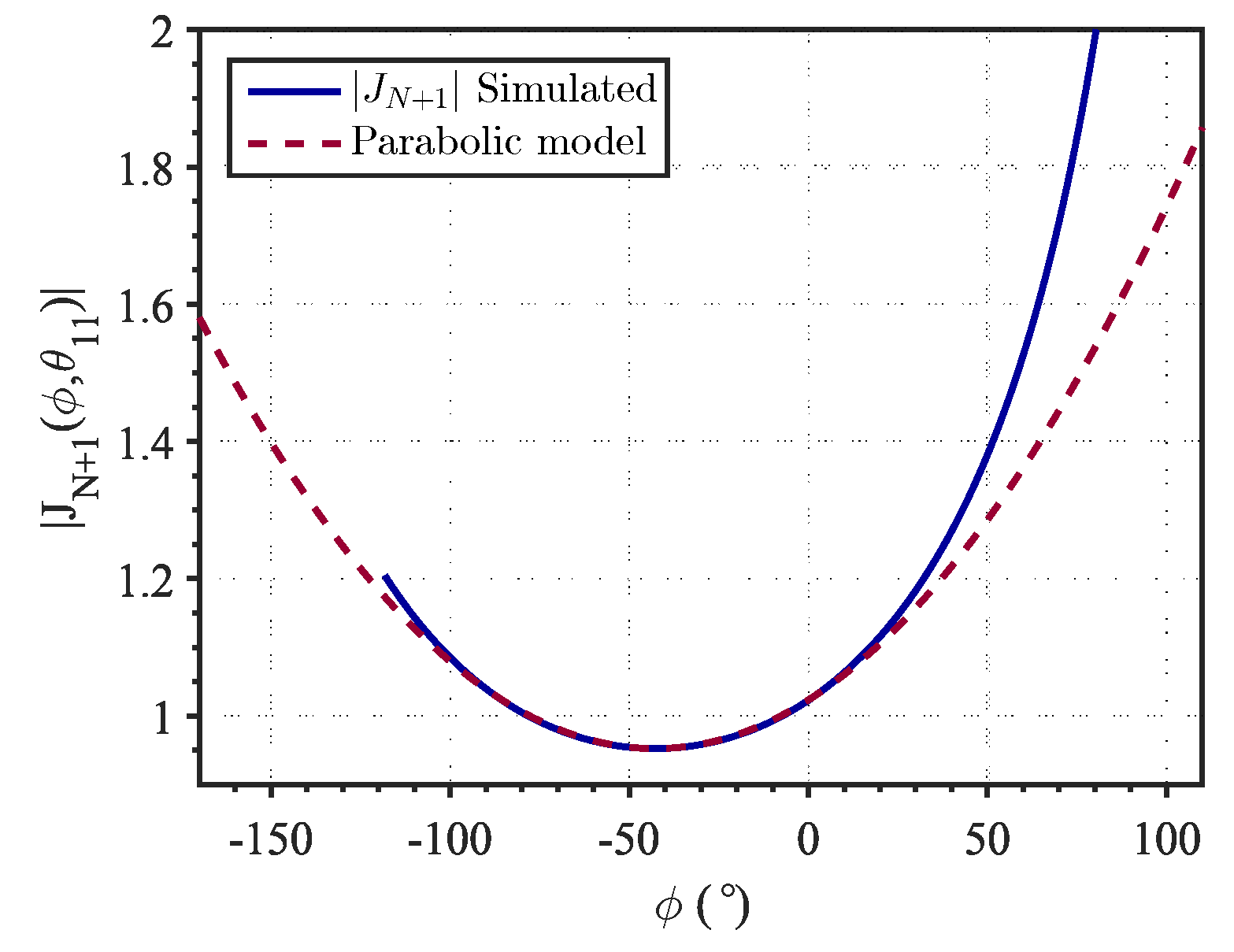
Considering the absolute value of the uneven admittance inverter as a measure of the asymmetry of the values in a certain TZs distribution, as $|J_{N+1}|$ tends to move away from unity, the further the hyperbola branches are.

The third case is given in filters with symmetric TZs distribution. Let us consider a 5th-order lowpass fully canonical filter with a TZs set ${\Omega }_{tz3}=\{1.8,-2,2.6,-2,1.8\}$ rad/s and $R{L}_3=10$ dB. An initial network synthesis yields $|J_{N+1}|=1$. As shown in Figure 6, the sweep yields two slopes that cross in the center point. That is, the valid pairs $\varphi$, $\psi$ are those that lie directly over the asymptotes. It must be also highlighted that in this case, the area in which $|J_{N+1}|=1\pm 0.001$ is more extensive than previous cases. This leads to less sensitive networks from the point of view of input/output phase shifts. This special case corresponds to a degenerate conic section, described as two intersecting lines [19], which particular mathematical expression is

$$\begin{array}{c}\hfill {\displaystyle \frac{{(\varphi -{\varphi }_0)}^2-{(\psi -{\psi }_0)}^2}{{\alpha }^2}}=0.\end{array}$$

(16)

Effectively, it can be observed in Figure 6 that there are identified pairs of angles ($\varphi$, $\psi$) suited to correct the input/output phase of the network. Moreover, as the solution is not unique, the designer has the chance to select that pair of phase values which leads to obtaining $|J_{N+1}|$=1, but at the same time considering other phase requirements as it could be the case of avoiding loading effects in the design of duplexers or multiplexers [6].

Figure 6. Phase sweep plot when the distance to the vertex is zero. The black trace represents those combinations of $\psi$, $\varphi$ that yields $|J_{N+1}|=1$. For illustration purpose all $|J_{N+1}|$ values that fit in $1\pm 0.001$ have been plotted.

Figure 6. Phase sweep plot when the distance to the vertex is zero. The black trace represents those combinations of $\psi$, $\varphi$ that yields $|J_{N+1}|=1$. For illustration purpose all $|J_{N+1}|$ values that fit in $1\pm 0.001$ have been plotted.

When the network is synthesized applying the phase correction using ($\varphi$, $\psi$) corresponding to one of the vertices, one of the reactive input/output elements will be zero because one of the phase terms cancels the input or output phase. If the hyperbola is vertically orientated $\psi ={\psi }_0$, which is ${\theta }_{11}$, the new input phase will be zero and no reactive element at the source port $B_S$ is necessary [1]. Conversely, if the hyperbola is found to be horizontal, the reactive element at the output port will be zero. Besides, if different valid ($\varphi ,\psi$) pairs are used, none of the input/output reactive elements will be null.

4.2. Relationship between the Phase Map and the Admittance Redistribution Method

As was described in Section 2, the described method to equalize the inverter values in the main-line by an admittance redistribution modifies ${\theta }_{22}\left(s\right)$ without altering ${\theta }_{11}\left(s\right)$. Hence, this is equivalent to pre-modify the characteristic polynomials before the circuital extraction with $\psi =0$ and certain value for $\varphi$.

The filter used to exemplify the admittance redistribution with ${\Omega }_{Bk}$ TZs showed two values for $B_L$, positive or negative depending on the sign of the square root. These solutions lead to two different circuit elements or, equivalently, two additive output phase terms ${\varphi }_{B1}$ and ${\varphi }_{B2}$. Before the redistribution, $B_L=-0.4553$ and the phase term is ${\varphi }_0=-{48.96}^{\circ }$. Once the redistribution is done, $B_L^{\prime }=\pm 0.7739$, that yields ${\varphi }_0^{\prime }=\pm {75.4726}^{\circ }$. Therefore, the additive phases can be obtained as

$$\begin{array}{cc}\hfill {\varphi }_{B1}& ={\varphi }_0+\left|{\varphi }_0^{\prime }\right|={26.51}^{\circ },\hfill \end{array}$$

(17a)

$$\begin{array}{cc}\hfill {\varphi }_{B2}& ={\varphi }_0-\left|{\varphi }_0^{\prime }\right|=-{124.43}^{\circ }.\hfill \end{array}$$

(17b)

In the original synthesized filter, the last admittance inverter is $|J_6|=0.8689$, lower than 1. Thus, a double phase sweep of the characteristic polynomials describes the vertical hyperbola shown in Figure 7a. It can be noted that there are two points cutting the hyperbola (solutions for $|J_{N+1}|$=1) at $\psi =0$, and these two values correspond with ${\varphi }_{B1}$ and ${\varphi }_{B2}$. This result reveals that the circuital transformation done by the admittance redistribution is actually a particular case within the hyperbola.

On the other hand, a particular TZs distribution may lead to a situation in which the admittance distribution is not possible unless impedance mismatch is allowed as it was the case with TZs ${\Omega }_{Ck}=\{1.8,-1.16,1.8,-2,2.5\}$. The double phase sweep of this filter yields the phase map in Figure 7b. It can be observed that no point is cutting the hyperbola at $\psi$ = 0. In other words, there is no additive output phase $\varphi$ that can correct the last admittance inverter if the input phase term $\psi$ is zero. This brings to light the cause of the admittance redistribution method applicability limitation, and reinforce the necessity of the asymmetrical polynomial definition in such cases.

From both phase maps in Figure 7 it can be concluded that in all networks with $|J_{N+1}|<1$ (vertical hyperbola), the redistribution is always possible because there exist a cutting point at $\psi =0$ in both branches. However, for those networks with $|J_{N+1}|>1$ (horizontal hyperbola), it may occur that no branches crosses the line at $\psi =0$. In this case, to equalize the uneven inverter is necessary to change, at least, the input phase with a non-zero $\psi$ value.

4.3. Even-Order Ladder Filters

A symmetric distribution of the TZ in odd-order networks can be achieved by having the same resonant frequencies at both halves of the network, considering the central resonator as an axis of symmetry. Hence, even-order filters do not posses symmetry under these terms and the unitary admittance inverters can only be achieved, without any phase correction, by a careful selection of TZs and RL values. For example, with the network with TZs ${\Omega }_{Dk}=\{2.5,-1.3,1.5,-2.64,2,-1.86\}$ rad/s and $RL=20$ dB, which network parameters are listed in

Table 3. Extracted elements of the 6th-order filter prototype with a ${\Omega }_{Dk}$ TZs distribution.

Parameters	${\mathit{B}}_{\mathit{k}}$	${\mathit{b}}_{\mathit{k}}$	${\mathit{J}}_{\mathit{rk}}$
Res. 1	−1.6233	−2.50	2.091
Res. 2	1.2539	1.30	0.97845
Res. 3	−2.4661	−1.50	1.827
Res. 4	3.1101	2.64	2.9667
Res. 5	−3.4831	−2.00	2.4392
Res. 6	1.2111	1.86	1.2928
$B_S$	−0.4460
$B_L$	0.6775

, the admittance inverters are $J_k=\{1,-1,1,-1,1,-1,1\}$.

In any event, the unique geometric shape that defines the input and output phases ($\Psi ,\Phi$) providing an unitary admittance inverter for even-order filters is an ellipse. To illustrate the phenomenon, let us consider a 4th-order fully canonical filter with a TZs ${\Omega }_{Ek}=\{-1.8,1.6,-2,2.5\}$ and RL $=20$ dB, with the network parameters in

Table 4. Extracted elements of the 4th-order filter prototype with a ${\Omega }_{Ek}$ TZs distribution.

Parameters	${\mathit{B}}_{\mathit{k}}$	${\mathit{b}}_{\mathit{k}}$	${\mathit{J}}_{\mathit{rk}}$
Res. 1	0.9234	1.8000	1.108
Res. 2	−2.3310	−1.6000	1.6192
Res. 3	1.8854	2.0000	1.8385
Res. 4	−2.4007	−2.5000	2.3224
$B_S$	0.7782
$B_L$	−0.4700

and S-parameters in Figure 8a. The synthesis yields $J_k=\{1,-1,1,-1,1.1593\}$. The result of the sweep reveals the ellipses in Figure 8b.

In this case, the location of the origin at ${\psi }_0$ and ${\varphi }_0$ can be also determined using (14), and periodicity in the ellipse every $\pm {180}^{\circ }$ in both axis ($\psi$ and $\varphi$) is observed again. The origin in this case is located at (${\psi }_0=-{50.3462}^{\circ }$, ${\varphi }_0={75.7811}^{\circ }$). However, unlike the odd-order filters, the even-order do not show any variation in shape.

Besides, it can be noted that the black trace in Figure 8b never cuts $\psi =0^{\circ }$. That is, even-order filters may be susceptible to not have any output additive phase term $\varphi$ that can provide a unitary admittance inverter $|J_{N+1}|$ without modifying the input phase. In consequence, it may exist network configurations in which the admittance redistribution method is not applicable either.

The ellipse can be completely characterized by three parameters: the center location, the major radius and minor radius, where the general equation is

$${\displaystyle \frac{{(\varphi -{\varphi }_0)}^2}{r_{\varphi }^2}}-{\displaystyle \frac{{(\psi -{\psi }_0)}^2}{r_{\psi }^2}}=1$$

(18)

To keep coherence with the rest of the text, the radii will be referred as $r_{\psi }$ and $r_{\varphi }$ in function of the axis in which they are defined instead of their length from the center.

5. Fast Estimation of the Phase Maps

Performing a phase map for every network is a time-consuming task, doing a sweep from $-{180}^{\circ }$ to ${180}^{\circ }$ in both $\psi$ and $\varphi$ with a good precision requires about ${10}^6$ full extractions. In this section, a fast and systematic method to obtain an accurate model for both shapes, the hyperbola and the ellipse, is described.

The proposed methods are generic so that makes it unnecessary to perform the phase exploration each time, enabling achieving a proper solution directly with a low computational cost.

5.1. Hyperbolic Model Estimation

As mentioned earlier, to model a hyperbola four parameters are required: the hyperbola type (horizontal or vertical), the two slant asymptotes, the origin locus and the distance from it to the vertex of one branch. All of them can be obtained from the network parameters except the vertices. The vertex is the point at each branch closest to the center. To find its value, an indirect approach has been employed.

Since both vertices belong to the hyperbola, they will provide $|J_{N+1}|=1$. A phase sweep has been carried out along the transverse axis, the line going from one vertex to the other. If it is a vertical hyperbola, the transverse axis is defined in $\varphi$ axis, being also the sweeping parameter. Meanwhile, $\psi$ is fixed and set to ${\psi }_0={\theta }_{11}$. In the horizontal hyperbola case, $\psi$ is the sweeping parameter and ${\varphi }_0={\theta }_{22}$. The traced curve is accurately described by a geometric parabolic function that is continuous within the range of interest given by (19) and (20) for the vertical and horizontal hyperbola case, respectively. To avoid confusion, the parabola and hyperbola vertices have been denoted as $V_p$ and $V_h$, respectively.

$$\begin{array}{c}\hfill \varphi =\pm ({180}^{\circ }-|{\theta }_{11}\left|\right),\end{array}$$

(19)

$$\begin{array}{c}\hfill \psi =\pm ({180}^{\circ }-|{\theta }_{22}\left|\right).\end{array}$$

(20)

For the vertical hyperbola case, the vertex of the parabola is identified by $V_p({\varphi }_0,|J_{N+1}({\varphi }_0,{\psi }_0)\left|\right)$. At equal distance to the vertex there are two $|J_{N+1}|$ values that are unitary and these points meet with the hyperbola vertices. Although the curve is not exactly a parabola, the approximation is valid for range close to the vertex $V_p$, because is where the solution usually is, and $V_p$ does not takes values far from one. The equation is defined as follows:

$${(\varphi -{\varphi }_0)}^2=4p\left(\right|J_{N+1}(\varphi ,{\psi }_0)|-|J_{N+1}({\varphi }_0,{\psi }_0)\left|\right),$$

(21)

where p is a constant that controls the parabola steepness. It can be obtained as:

$$p={\displaystyle \frac{{(\varphi -{\varphi }_0)}^2}{4\left(\right|J_{N+1}(\varphi ,{\psi }_0)|-|J_{N+1}({\psi }_0,{\varphi }_0)\left|\right)}}.$$

(22)

The $\varphi$ value for calculating p should be chosen close to the vertex $V_p$ to achieve an accurate approximation to the curve steep. Of course, higher polynomial fit can be successfully used to increase the range and accuracy of the approximation, but based on the conducted experiments, the parabolic model is computationally faster, accurate enough, and facilitates the understanding. The hyperbola vertices can be obtained from (21) by setting $|J_{N+1}(\varphi ,{\psi }_0)|=1$ and solving for $\varphi$ that are the angles where the vertices are located.

$$\varphi ={\varphi }_0\pm 2\sqrt{p(1-|J_{N+1}({\varphi }_0,{\psi }_0)\left|\right)}$$

(23)

Using Equation (23), the vertices points of a vertical hyperbola are $V_h({\varphi }_0\pm \alpha ,{\psi }_0)$, where $\alpha$ is define as

$$\alpha =2\sqrt{p(1-|J_{N+1}({\varphi }_0,{\psi }_0)\left|\right)}.$$

(24)

Considering the filter used in the previous section with TZs ${\Omega }_{tz1}$, the vertices are located at $\varphi ={\varphi }_0\pm {35.04}^{\circ }$ and $\psi ={\psi }_0$. As shown in Figure 9, the approximation is accurate around the parabola vertex. Analogously, when the hyperbola is horizontal, the parabola function equations are calculated, as follows:

$$\begin{array}{cc}\hfill {(\psi -{\psi }_0)}^2& =4p\left(\right|J_{N+1}({\varphi }_0,\psi )|-|J_{N+1}({\varphi }_0,{\psi }_0)\left|\right),\hfill \end{array}$$

(25a)

$$\begin{array}{cc}\hfill p& ={\displaystyle \frac{{(\psi -{\psi }_0)}^2}{4\left(\right|J_{N+1}({\varphi }_0,\psi )|-|J_{N+1}({\varphi }_0,{\psi }_0)\left|\right)}},\hfill \end{array}$$

(25b)

$$\begin{array}{cc}\hfill \psi & ={\psi }_0\pm \alpha .\hfill \end{array}$$

(25c)

Finally, the vertices points are defined as $V_h({\varphi }_0,{\psi }_0\pm \alpha )$.

5.2. Illustrative Synthesis Example

A Chebyshev 7th-order fully canonical filter with an asymmetric TZs distribution is presented to demonstrate the accuracy of the proposed method. The transmission zeros are ${\Omega }_{tz}=\{2.4,-2.1,1.7,-1.8,2,-1.7,1.5\}$ rad/s and $RL=18$ dB. All characteristic polynomials are listed in Table 5.

The lowpass prototype filter resulting from the network synthesis is like the one depicted in Figure 1 with $N=7$. The extracted parameters are shown in Table 6 leading to the transmission and reflection response, in the lowpass domain, depicted in Figure 10. In this case, the extracted uneven admittance inverter is $|J_{N+1}|=1.2405$, meaning that the hyperbola is horizontal as shown in Figure 11a. The center of the hyperbola, obtained with (14), is located in $C(\varphi =-83.6889,\psi =-{45.814}^{\circ })$, ${\theta }_{22}$ and ${\theta }_{11}$, respectively.

Figure 10. Lowpass transmission and reflection response of the extracted network.

Figure 10. Lowpass transmission and reflection response of the extracted network.

Table 5. Characteristic polynomial coefficients for the filter with ${\Omega }_{tz}$ TZs distribution and $RL=$ 18 dB for different additional phase terms.

Initial Characteristic Polynomials
deg.	$\mathit{P}\left(\mathit{s}\right)$			$\mathit{E}\left(\mathit{s}\right)$			${\mathit{F}}_{\mathbf{11}}\left(\mathit{s}\right)$			${\mathit{F}}_{\mathbf{22}}\left(\mathit{s}\right)$
0	78.6542			0.1852 − 0.1290j			−0.0161j			−0.0161j
1	43.3847			0.8449 − 0.4246j			0.1470			0.1470
2	70.4446j			1.9944 − 0.8376j			−0.2183j			−0.2183j
3	37.6407			3.3274 − 1.0378j			1.0165			1.0165
4	20.7380j			3.6860 − 1.0261j			−0.5080j			−0.5080j
5	10.7200			3.4792 − 0.5680j			1.8598			1.8598
6	2.0000j			1.7997 − 0.3115j			−0.3115j			−0.3115j
7	1			1			1			1
Modified Polynomials by$\mathit{\varphi }=-{\mathbf{83.6889}}^{\circ }$, $\mathit{\psi }=-{\mathbf{36.6610}}^{\circ }$
deg.	${\mathit{E}}_{\mathit{m}}\left(\mathit{s}\right)$				${\mathit{F}}_{\mathbf{11}\mathit{m}}\left(\mathit{s}\right)$				${\mathit{F}}_{\mathbf{22}\mathit{m}}\left(\mathit{s}\right)$
0	0.2040 + 0.0965j				0.0064 − 0.0147j				0.0064 − 0.0147j
1	0.7885 + 0.5218j				0.1348 + 0.0586j				0.1347 + 0.0586j
2	1.7186 + 1.3137j				0.0871 − 0.2001j				0.0870 − 0.2001j
3	2.5552 + 2.3705j				0.9321 + 0.4056j				0.9321 + 0.4055j
4	2.7234 + 2.6874j				0.2027 − 0.4658j				0.2026 − 0.4658j
5	2.2232 + 2.7359j				1.7053 + 0.7420j				1.7053 + 0.7420j
6	1.1653 + 1.4064j				0.1243 − 0.2856j				0.1242 − 0.2855j
7	0.4974 + 0.8675j				0.9170 + 0.3990j				0.9169 + 0.3989j
Modified Polynomials by$\mathit{\varphi }=-{\mathbf{53.51}}^{\circ }$, $\mathit{\psi }=-{\mathbf{14.18}}^{\circ }$
deg.	${\mathit{E}}_{\mathit{m}}\left(\mathit{s}\right)$				${\mathit{F}}_{\mathbf{11}\mathit{m}}\left(\mathit{s}\right)$				${\mathit{F}}_{\mathbf{22}\mathit{m}}\left(\mathit{s}\right)$
0	0.2257 − 0.0040j				0.0054 − 0.0151j				0.0054 − 0.0151j
1	0.9382 + 0.1179j				0.1384 + 0.0495j				0.1384 + 0.0494j
2	2.1230 + 0.4152j				0.0734 − 0.2055j				0.0734 − 0.2055j
3	3.3415 + 0.9912j				0.9572 + 0.3421j				0.9572 + 0.3420j
4	3.6328 + 1.2007j				0.1710 − 0.4784j				0.1709 − 0.4783j
5	3.2060 + 1.4660j				1.7513 + 0.6259j				1.7513 + 0.6258j
6	1.6682 + 0.7436j				0.1048 − 0.2933j				0.1048 − 0.2932j
7	0.8305 + 0.5569j				0.9417 + 0.3365j				0.9416 + 0.3365j

Table 5. Characteristic polynomial coefficients for the filter with ${\Omega }_{tz}$ TZs distribution and $RL=$ 18 dB for different additional phase terms.

Initial Characteristic Polynomials
deg.	$\mathit{P}\left(\mathit{s}\right)$			$\mathit{E}\left(\mathit{s}\right)$			${\mathit{F}}_{\mathbf{11}}\left(\mathit{s}\right)$			${\mathit{F}}_{\mathbf{22}}\left(\mathit{s}\right)$
0	78.6542			0.1852 − 0.1290j			−0.0161j			−0.0161j
1	43.3847			0.8449 − 0.4246j			0.1470			0.1470
2	70.4446j			1.9944 − 0.8376j			−0.2183j			−0.2183j
3	37.6407			3.3274 − 1.0378j			1.0165			1.0165
4	20.7380j			3.6860 − 1.0261j			−0.5080j			−0.5080j
5	10.7200			3.4792 − 0.5680j			1.8598			1.8598
6	2.0000j			1.7997 − 0.3115j			−0.3115j			−0.3115j
7	1			1			1			1
Modified Polynomials by$\mathit{\varphi }=-{\mathbf{83.6889}}^{\circ }$, $\mathit{\psi }=-{\mathbf{36.6610}}^{\circ }$
deg.	${\mathit{E}}_{\mathit{m}}\left(\mathit{s}\right)$				${\mathit{F}}_{\mathbf{11}\mathit{m}}\left(\mathit{s}\right)$				${\mathit{F}}_{\mathbf{22}\mathit{m}}\left(\mathit{s}\right)$
0	0.2040 + 0.0965j				0.0064 − 0.0147j				0.0064 − 0.0147j
1	0.7885 + 0.5218j				0.1348 + 0.0586j				0.1347 + 0.0586j
2	1.7186 + 1.3137j				0.0871 − 0.2001j				0.0870 − 0.2001j
3	2.5552 + 2.3705j				0.9321 + 0.4056j				0.9321 + 0.4055j
4	2.7234 + 2.6874j				0.2027 − 0.4658j				0.2026 − 0.4658j
5	2.2232 + 2.7359j				1.7053 + 0.7420j				1.7053 + 0.7420j
6	1.1653 + 1.4064j				0.1243 − 0.2856j				0.1242 − 0.2855j
7	0.4974 + 0.8675j				0.9170 + 0.3990j				0.9169 + 0.3989j
Modified Polynomials by$\mathit{\varphi }=-{\mathbf{53.51}}^{\circ }$, $\mathit{\psi }=-{\mathbf{14.18}}^{\circ }$
deg.	${\mathit{E}}_{\mathit{m}}\left(\mathit{s}\right)$				${\mathit{F}}_{\mathbf{11}\mathit{m}}\left(\mathit{s}\right)$				${\mathit{F}}_{\mathbf{22}\mathit{m}}\left(\mathit{s}\right)$
0	0.2257 − 0.0040j				0.0054 − 0.0151j				0.0054 − 0.0151j
1	0.9382 + 0.1179j				0.1384 + 0.0495j				0.1384 + 0.0494j
2	2.1230 + 0.4152j				0.0734 − 0.2055j				0.0734 − 0.2055j
3	3.3415 + 0.9912j				0.9572 + 0.3421j				0.9572 + 0.3420j
4	3.6328 + 1.2007j				0.1710 − 0.4784j				0.1709 − 0.4783j
5	3.2060 + 1.4660j				1.7513 + 0.6259j				1.7513 + 0.6258j
6	1.6682 + 0.7436j				0.1048 − 0.2933j				0.1048 − 0.2932j
7	0.8305 + 0.5569j				0.9417 + 0.3365j				0.9416 + 0.3365j

Figure 11. Hyperbola representation of a 7th-order filter: (a) the black trace represents those combinations of $\psi$, $\varphi$ that yields $|J_{N+1}|=1$ and (b) a comparison between the modeled and simulated hyperbola. For illustration purpose all $|J_{N+1}|$ values that fit in $1\pm 0.001$ have been plotted.

Figure 11. Hyperbola representation of a 7th-order filter: (a) the black trace represents those combinations of $\psi$, $\varphi$ that yields $|J_{N+1}|=1$ and (b) a comparison between the modeled and simulated hyperbola. For illustration purpose all $|J_{N+1}|$ values that fit in $1\pm 0.001$ have been plotted.

To characterize the hyperbola, the vertices must be provided. Considering its nature, $V_h$ has to be calculated using the expressions in (25). The parabolic steepness parameter $p=6.6294\times {10}^3$ is obtained using $\varphi ={\varphi }_0+{45}^{\circ }$. Then, the distance from the center to the vertices is $\alpha ={9.2096}^{\circ }$. The hyperbola modeled with (15) using the estimated parameters, matches the simulation accurately enough in those points in which $|J_{N+1}|$ is unitary as seen in the comparison in Figure 11b.

Table 6. Lowpass elements of the synthesized 7th-order ladder filter with ${\Omega }_{tz}$ TZs distribution and $RL=$ 18 dB when $\psi =\varphi =0^{\circ }$.

Parameters	${\mathit{B}}_{\mathit{k}}$	${\mathit{b}}_{\mathit{k}}$	${\mathit{J}}_{\mathit{rk}}$
Res. 1	−2.0663	−2.4	2.1118
Res. 2	2.9706	2.1	2.4151
Res. 3	−2.4493	−1.7	2.0115
Res. 4	2.7822	1.8	2.2187
Res. 5	−2.9497	−2	2.4700
Res. 6	2.2032	1.7	1.7362
Res. 7	−1.3197	−1.5	1.0718
Source	−0.4226
Load	−0.8955

Table 6. Lowpass elements of the synthesized 7th-order ladder filter with ${\Omega }_{tz}$ TZs distribution and $RL=$ 18 dB when $\psi =\varphi =0^{\circ }$.

Parameters	${\mathit{B}}_{\mathit{k}}$	${\mathit{b}}_{\mathit{k}}$	${\mathit{J}}_{\mathit{rk}}$
Res. 1	−2.0663	−2.4	2.1118
Res. 2	2.9706	2.1	2.4151
Res. 3	−2.4493	−1.7	2.0115
Res. 4	2.7822	1.8	2.2187
Res. 5	−2.9497	−2	2.4700
Res. 6	2.2032	1.7	1.7362
Res. 7	−1.3197	−1.5	1.0718
Source	−0.4226
Load	−0.8955

The filter, with the same set of TZs and RL, has been re-synthesized applying the proper polynomial modification in (9) and (10) using the vertex point $\varphi =-{83.6889}^{\circ }$ and $\psi ={\theta }_{11}+\alpha =-{36.6610}^{\circ }$. The coefficients of the modified polynomials are found in Table 5. Since the allocation of the TZs has not been modified, the polynomial $P\left(s\right)$ remains the same. The values of the different extracted parameters are listed in

Table 7. Lowpass elements of the synthesized 7th-order ladder filter with phase correction parameters $\psi =-{36.66}^{\circ }$, $\varphi =-{83.6889}^{\circ }$ and $\psi =-{14.18}^{\circ }$, $\varphi =-{53.51}^{\circ }$.

	$\mathit{\psi }=-{36.66}^{\circ }$, $\mathit{\varphi }=-{83.68}^{\circ }$			$\mathit{\psi }=-{14.18}^{\circ }$, $\mathit{\varphi }=-{53.51}^{\circ }$
	${\mathit{B}}_{\mathit{k}}$	${\mathit{b}}_{\mathit{k}}$	${\mathit{J}}_{\mathit{rk}}$	${\mathit{B}}_{\mathit{k}}$	${\mathit{b}}_{\mathit{k}}$	${\mathit{J}}_{\mathit{rk}}$
Res. 1	−2.0663	−2.4	2.1118	−2.1254	−2.4	2.2058
Res. 2	2.5367	2.1	2.2317	2.7228	2.1	2.3122
Res. 3	−2.8683	−1.7	2.1767	−2.6722	−1.7	2.1010
Res. 4	2.3758	1.8	2.0502	2.5501	1.8	2.1241
Res. 5	−3.4543	−2	2.6728	−3.2181	−2	2.5799
Res. 6	1.8815	1.7	1.6044	2.0194	1.7	1.6622
Res. 7	−0.6499	−1.5	1.1598	−0.8568	−1.5	1.1195
Source	−0.0800			−0.2833
Load	0			−0.2696

. In this case, the value of the last admittance inverter results in $J_{N+1}=-0.99996\approx -1$.

It should be noted that in this particular case, the coefficient $\varphi =-{\theta }_{22}$. Therefore, the output phase after correcting polynomial $F_{22m}\left(s\right)$ becomes zero, i.e., the load element is null. On the other hand, if the filter is re-synthesized with other suitable phases pair like $\varphi =-{53.51}^{\circ }$,$\psi =-{14.18}^{\circ }$, the non-even admittance inverter is $J_{N+1}=-0.99968$, but now none of the loading elements are null as seen in Table 7. The precision of both synthesis examples results demonstrate convincingly the effectiveness of the method.

5.3. Ellipsoidal Model Estimation

In case of the even-order filters, the characterization of the ellipse only requires three parameters: the center location and the major radius and minor radius (see Equation (18)). The radii are the only parameters that cannot be obtained from the network specifications or extracted elements.

The radii length must be obtained using a similar approach to the one described in Section 5.1 to obtain the hyperbola vertex. However, for the ellipsoidal modeling there are two parameters to calculate. To obtain the radii values, two parabolic estimations must be used as depicted in Figure 12a. The parabola for $r_{\psi }$ is defined in the plane $\left(\right|J_{N+1}|,\psi )$ given by the Equation (25a) with a steepness p (25b) in the range stated by (20). The radius is the distance from the center to a crossing point in $\psi$ between the ellipse and the parabola that yields $|J_{N+1}|=1$. Its value can be computed as

$$r_{\psi }={\psi }_0\pm 2\sqrt{p(1-|J_{N+1}({\varphi }_0,{\psi }_0)\left|\right)}.$$

(26)

In the complementary case, the parabola that helps to estimate $r_{\varphi }$ is in the plane $\left(\right|J_{N+1}|,\varphi )$ and it is defined by (25a). The steepness p can be calculated with (22), within a range delimited by (19). The radius is calculated as

$$r_{\varphi }={\varphi }_0\pm 2\sqrt{p(1-|J_{N+1}({\varphi }_0,{\psi }_0)\left|\right)}.$$

(27)

Let us consider the 4th-order fully canonical filter with a TZs ${\Omega }_{Ek}$, which network parameters are listed in Table 4. As was previously mentioned, the origin of the ellipse is located at (${\psi }_0=-{50.3462}^{\circ }$, ${\varphi }_0={75.7811}^{\circ }$). The sweep shows the ellipses in Figure 12a. Using the proposed method, the calculated radii are $r_{\psi }={67.9811}^{\circ }$ and $r_{\varphi }={68.4862}^{\circ }$. In Figure 12b it can be seen the result of ellipsoidal model in (18) over the simulated ellipse from the phase map.

Figure 12. (a) Illustrative double parabolic estimation representation of the ellipsoidal model, and (b) the result of applying the model to the filter with ${\Omega }_{Ek}$ (blue trace) superimposed to the result of the phase map (black trace).

Figure 12. (a) Illustrative double parabolic estimation representation of the ellipsoidal model, and (b) the result of applying the model to the filter with ${\Omega }_{Ek}$ (blue trace) superimposed to the result of the phase map (black trace).

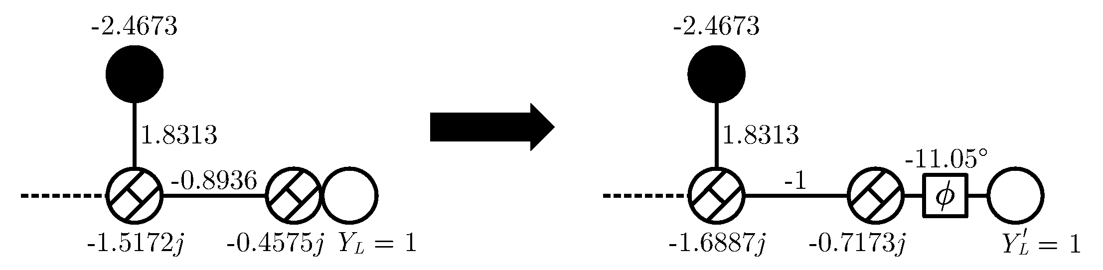
6. Experimental Validation

To validate the proposed methodology, a N = 5 order filter has been synthesized using the procedure in [6], symmetric polynomial definition, $RL=20$ dB, and allocation of the transmission zeros in the lowpass domain ${\Omega }_k=\{1.7342,-1.8170,1.2350,$$-2.2460,2.4673\}$ rad/s. The extracted elements of the lowpass prototype are shown in

Table 8. Lowpass elements of the synthesized 5th-order ladder filter before and after $J_{N+1}$ redistribution.

Parameters	${\mathit{B}}_{\mathit{kb}}$	${\mathit{b}}_{\mathit{kb}}$	${\mathit{J}}_{\mathit{rkb}}$	${\mathit{B}}_{\mathit{ka}}$	${\mathit{b}}_{\mathit{ka}}$	${\mathit{J}}_{\mathit{rka}}$
Res. 1	−1.004	1.734	1.110	−1.004	1.734	1.110
Res. 2	2.686	−1.817	2.095	2.686	−1.817	2.095
Res. 3	−1.042	1.235	0.944	−1.042	1.235	0.944
Res. 4	3.624	−2.246	2.841	3.624	−2.246	2.841
Res. 5	−1.517	2.467	1.831	−1.688	2.467	1.831
Source	−0.773			−0.773
Load	−0.457			−0.713

. The elements with subscript b correspond to those obtained directly from the synthesis procedure. In this case, the last inverter $J_{N+1}=-0.8936$, from the phase point of view, Figure 13 shows that ${\theta }_{11}={\theta }_{22}$ as expected since symmetric polynomials have been used.

The dangling resonator can only be serialized if the side inverters are equal with the opposite sign. As was previously discussed, a possible solution consists of applying a redistribution of the values of the last three elements of the network, the last two FIRs and the admittance inverter coupling them, to turn the last admittance inverter unitary. This is seen in the elements with subscript a in Table 8, where the FIR $B_{ka}$ for resonator 5 and the load elements have been modified. In this case, as expected, the last inverter $J_{N+1}=-1$ so the serialization is possible; however, a phase shift of $-{9.7}^{\circ }$ in the main-line is required for the exact and complete synthesis. The lack of such phase shifter entails that ${\theta }_{11}\ne {\theta }_{22}$ leading to a phase difference ${\theta }_{22}$−${\theta }_{11}$ = −22.1${}^{\circ }$.

For the sake of clarity, in Figure 14, the nodal representation of the directly synthesized network is compared with the network once the element transformation is carried out to achieve the $J_{N+1}=-1$. Therefore, the presence of the phase shifter in the main-line path is mandatory to have a perfect equivalence between both networks.

To have an exact and complete synthesis of the filter, the proposed phase correction method has been applied with $\psi =-{27.7}^{\circ }$ and $\varphi =-{89.3}^{\circ }$. In this case, the resulting last inverter $J_{N+1}$ = −1 as expected. The transformation to the bandpass domain results in the very well-known Butterworth-Van Dyke equivalent circuit [6] as shown in Figure 15a, where the value for the elements are summarized in

Table 9. Bandpass elements of the 5th-order ladder filter with phase correction terms $\varphi =-{89.3}^{\circ }$, $\psi =-{27.7}^{\circ }$.

Parameters	${\mathit{L}}_{\mathit{a}}$ (nH)	${\mathit{C}}_{\mathit{a}}$ (pF)	${\mathit{C}}_0$ (pF)
Res. 1	53.18	7.35	13.28
Res. 2	81.14	8.90	15.13
Res. 3	135.24	2.68	11.03
Res. 4	48.83	16.59	18.33
Res. 5	41.63	14.86	6.65
Source	73.3 nH
Load	4.74 pF

. The frequency transformation has been done considering $f_0=245$ MHz and BW $=100$ MHz.

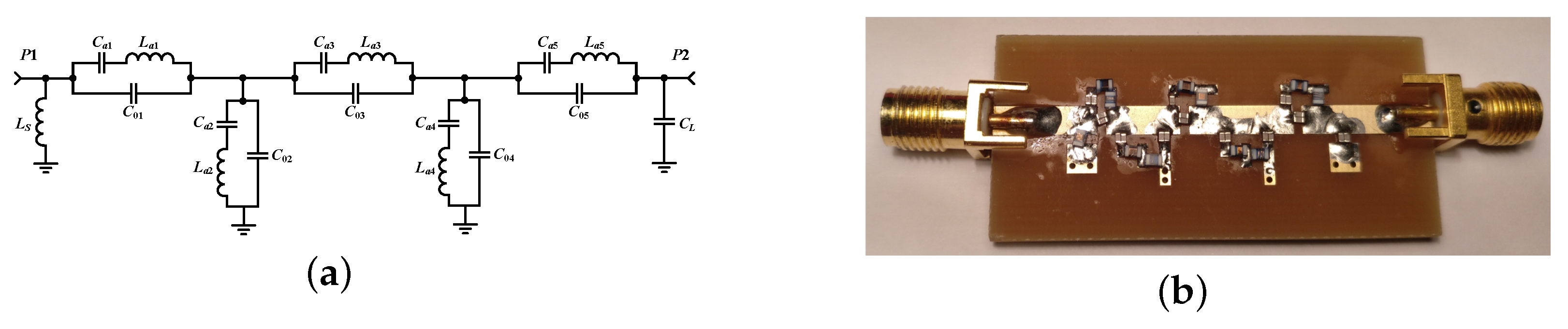
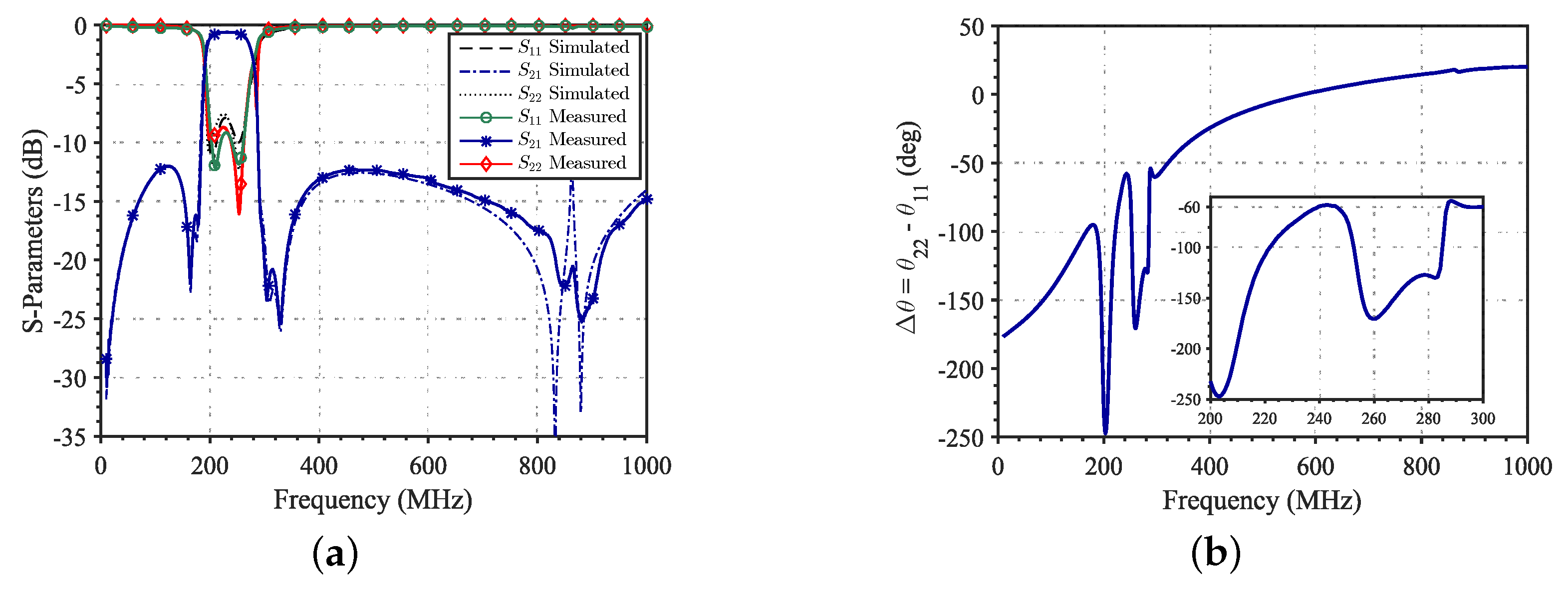
As a proof of concept and for rapid prototyping, the filter was made in FR4 with ENIG surface finish. The resonators were implemented with Wirewound High-Q Chip Inductors and Multi-layer High-Q Capacitors from Johanson Technology. The estimated Q factor for inductors and capacitors are, respectively, $Q_L=45$ and $Q_C=800$. The measured transmission response, as well as the input/output reflection coefficient, are shown in Figure 16a. The insertion losses are $-0.6$ dB as expected from the EM simulation, taking into account the finite Q factor of the lumped components. The tolerances in the used commercial values of the components are also responsible for the detuning of the upper TZ closest to the bandpass, which at the same time results in a certain degradation of the RL and achieved BW.

On the other hand, Figure 16b shows the measured difference between the phase of the input and output reflection coefficient $\Delta \theta ={\theta }_{22}-{\theta }_{11}=-{58.73}^{\circ }$. The response is in a very good agreement with the specifications of the filter where the theoretical difference is $\varphi -\psi ={\theta }_{11}-{\theta }_{22}=-{61.6}^{\circ }$. It has to be highlighted that in this case, unlike the method based on the redistribution of the network, no phase shifters are required for the serialization of resonators.

Figure 16. (a) Measured and simulated filter transmission response, and input/output reflection coefficient. (b) Difference between input and output measured reflection coefficient phase $\Delta \theta ={\theta }_{22}-{\theta }_{11}$. The simulation was carried out with ANSYS^® Electronics Desktop 2021 R1. The manufactured filter was characterized with the network analyzer N5242B PNA-X.

Figure 16. (a) Measured and simulated filter transmission response, and input/output reflection coefficient. (b) Difference between input and output measured reflection coefficient phase $\Delta \theta ={\theta }_{22}-{\theta }_{11}$. The simulation was carried out with ANSYS^® Electronics Desktop 2021 R1. The manufactured filter was characterized with the network analyzer N5242B PNA-X.

7. Conclusions

The benefits of the work presented in this paper is twofold. First, it is an observation of a phenomenon and a full description of it have been provided. When using the extracted-pole method with inline topologies, the use of symmetrical polynomials for non-symmetrical transmission zeros distribution translates the asymmetry not only into the resonance frequencies but also into the main-line admittance inverters strength. This situation introduces some difficulties to serialize resonators in the case of ladder topologies. However, they arise mainly when the ladder participates in a parallel-connected network. In this paper, the necessity of asymmetric polynomials for asymmetric networks to overcome phase offsets when using symmetric Chebyshev polynomials was presented and validated. To equalize all the admittance inverters in the main-line path to the same value, a novel method was found enabling the extraction procedure by correcting the Chebyshev polynomials phase for inline networks. It was observed that all suitable pair of phase values can be computed with a phase map. Additionally, we analyzed every aspect of it, and linked to an already existing solution by proving that it is merely a particular case of a more complex situation. Second, an algorithm was described to create a systematic and low-computing cost solution to make a better use of such observation for the filter designer benefit. Finally, a ladder-type filter was fabricated and measured to validate the proposed methodology.

References

1. Amari, S.; Macchiarella, G. Synthesis of inline filters with arbitrarily placed attenuation poles by using non-resonating nodes. IEEE Trans. Microw. Theory Technol. 2005, 53, 3075–3081. [Google Scholar] [CrossRef]
2. Macchiarella, G. Generalized Coupling Coefficient for Filters With Nonresonant Nodes. IEEE Microw. Wirel. Compon. Lett. 2008, 18, 773–775. [Google Scholar] [CrossRef]
3. Glubokov, O.; Budimir, D. Extraction of Generalized Coupling Coefficients for Inline Extracted Pole Filters With Nonresonating Nodes. IEEE Trans. Microw. Theory Technol. 2011, 59, 3023–3029. [Google Scholar] [CrossRef]
4. Tamiazzo, S.; Macchiarella, G. Synthesis of Cross-Coupled Prototype Filters Including Resonant and Non-Resonant Nodes. IEEE Trans. Microw. Theory Technol. 2015, 63, 3408–3415. [Google Scholar] [CrossRef]
5. Cameron, R.J. Advanced Filter Synthesis. IEEE Microw. Mag. 2011, 12, 42–61. [Google Scholar] [CrossRef]
6. Giménez, A.; Verdú, J.; Sánchez, P.D.P. General Synthesis Methodology for the Design of Acoustic Wave Ladder Filters and Duplexers. IEEE Access 2018, 6, 47969–47979. [Google Scholar] [CrossRef]
7. Verdú, J.; Evdokimova, I.; de Paco, P.; Bauer, T.; Wagner, K. Systematic synthesis methodology for the design of acoustic wave stand-alone ladder filters, duplexers and multiplexers. In Proceedings of the IEEE International Ultrasonics Symposium (IUS), Washington, DC, USA, 6–9 September 2017; p. 1. [Google Scholar]
8. Giménez, A.; de Paco, P. Involving source-load leakage effects to improve isolation in ladder acoustic wave filters. In Proceedings of the IEEE MTT-S International Microwave Symposium (IMS), San Francisco, CA, USA, 22–27 May 2016; pp. 1–4. [Google Scholar]
9. Triano, A.; Verdú, J.; de Paco, P.; Bauer, T.; Wagner, K. Relation between electromagnetic coupling effects and network synthesis for AW ladder type filters. In Proceedings of the IEEE International Ultrasonics Symposium (IUS), Washington, DC, USA, 6–9 September 2017; pp. 1–4. [Google Scholar]
10. Triano, A.; Verdú, J.; de Paco Sánchez, P. A General Synthesis Technique of Mixed-Topology Including Parallel-Connected Structures for Fully Canonical Ladder-Type Acoustic Filters. IEEE Trans. Microw. Theory Technol. 2019, 67, 5061–5068. [Google Scholar] [CrossRef]
11. Triano, A.; Silveira, P.; Verdú, J.; de Paco, P. Phase Correction of Asymmetrical Chebyshev Polynomials for Extracted-Pole Fully Canonical Filters. In Proceedings of the IEEE MTT-S International Microwave Symposium (IMS 2019), Boston, MA, USA, 2–7 June 2019. [Google Scholar]
12. Cameron, R.; Mansour, C.K. Microwave Filters for Communications Systems: Fundamentals, Design, and Applications; Wiley: Hoboken, NJ, USA, 2007. [Google Scholar]
13. Tsutsumi, J.; Matsumoto, K. Super-Isolation Duplexer Aiming for Removing Rx Inter-stage Filter in W-CDMA Handsets. In Proceedings of the 38th European Microwave Conference, Amsterdam, The Netherlands, 28–30 October 2008; pp. 1066–1069. [Google Scholar]
14. Rhodes, J.D.; Cameron, R.J. General Extracted Pole Synthesis Technique with Applications to Low-Loss TE011 Mode. Filters 1980, 28, 1018–1028. [Google Scholar]
15. Cameron, R.J. Fast generation of Chebyshev filter prototypes with asymmetrically-prescribed transmission zeros. ESA J. 1982, 6, 83–95. [Google Scholar]
16. Cameron, R.J. General coupling matrix synthesis methods for Chebyshev filtering functions. IEEE Trans. Microw. Theory Technol. 1999, 47, 433–442. [Google Scholar] [CrossRef]
17. He, Y.; Wang, G.; Sun, L. Direct Matrix Synthesis Approach for Narrowband Mixed Topology Filters. IEEE Microw. Wirel. Compon. Lett. 2016, 26, 301–303. [Google Scholar] [CrossRef]
18. Fanchi, J. Math Refresher for Scientists and Engineers; Wiley: Hoboken, NJ, USA, 2006. [Google Scholar]
19. Lundsgaard, H. Shadows of the Circle: Conic Sections, Optimal Figures and Non-Euclidean Geometry; World Scientific Publishing Company: Singapore, 1998. [Google Scholar]
Figure 1. Lowpass nodal scheme of an inline prototype filter with N transmission zeros.
Electronics 10 03058 g001
Figure 2. S-parameters of the extracted filter using TZs distributions Ω A k and Ω B k .
Electronics 10 03058 g002
Figure 3. Nodal diagram of the last three elements of the network before (left) and after (right) the admittance redistribution. The grey elements are actually part of the network but they are irrelevant in this scenario.
Electronics 10 03058 g003
Figure 5. (a) Horizontal hyperbola and (b) vertical hyperbola representation. The black trace represents those combinations of ϕ , ψ that yields | J N + 1 | = 1 . For illustration purpose all | J N + 1 | values that fit in 1 ± 0.001 have been plotted. The red traces corresponds to the asymptotes. The point ( ψ 0 , ϕ 0 ) is the origin and ( ψ 0 , ϕ 0 ) the origin of another hyperbola with a 180 shift in both directions.
Electronics 10 03058 g005
Figure 7. (a) Horizontal hyperbola of the filter with Ω B k TZs and (b) vertical hyperbola of the filter with Ω C k TZs. The black trace are those combinations of ϕ , ψ that yields | J N + 1 | = 1 ± 0.001 . The red line across the ϕ axis is at ψ = 0 .
Electronics 10 03058 g007
Figure 8. (a) S-parameters of the network with Ω E k TZs and (b) the phase map of the ellipse with a sweep between ± 180 .
Electronics 10 03058 g008
Figure 9. Comparison between the phase sweep in ϕ for the filter with Ω t z 1 TZs and the parabolic estimation model.
Electronics 10 03058 g009
Figure 13. Input and output reflection coefficient θ 11 and θ 22 .
Electronics 10 03058 g013
Figure 14. Network with the direct synthesis of the elements resulting in J N + 1 1 (left), and once the network transformation is done to achieve J N + 1 = 1 (right).
Electronics 10 03058 g014
Figure 15. (a) Equivalent electric circuit using the Butterworth-Van Dyke model for the designed filter, and (b) the fabricated prototype using lumped elements.
Electronics 10 03058 g015