1. Introduction
LDPC codes can approach Shannon’s capacity with moderate decoding complexity at low SNRs [
1,
2]. However, maximizing the full potential of the LDPC codes requires accurate timing recoveries in the baseband process of the receivers. Traditionally, timing recovery is performed independently from channel decoding. However, the metrics generated from channel decoding can generate more reliable information in iterative timing recovery [
3]. The generated information can be applied to assist timing recovery in order to obtain accurate synchronization at very low SNRs. Traditional methods are usually ineffective at low SNRs. Iterative timing recovery uses the metrics from the codewords output of the channel decoding process [
3]. A method with LDPC decoding hard decision metrics (i.e., code constraint feedback) to obtain good timing recovery has been proposed in [
4]. However, it suffered from insufficient hard metrics, or unreliable satisfaction percentages of decoded codewords for the parity check equation for just few iterations [
4,
5]. Studies also suggested the use of timing recovery based on soft LDPC metrics with complex optimization calculations [
6]. Other expectation maximization (EM)-based timing recovery methods for turbo or LDPC coding have also been suggested [
7,
8]. The EM-based timing recovery method is implemented between the detection and estimation processes, where the expectation of symbols is calculated by a maximum a posteriori (MAP) decoder. Afterwards, the cost function is maximized to acquire excellent symbol timings. For instance, the EM algorithm has been applied in solving the time and frequency synchronisation in a multiple-input multiple-output (MIMO) orthogonal frequency-division multiplexing (OFDM) system [
9]. However, the function has highly complex EM steps. Several turbo decoding-aided timing recovery, with timing recoveries incorporated into iterative decoding, have been proposed for blind turbo detection of synchronization parameters [
10]. Here, a turbo component decoder is applied in the synchronization parameters to perform blind joint synchronization detection and decoding with decoded metrics. In [
11], synchronisation is incorporated into Turbo decoding as the blind detection of synchronisation parameters. It uses a turbo component decoder to perform blind synchronisation detection and Turbo decoding by the decoding metrics. In [
12], a new objective function is maximised to exploit the output turbo decoder’s soft decision to improve synchronisation iteratively. Thus, it is suited for short bursts of data transmissions at low SNRs. In [
13], a Turbo soft metric based cost function is maximized to exploit the turbo soft decision and iteratively improve the synchronization. Thus, turbo-decoding metrics are calculated for obtaining good timing recoveries at low SNRs. However, turbo code-based methods are highly difficult due to complex turbo decoding. Because large sampling frequency offset can cause huge synchronization searching calculation and delay, a sampling frequency synchronization method to eliminate initial sampling frequency offset can also help reduce the overall synchronization time for the coarse symbol timing recovery [
14]. So the communication receives require the iterative timing recovery to acquire rather large timing frequency and phase offsets for good timing synchronizations. In addition, the iterative timing recovery can be performed by the means of MAP criterion as the iterative carrier synchronization but with much high complexity [
15]. Therefore, an iterative timing recovery with high precision and low complexity is needed for using in space communications which usually work at low SNRs.
In this study, we mainly propose a new iterative timing recovery scheme by using the LDPC decoding metrics to correct timing errors for better timing precision and lower complexity. The timing recovery mechanism are modelled as an optimization problem of maximizing the sum of the squares of selected LDPC decoding metrics for precise estimation of timing offsets. Then, a theoretical verification is demonstrated analytically with closed expressions of the transition trend of the probability mean of the soft decoding metrics by the Gaussian approximation. In addition, an efficient numerical technique of approximate stochastic gradient descent is employed to solve the above optimization problem of excellent timing recovery with rational computations. Finally, a traditional M&M timing recovery algorithm [
16] is adopted to rectify residual timing errors by using the LDPC code words as the anticipated data needed in timing track loops. Thus, it also saves some more bandwidth resources brought by trained data in traditional timing recovery schemes, which endows it more pragmatic in spectrum efficient satellite communications.
The remainder of the paper is organized as follows. In
Section 2, the concept of the timing error model is introduced.
Section 3 gives the principle of the suggested iterative timing recovery with soft LDPC decoding metrics. In this section, Gaussian approximation method is employed to explain the evolution trend of the soft metrics, which are influenced by the timing errors. The proposed iterative timing recovery scheme, accompanied by the traditional M&M timing track algorithm, is stated in
Section 4 for the final timing synchronization scheme. In
Section 5, the numerical simulations are given to manifest the good performance of the proposed scheme. In this section, we also analyze the possible reasons for the good performance of our proposed scheme and evaluate the computation complexity. Finally, the conclusion is drawn in
Section 6.
2. Timing Error System Model
Each transmitted symbol in a binary phase shift keying (BPSK) system is composed of
N point impulse responses
from a square root raised cosine (SRRC) pulse shaping filter with
L times sampling rate, where
T is the symbol interval. The signals are shaped as sequences (
) in the above filter, where
is the
i-th modulated symbol and
is the sample symbol interpolated with (
) zeros between every two adjacent
to fit the sampling rate.
is the timing offset to influence the
m-th sample. Thus, the signal
for transmission is given by
A received sequence with
L-times up-sampling rate without timing offsets is expressed as
where
is the received signal,
is the additional white Gaussian noise (AWGN) from the channel, and
is the sampling interval. The assumed time reference for the
m-th sample at the receiver when timing errors occur differs from the corresponding sample at the transmitter with timing offset
. The
m-th sampled signal after
L times down-sampling is presented as
Finally,
is obtained by replacing
with the above expression. The resulting equation is presented as follows.
Constant timing frequency offset and random walk [
4] can be combined in our model, because proper timing error models exist as constant timing phase offsets. The combined equation is presented as
where the initial time instance is offset by constant timing phase offset
D, the timing error is disturbed by a zero mean Gaussian random variable (random walk) with variance
denoted by
, and the constant timing frequency offset
is measured in parts per million (
). They should be estimated and compensated precisely for high transmission effect.
3. Influence of Timing Errors on LDPC Decoding
The received baseband signals are raised-cosine pulses from the combination of SRRC pulse-shaped filters located at the transmitters and receivers along with the AWGNs. In [
6], the sampling positions approached the sampled points from LDPC decoding and corresponding analyses, which led to the increased absolute value of all LDPC decoding metrics, i.e., log-likelihood ratios (
). A similar effect of the sum of all
squares under these timing errors also manifested. This phenomenon is explained below.
Given no noise, a received signal with perfect timing is properly sampled at the center of the symmetry raised cosine signal waveform and it has the most effective amplitude. However, under the overall timing offset as presented in Equation (
5), the sampled signal deviates from the optimal center of the waveform with less effective amplitude and it is further deteriorate by the inter-symbol interference (ISI) by adjacent signals. At low SNR, the influence of the ISI can also be approximately modeled as the AWGN [
10]. Therefore, the comprehensive effect of the symbol timing error causes a decreased effective SNR for the coded BPSK modulation system. The equivalent noise variance is the sum of the original noise variance and the new generated equivalent noise variance caused by the ISI. With SNR analyses in [
8], more deviations from optimal sampled points cause lower SNRs for the received signals, leading to a decrease of initial messages (i.e.,
) in LDPC decoding. The final output messages in the decoding are dependent on the square of the initial messages, because the messages in the iterations are mainly dependent on the square of previous messages. In addition, the sum of the square of each message increases the deviation effect. Thus, when timing offsets are introduced to reduce the effective SNRs, the amplitude of the initial messages decreases; in turn, this reduces the
and decreases the sum of the square of all decoding messages. This process can be analyzed with density evolution and Gaussian approximation [
17,
18].
Firstly, we give a typical instance of the schematic diagram of the LDPC decoding by the iterative belief propagation (BP) [
1,
2] algorithm as shown in
Figure 1.
From
Figure 1, at an AWGN channel with zero mean and variance
, the logarithm version of the LDPC decoding can be expressed as below.
(1) Initialization
The initial soft metrics of LDPC decoding, i.e.,
, are expresses as
where
is the logarithm likelihood ratio (
) function and
is the initial
of the codeword
.
and
are the
i-th decided and received signals respectively.
and
are the exchanged messages between the variable node
j and the check node
i.
(2) Decoding procedure
- -
(2.1) Update the variable nodes and perform the final decoding judgment
The decoding metrics updated in the variable nodes and final decoding judgment can be expressed as
where the set of the
i-th check node connected to the
j-th variable node is expressed as
and
is the element of the check matrix
with index (
). The symbol “
” behind a set means the set with removal of the element “
j”.
is the LDPC soft decision metrics of the
i-th variable node of the codeword
.
N is the code length.
is the codeword vector and the estimate of this vector is
. In this step, if
,
is the decoding result. If
is the result or the iteration exceeds the maximum times, the iteration is finished. Otherwise, go to next step (2.2).
- -
(2.2) Update the check nodes and then go to step (2.1)
The decoding metrics updated in the check nodes can be represented as
and then go to step (2.1) for subsequent processing.
In Equation (
11), the set of the
j-th variable node connected to the
i-th check node is
.
Then, the messages from the
j-th variable node and the
i-th check node in LDPC decoding (given as
and
, respectively) are symmetrical with
, where
and
m are the variance and mean value of the messages, respectively [
17]. The mean value of all messages for variables and check nodes (
and
) are updated in the iterations. The mean values represent the probability distribution of the messages. The mean value of the messages
from the variable nodes to the check nodes in
k-th iterations is presented as
where
is the mean value of messages from all check nodes and variable nodes
v after
iterations,
is the mean value of the initial message
, and
is the variable node degree. The indexes of
and
can be omitted for simplification, because they are independent and identically distributed (
i.i.d.). Moreover,
is assigned to a zero mean value, because initial messages from all check nodes are zero. The updated messages coming from check nodes to variable nodes are presented similar to [
6] as
where the indexes
and
are omitted because they are
i.i.d., and
is the check node degree.
is presented as
where “
R” represents that the integral interval falls in the entire field of real number.
Moreover, a new function
is defined in [
17] as
Equation (
15) is continuous and monotonically decreases on
with (
,
). The mean value update of all messages from the check nodes to the variable nodes is given by
where
is zero, which is the initial value of
[
18].
The output messages from the variable nodes
after
k iterations are represented as
From Equation (
17),
is mainly decided by initial message
and message
after
k iterations. In addition,
can be recursively calculated by Equation (
16) and
with an initial value of
. Thus,
relies on the mean value of initial message
. The properties of
indicate that a larger
leads to similarly larger values of
and
in Equations (
16) and (
17), respectively; thus,
is mainly decided by
. In addition, a larger
leads to a larger
and sum of all message squares. It can be explained as follows.
For the same LDPC codeword, the main code parameters, i.e., the degree distribution, are the same. So the variable node degree
and check node degree
are equal for a specific node message processing under different channel state information, or the initial LLR represented in Equation (
6). From Equation (
15), the function
is continuous and monotonically decrease on its definition domain
with (
,
). Then, due to the relationship that a function and its inverse function is just mirror symmetrical about the function
, the inversion function
is also decrease on
with (
,
). So the first recursive iteration of the messages from the check nodes to the variable nodes in Equation (
16) is given as
where
is the initial message and it is got from Equation (
6). Obviously, due to the monotonically decrease property of
and
, larger
causes the larger
. For the second recursive iterations, Equation (
16) is expressed as
From Equation (
19), other parameters being the same, the larger initial message
along with the corresponding larger previous generated message
leads to a much larger
than that generated from a smaller initial message. The rest can be done in the same manner and in the higher order of recursive iterations, larger initial message
surely causes larger solution result
after
k recursive iterations.
Therefore, the conclusion is true for an LDPC-coded system with an all-0-bit input. A symmetry condition (
) is used to preserve the above conclusion for all messages, because initial negative messages can be processed for positive ones as follows [
18]. First, the channel symmetries are given by
The sign factor of the check node message map
is given by:
where
belongs to
sequence.
The most important sign inversion invariance property of the variable node message map
is expressed as:
The final output message
is dependent on the square of initial messages based on Equations (
12)–(
22). The non-0-input messages, which correspond to the minus data in the iterations, are also dependent on the square of message
based on the symmetry properties shown in Equations (
20)–(
22). Thus, larger squares of initial legal LDPC codeword messages lead to larger squares of final output messages. The sum of the above equations amplifies this effect. Initial message amplitudes (i.e.,
) decrease when timing offsets are introduced to reduce the effectiveness of SNR. The decrease reduces the cost function, i.e., the sum of all the square of the
Thus, a timing offset estimate (including timing phase and frequency offsets) is obtained by searching possible ranges in obtaining the maximum cost function. Moreover, random walk has limited destructive effects, because it is limited by oscillation quality. Therefore, optimal timing offsets are estimated and corrected by maximizing the sum of all the square of the
.
4. Proposed Iterative Timing Recovery
The
i-th message, (i.e.,
) in LDPC decoding [
2] is presented as
where
is the received signal vector with element
,
is the variance of channel noise,
is the decision of the
i-th element of
,
or
is the posterior probability of the decision of the received signal
, and
is is the extrinsic information brought by other variable nodes with relation to parity check constraint.
is updated for each LDPC decoding iteration from the parity check nodes. Correct
are crucial in ensuring proper LDPC decoding. Based on the analyses and conclusions presented in
Section 3, an efficient timing recovery can be developed as follows. First, an object function
related to the timing phase and frequency offsets,
and
(measured in
), is defined as
where
is
, and
K is the LDPC codeword length. Thus, the optimal (
) can be iteratively searched and updated by solving the optimization function given by
To illustrate the objective function
, a curve of it with respect to
after 3 LDPC iterations is calculated and shown in
Figure 2, where the LDPC code (1944, 972) in Draft IEEE 802.11n [
19] is selected at
/
of 0.5 dB. Based on the above numeric simulations, the object function
in Equation (
25) is symmetrical and approximately convex to its variable, i.e.,
. It indicates that the function
has a maximum value located at the position without any timing offset. Other cases are the same under different LDPC codes and
/
, where one global optimum value and some local ones are featured in the plots. Therefore, this being the case, the optimal estimation of
can be obtained by maximising the function
.
Thus, gradient descent algorithm (steepest descent) can be applied in solving Equation (
26) similar to [
13]. Afterwards, a two-dimensional gradient descent algorithm is carried out to iteratively search and update
for Equation (
26). An approximate gradient descent algorithm is used to implement the iterative timing recovery, because the object function
is discontinuous without direct analytic expressions. The iterative timing recovery process is discussed below.
Firstly,
in Equation (
25) is considered constant to
.
and
are set to zero for the 1st iteration (i.e., no message from the check nodes to the variable nodes) and hide in the change of
in other iterations of the subsequent derivations. Thus,
can be omitted in approximate derivations of
to
. The omission is calculated as
The received signal
, or mainly the variable
, is affected by the timing offset parameters
based on Equations (
23) and (
24). So the approximate derivation of
to
can be represented as
By similar techniques in [
13], given normalized parameters, the received signal
can be approximately modeled as follows:
where the amplitudes of the transmitted signals are normalized as “1”,
is the channel noise at that time instance, and “sgn” is the sign function in mathematics. Here, the approximate transition trend of
to
is used to incorporate a more accurate value into positive constant
and
, which can be determined in simulations. Equations (
29) and (
30) is then approximately calculated as
Equations (
32) and (
33) can be further simplified by uniting all fixed variables or constants into the negative value
and
, respectively, as
Thus, the calculation complexity can be reduced by Equations (
34) and (
35), because we use the adaptive parameter update algorithm, which just needs the approximate trend of the gradient rather than the more accurate numerical results. So the adaptive timing parameter correction along with the iterative LDPC decoding jointly contribute the good features of both good performance and low complexity.
Finally, according to the principles of the adaptive algorithms,
can be estimated and updated with the following Equations (
36) and (
37) as
where
and
are step parameters for iteratively updating
, respectively,
in Equation (
31) decodes LDPC codes, and the superscript
demotes the
(n)-th iteration. The partial derivation function
and
are computed in Equations (
34) and (
35). The initial parameter pair
can be set as the zero vector (0, 0). The other constants can be verified in the simulations.
In addition, a conventional first-order PLL-based structure with a decision-directed Mueller–Müller timing error detector (M&M TED) [
6] can also be used as a supplement like [
4] to implement the iterative timing tracking. At each iteration, the M&M TED is executed by provided with more accurate symbols decoded by the LDPC decoder and the re-sampled received signals, which are compensated with the optimal estimate of timing phase and frequency offset by our proposed algorithm. Finally, according to the above analyses, the whole timing recovery is designed in
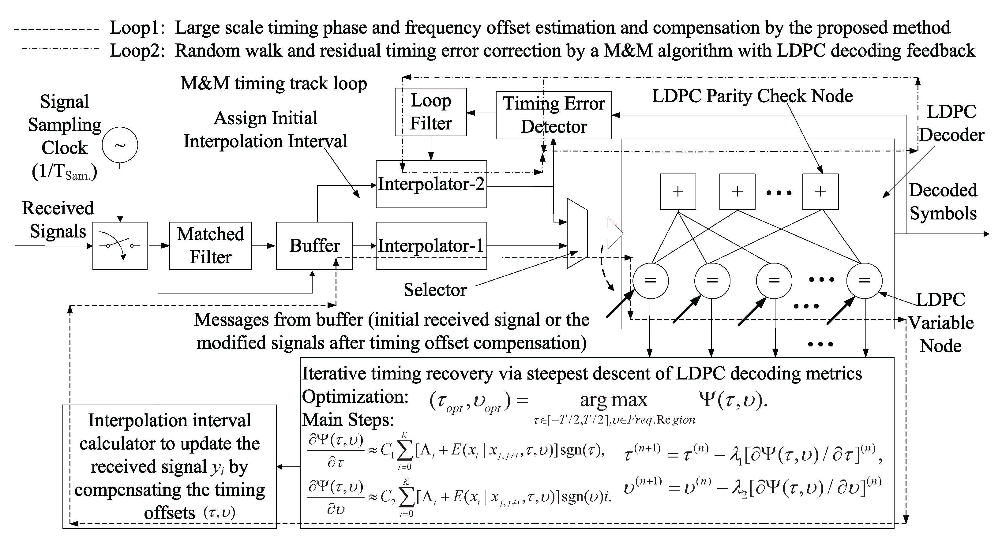
Figure 3.
In the whole timing recovery system shown in
Figure 3, there are two loops to execute the timing recovery, i.e., Loop1 and Loop2. The Loop1 is performed at first by our proposed iterative timing recovery via steepest descent of LDPC decoding metrics to obtain large scale timing phase and frequency offset estimations, which are used to compensate the error of the received signal
by Equation (
31) stored in the buffer in
Figure 3. The main steps of the procedure are calculated by Equations (
34)–(
37) to obtain the final optimized goal denoted in Equation (
26). So this loop mainly performs the timing capture, especially at low SNRs. After Loop1, the selector switches the working mode to Loop2. Then, random walk and residual timing errors are corrected by a M&M algorithm with the reference LDPC decoding feedback, which works as the timing track.
According to the above iterative timing recovery scheme, the computational complexity can be analyzed as follows. Here, we just calculate the additional computations other than the compulsory LDPC decoding. It is assumed that
L iterations of timing offset estimation and compensation in the length-
K LDPC code are required for the satisfied symbol timing recovery. From Equations (
34) and (
35), there are
K additions in the top equation and
K additions and
K multiplications in the bottom equation, which sum up as 2
K additions and
K multiplications. The coefficients of
and
in Equations (
34) and (
35) are empirical parameters and they can be incorporated into the step size of
and
in Equations (
36) and (
37). So the calculation of them can be neglected. Then, there are two multiplications and two subtractions (equal to additions in computational complexity) in the update of timing offset estimates in Equations (
36) and (
37). The step size parameters are decided by the practical occasions, which can be neglected, when compared with the above calculation. Moreover, there are three multiplications and three additions in the update of
in Equation (
31), plus 1 division (equal to multiplication) in the calculation of
, i.e.,
, in Equation (
6). Therefore, the total computational complexity, except from the necessary LDPC decoding, are approximate
additions and (
K + 6)
L multiplications. By later simulations, since the required iterations of the timing recovery are limited, i.e.,
, the total computational complexity is acceptable in practice.
5. Simulation Results and Analyses
To verify the effectiveness of the proposed scheme, numerical simulations of a LDPC coded BPSK system in an AWGN channel are carried out in this section. The LDPC code (1944, 972) [
19] is adopted in the simulations with a maximum of 20 decoding iterations. Generally, the performance is often weighed by bit-error-rate (BER). So Monte Carlo simulations of LDPC decoding will run until either a specified number (e.g., 10 in high SNR and 50 in low SNR) of error frames occur or a total 1 million trials have been run. We choose the above simulation parameters of iteration stop judgment for LDPC decoding by compromising the result reliability and calculation efficiency and also the more practical experiments in some powerful work stations. The SRRC shaped and matched filters both have a roll-off factor of 0.3 and 13 taps. Several timing offset estimation iterations are used. The timing phase and frequency offsets are set over ±0.5 T (e.g.,
T and
T is the sampling period) and ±500 ppm (e.g., 300 ppm). The parameter
of the random walk is 0.5%, which is similar to that used in [
5]. The step size parameters
and
in Equations (
36) and (
37) are chosen as 0.2 and 0.5, respectively. Finally, the parameter analyses and the BER performances by the proposed iterative timing recovery are simulated and shown as follows.
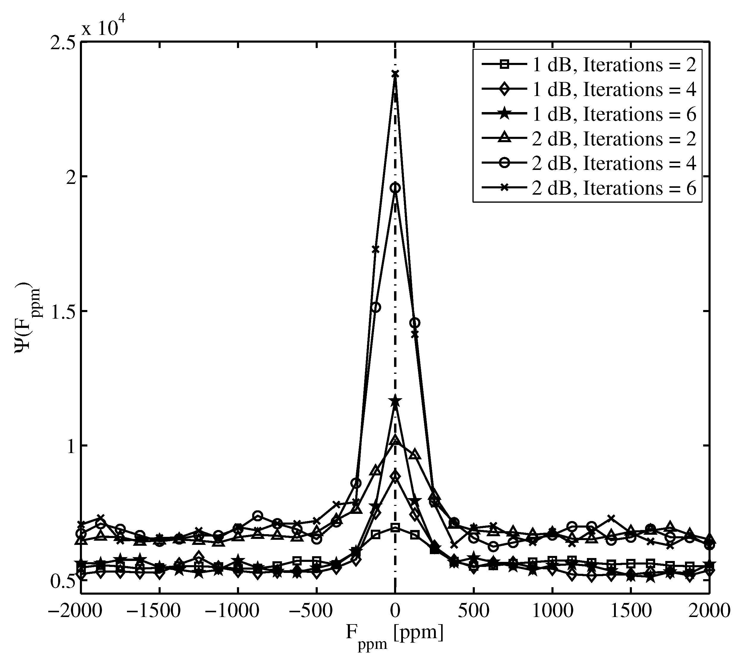
The partial curves of
to
, and the
to
and
to
, with two, four, and six iterations at
/
of 1.5 dB are shown in
Figure 4 and
Figure 5, respectively. The timing phase offsets within
T occur near the optimal position (
Figure 4).The closeness to the optimal position is mainly due to the property of the raised cosine waveform by the SRRC-shaped and matched filters, where
within
T slightly reduces the effective amplitude of the received signals. Furthermore, the influence of
on
changes dramatically (
Figure 5). The largest frequency error discrimination occurs within 20 of the optimal point. Thus, approximately 6 iterations are enough for the timing recovery to distinguish the ideal sampling point. Further from this simulation, the effective search ranges for the timing phase and frequency offsets are chosen as
0.5 T, 0.5 T) and (−500 ppm, 500 ppm). This may be the deficiency of the proposed timing recovery, where traditional timing recovery should be performed at first to guarantee the residual timing offsets fall into the range of this requirement. However, the proposed timing recovery can obtain much better estimation precision.
Here, we define the normalized mean square error (NMSE) simulations for
as
and
in Equations (
38) and (
39) as
where
are real timing phases and frequency offsets, whereas
are their estimates. Moreover, the estimated timing error parameter pair
involves an average of 50 times calculation. Meanwhile, the true timing error parameter pair
for test cannot be the vector with any element zero to make sense of Equations (
38) and (
39) avoiding from divided by zero. Then, the
and the
with four, six, and eight iterations at different SNRs are simulated and shown in
Figure 6 as follows.
The
in
Figure 6 is smaller than
, because the influence of
on object function
exerts more control than
(
Figure 6).
Therefore, a total of six iterations are enough for timing recovery (
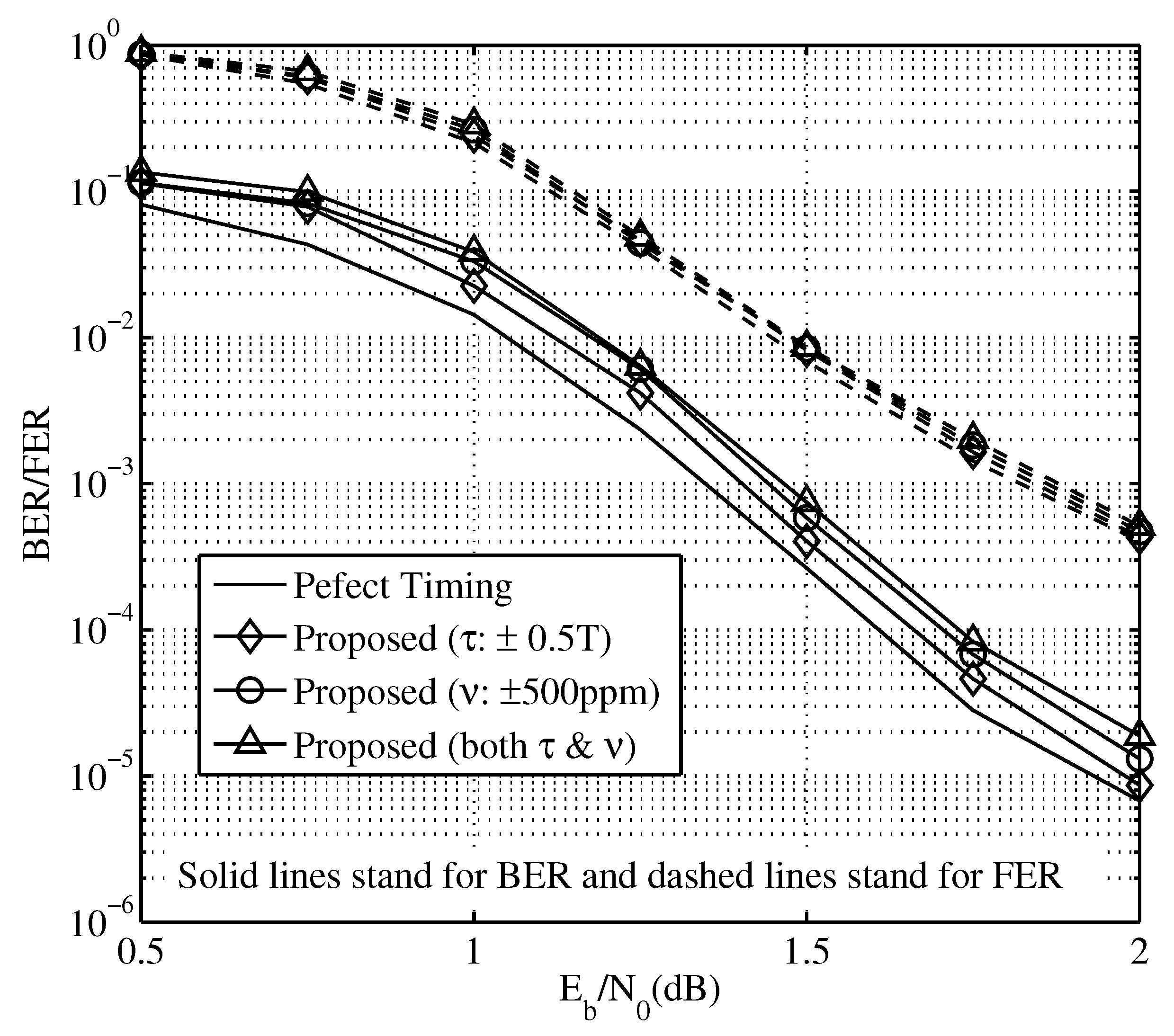
Figure 6). In our scheme, 6 timing recovery iterations are simulated and compared with the ideal code performance. The bit or frame error ratio (BER/FER) of the scheme with the above parameters is shown in
Figure 7.
The performance of the LDPC coded system, which suffered from large timing errors, is within 0.1 dB of the ideal code performance (
Figure 7). The LDPC coded system performs well at low SNRs (i.e., below 1 dB) without any pilot symbols. The cost is trivial, because the complexity linearly grows with the LDPC code length. In addition, incremental operations are limited.
Finally, our algorithm is more stable than the algorithm in [
4] because our algorithm employs soft decisions, whereas [
4] uses hard decisions as code constraint feedback. Hard decisions yield false judgments when even decoded bits are reversed falsely, which involves computing the same parity check equation. In comparison, no similar case of false judgment exists in our algorithm. Therefore, our scheme shows rational complexity and excellent performance similar to [
4]. However, our algorithm is more stable in timing recoveries especially at low SNRs.
The complexity increment for the timing recovery scheme can be analysed in the comparison between the original scheme with traditional timing recovery and LDPC decoding, and the proposed scheme with the iterative timing recovery, the residual timing recovery and LDPC decoding. The traditional scheme performs the timing recovery and LDPC decoding separately. It has one timing tracking calculation for each sample and several LDPC decoding iterations. However, under the same condition and LDPC decoding iterations, our scheme has the same LDPC decoding computations and timing tracking calculation, including some extra calculations of iterative timing recovery. By Equations (
34)–(
37), and given iteration number
, there are about
additions and
multiplications of additional computations in our scheme. Actually, with the gradual correction of timing errors by the proposed iterative timing scheme, the equivalent SNR is improved too. So the iteration number of LDPC decoding can be significantly reduced by sharp reduction of the decoding iterations. So it also magnificently cut down the computational complexity for the whole iterative system. However, it is difficult to illustrate this procedure analytically due to the nature of iterative process, which is closely related to the initial input signals and nonlinear iterative calculation. So the computational complexity cost of the proposed scheme is determined by initial input parameters and precision required in the joint decoding and demodulation. Thus, it can only be evaluated by numerical methods dependent on random input modulated signals.
In our former work [
6], it employs similar metrics from LDPC decoding to achieve timing synchronization at low signal-to-noise ratios. It obtains the accurate timing acquisition with a search window based Nelder-Mead simplex algorithm [
20] to maximize the sum of the absolute values of the metrics. It obtained a little performance gain (≤0.05 dB) than our new proposed algorithm. However, it may encounter the problems of local convergence of the optimization searching algorithm under limited iterations. It had to add some more additional decision module to judge and overcome the convergence problem. In our proposed method, it can achieve the same performance and overcome the deficiency of local convergence of the suggested optimization brought by the iterative BP decoding. It can be explained as follows. Due to the analyses of the influence of timing offsets on LDPC decoding, the effect of the timing error can be modeled as the decrease of SNR in the decoding procedure. The actual SNR can be the synthesis of the real AWGN noise and the equivalent AWGN noise caused by the inter symbol interference (ISI) due to the false symbol sampling. It can be improved via our proposed method in the several timing parameter updates in Equations (
36) and (
37). As long as the LDPC decoding is convergent within the range of decoding threshold, the proposed iterative timing recovery is surely to be globally convergent too, thus guarantee the effectiveness of the proposed timing recovery. In addition, it can also turn to the help of an additional Mueller–Müller algorithm [
16] for better symbol synchronization, where it plays a similar role of timing synchronization tracking. Furthermore, the proposed algorithm can be further simplified by accumulating the metrics from LDPC variable nodes with high degrees, which holds reliable metrics in the LDPC decoding. It has been verified by numerical simulations with the similar method, except that the calculation of Equation (
25) just includes the more reliable variable nodes of high degree. Because the results are exactly similar for the further simplified algorithm with reduced variable node calculation, we will not repeat the redundant result here for the purpose of saving space. In addition, the portion of the low degree variable nodes, that do not take part in the accumulation of Equation (
25), should be less than 20% via several simulations. Otherwise, there will be too many fluctuations to affect the approximately convex of the objective function
shown in
Figure 2, which greatly affect the effectiveness of the proposed iterative timing recovery. Suppose the portion of the high degree variable nodes to the whole code length is
p, the whole complexity can be further reduced to the
p of the proposed algorithm.
In our work, we mainly discuss the least complex BPSK modulation scheme. We mainly focus on the development of iterative timing recovery itself, so we just use it to illustrate our idea. Actually, long distances in satellite communications and the corresponding low signal-to-noise rate (SNR) transmission environments require power-efficient low-order modulation, such as BPSK, quadrature phase shift keying (QPSK) and some variations of it (e.g., offset quadrature phase shift keying (OQPSK),
-differential quadrature phase shift keying (
-DQPSK), etc.). Our scheme can be simply modified to satisfy these modulations, since the QPSK modulation series are actually the orthogonal implementation of two group of BPSK, and each branch of BPSK can adopt our proposed timing recovery scheme to accomplish the timing synchronization. The timing recovery scheme can be further improved with the well-known Costas loops for good implementation in practice. In these schemes, we obtain the metrics from the modulated signals in an orthogonal manner to feed the LDPC decoder, and the timing recovery parameters are iteratively calculated in LDPC decoding similar to those in our scheme. In addition, we also verify the roughly convex of the sum of the squares of selected LDPC decoding metrics with QPSK modulation similar as that shown in
Figure 2. The efficient approximate stochastic gradient descent algorithm is also feasible. The complexity growth is still acceptable since only two branch of BPSK synchronization loops are required in the QPSK related schemes other than one branch in our scheme. The complexity increment is rather trivial. For more complex modulations, such as the Mary-quadrature amplitude modulation (
M-QAM), Mary-phase shift keying (
M-PSK) and even the Mary-amplitude phase shift keying (
M-APSK) modulations, they can also be divided as the In-phase and Quadrature-phase mode of amplitude-shift-keying (ASK) modulations to properly implement the proposed timing recovery scheme. The complexities mainly lie in the metric extraction from the high-order modulations. They can be the further works in this aspect of research for low complex approach. Finally, due to the similar main mechanism of soft LDPC metric usage in timing recovery, we do not expand these contents more for purpose of concise manuscript. However, they can be simply derived and constructed for practical applications in satellite and wireless communications.


