A New Approach to Compensator Design Based on Multi-Loop Technique and Scalable Forward Model Complexity

Abstract

Using a compensator in the structure is one of the simplest ways to achieve efficient control of a non-linear process. Unfortunately, accessing the inverse process model is not a trivial issue. Except for some special cases, it is much easier to determine the forward process model than the inverse one. For this reason, it would be interesting to propose an alternative solution to the well-known feedforward control method. In this paper, a simple multi-loop concept will be introduced. The main idea is based on the natural (but limited) robustness offered by a single PID loop and the ability to scale up the complexity of the forward process model. The proposed structure multiplies a single PID loop including forward models with increasing complexity to calculate the resultant non-linear control value. This new approach produces a comparable performance to the feedforward method but does not require access to the inverse properties of the process. The idea was evaluated in terms of stability and robustness to parameter changes. In addition, a simulation study was carried out using two coupled non-linear processes, i.e., the position control of a robot manipulator with force interaction. The selection of this process was no casual choice. On the one hand, it is extremely complex; however, on the other hand, it provides the possibility to determine both the inverse and the forward dynamic model. This capability was helpful to perform an effective comparison of the proposed solution with the known feedforward structure.

1. Introduction

The fundamental problem in feedback control design is the ability of the control law to guarantee the stability and robustness of the whole system. Many techniques are currently being used to achieve this goal, but in this paper, we will limit and focus on some approaches from the MBC (model-based control). The MBC is a large chapter of control theory, which has a strong transfer to industrial applications [1]. The IMC (internal model control) principle was first articulated in 1976 [2]. This idea stands in opposition to classic control, in which a single feedback PID loop is additionally equipped with a forward plant model. This concept is still used today in various industrial processes [3,4,5]. When tuning 1DOF PID or IMC structures, it is impossible to achieve good tracking and fast disturbance rejection at the same time [6]. If the control bandwidth is fixed, better disturbance rejection requires more gain inside the bandwidth, which can only be obtained by increasing the slope near the crossover frequency. Since a larger slope means a smaller phase margin, this usually comes at the expense of more overshoot in the response to setpoint changes. This phenomenon is called interference and is treated as an obvious drawback of the system. The introduction of the 2-degree-of-freedom (2DOF) IMC structure enables the control system to achieve good tracking performance and fast disturbance rejection simultaneously [7]. This feature has made 2DOF IMC widely used in modern control problems [8,9,10].

A conceptually similar control approach is the well-known feedforward method. The discipline of ’Feedforward Control’ was well defined in many scholarly papers, articles, and books by the late 1980s [11,12]. Both the 2DOF IMC structure and the feedforward technique require access to the inverse process model. This is probably one of the biggest drawbacks of these solutions, as it significantly limits the range of applications [13]. Several analytical methods can help in determining the inverse process model. Simulation software such as [14] can also be helpful, as it speeds up the process of designing the non-linear compensator for the feedforward structure [15]. The effort to determine the inverse model has become a motivation in the search for alternative solutions. At the end of the 1990s, a very interesting concept of modifying the 2DOF IMC system appeared [16]. It was proposed to replace the compensator with a forward process model with an additional PID controller in the structure. This approach belongs to a group of systems called model-following control, which significantly simplifies the design and implementation procedure of the non-linear control system [17]. The key problem of replacing the compensator with a single-loop PID control is its limited robustness. Since in the MFC the plant follows the output of the model, the quality of control in the model loop is critical [18]. The complexity of the forward model should not exceed the robustness constraints of the single-loop control structure. This is an obvious drawback of the MFC system, as it forces us to simplify the forward model [19] and lose knowledge of the process.

This paper proposes a method that benefits from the full knowledge of the process. Access to the inverse process model is not required, but the scalability of the forward model is exploited. Based on the robustness of a single loop PID control [20], a structure is presented whose robustness increases with the number of loops applied. Each loop calculates a portion of the non-linear control that sums to the global control value. This approach allows linearizing the process as efficiently as the feedforward method does.

Euler–Lagrange (EL) systems [21] seem to be an interesting class of plants for the simulation study of the proposed multi-loop structure. EL systems capture a large group of contemporary engineering problems, especially some which are intractable with linear control tools. For example, in Reference [22], an adaptive control scheme for general uncertain EL systems under control input saturation is proposed. In References [23,24], new non-linear methods of stabilizing robots are presented. Finally, a position control of a 2DOF robot manipulator with force interaction was selected for the simulation study. This process is characterized by strong non-linearity [25] and allows both forward and inverse models to be determined in a relatively simple manner [26]. This made the proposed solution easily comparable to the feedforward method.

2. Multi-Loop Approach

Figure 1a shows a typical structure with the compensator located outside the feedback loop. Based on the current setpoint $y_0$, the compensator $M_n^{-1}$ generates the control value $u_n$. The benefit of this technique especially appears when $M_n^{-1}$ represents the inverse non-linearities of the process P [27,28]. As noted in the previous section, there is only a small class of processes for which the analytical determination of the compensator is possible. This problem does not occur for the determination of the forward process model $M_n$ [29]. The question is, having access to $M_n$, are we also able to generate $u_n$? The answer depends on the complexity of the non-linearity of $M_n$ and the robustness of the single-loop PID control. The solution may be a model-following control structure shown in Figure 1b. The control value $u_n$ is the product of a single-loop PID control with the forward model $M_n$ in the structure.

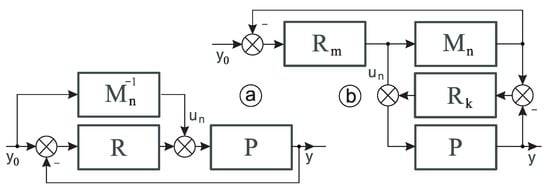
Figure 1. The well-known feedforward structure (a) and the model-following control (MFC) system (b).

The classic single-loop PID control shows some natural robustness to variations of process parameters and structures [30]. This property is widely used to generate non-linear control. However, exceeding the limits of robustness results in control quality degradation.

It would be interesting to multiply the robustness of PID control by increasing the number of loops. To do this, let us assume that the forward process model $M_n$ has scalable complexity (1):

$$\begin{array}{c}\hfill \left\{\begin{array}{c}{M}_1={\tilde{M}}_1(1+{\Delta }_1)\hfill \\ M_2={\tilde{M}}_1(1+{\Delta }_1)+{\tilde{M}}_2(1+{\Delta }_2)\hfill \\ ...\hfill \\ M_i={\tilde{M}}_1(1+{\Delta }_1)+{\tilde{M}}_2(1+{\Delta }_2)+...+{\tilde{M}}_i(1+{\Delta }_i)\hfill \\ ...\hfill \\ M_n={\tilde{M}}_1(1+{\Delta }_1)+{\tilde{M}}_2(1+{\Delta }_2)+...+{\tilde{M}}_i(1+{\Delta }_i)+...+{\tilde{M}}_n(1+{\Delta }_n)\hfill \end{array}\right.\end{array}$$

(1)

where $M_i$ are non-linear parts of the whole process model $M_n$. Additionally, ${\tilde{M}}_i$ represents the linear components of the model and corresponding ${\Delta }_i$ multiplicative perturbations. As will be shown in the simulation section, the non-linear forward process model $M_n$ can be presented in the form of a gradation of complexity $M_i$. If this condition is met, a multi-model structure can be introduced which is composed of classic PID loops (Figure 2). The mechanism of the proposed system is very simple and is based on a stepwise linearization that finally leads to the determination of a global non-linear control variable $u_n$. Starting from the first loop, the $R_1$ is the controller of the simplest model $M_1$, generating the first component of the non-linear value $u_1$. The measured model variable $y_1$ is also the setpoint value for the second loop in which $M_2$ is included. The $R_2$ follows the $y_1$, generating an additional corrective value next to the $u_1$, which finally forms the control value $u_2$. Each following loop generates the additional non-linear component of the control value $u_i$. The number of loops used is determined by the complexity of the model $M_n$. The individual $M_i$ models should be prepared to benefit as much as possible from the natural robustness of a single PID loop. Please note that using an over-complex model $M_i$ may lead to a degradation of the control quality $y_i$, which will automatically degrade the next loop.

$$y_n=y_0\frac{R_1{M}_n}{1+R_1{M}_1}\frac{{\displaystyle \prod _{i=2}^n}(1+R_i{M}_{i-1})}{{\displaystyle \prod _{i=2}^n}(1+R_i{M}_i)}$$

(2)

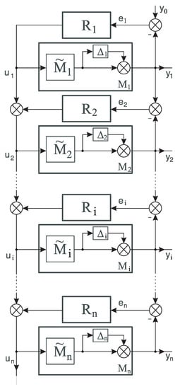
Figure 2. The general form of the multi-loop linearization concept.

The proposed multi-loop structure is based on a multiplication of the single-loop PID control. This greatly simplified the stability and robustness analysis, which is presented in the next subsection. Equation (2) describes the transfer function of the multi-loop structure in Figure 2.

2.1. Stability

The system under consideration is composed, in general, of n-loops that contain the non-linear components of the process model $M_i$ and corresponding PID controllers $R_i$ that generate the non-linear control values. The proper operation of the proposed method is provided by satisfying the stability condition. Looking at the multi-loop structure, it is clear that its basic component includes a single PID loop. Thus, it can be expected that the global stability of the Figure 2 structure will depend on the local stability of each loop. We will assume that the models $M_i$ are linear and time-invariant. The stability conditions of the last loop are based on the analysis of the error $e_n$, which can be described as $e_n=y_{n-1}-y_n$, where $y_{n-1}=u_{n-1}{M}_{n-1}$ and $y_n=(u_{n-1}+e_n{R}_n)M_n$. After the respective transformation, we obtain

$$e_n=\frac{{\displaystyle u_{n-1}(M_{n-1}-M_n)}}{{\displaystyle 1+M_n{R}_n}}$$

(3)

Let the elements of Equation (3) be given in a rational form: $u_{n-1}=\frac{n_1}{d_1}$, $R_n=\frac{n_2}{d_2}$, $M_{n-1}=\frac{n_3}{d_3}$, $M_n=\frac{n_4}{d_4}$. Substituting into (3) yields

$$e_n=\frac{{\displaystyle n_1{d}_2(n_3{d}_4-n_4{d}_3)}}{{\displaystyle d_1{d}_3(d_2{d}_4+n_2{n}_4)}}$$

(4)

The characteristic equation $d_1{d}_3(d_2{d}_4+n_2{n}_4)=0$ presents the required conditions for the considered system to be stable. The part $(d_2{d}_4+n_2{n}_4)$ is a well-known stability condition for a one-loop PID system, where polynomials are of Hurwitz-type, i.e., their poles have negative real parts. This means that the stability of the structure in Figure 2 consists not only of the stability of the last loop but also of the stability of each of the models $M_i$, as well as of the individual control signals $u_i$, which are described by the equation below:

$$u_{n-1}=y_0\frac{R_1}{1+R_1{M}_1}\frac{{\displaystyle \prod _{i=2}^{n-1}}(1+R_i{M}_{i-1})}{{\displaystyle \prod _{i=2}^{n-1}}(1+R_i{M}_i)}forn>1$$

(5)

2.2. Robustness Analysis

Studying the robustness of control systems is not a trivial task and often involves techniques such as [31,32]. Since the proposed solution duplicates the classic PID system, it is helpful to focus attention on the robustness of the single-loop structure. The variation of process parameters, caused by non-linearity or time-variant behavior, can be modeled by additive or multiplicative perturbation [33]. We will focus on one of them, i.e., the multiplicative perturbation, which is defined as $P=\tilde{P}(1+{\Delta }_p)$, where P is the non-linear representation of the plant, $\tilde{P}$ the linear representation of the plant, and ${\Delta }_p$ the multiplicative perturbation. For such an adopted description, the robustness of the classic one-loop structure is described by the formula [34]

$$\begin{array}{c}\hfill {\left|{\Delta }_p\left(j\omega \right)\right|}_{pid}<\left|\frac{{\displaystyle 1+R\left(j\omega \right)\tilde{P}\left(j\omega \right)}}{{\displaystyle R\left(j\omega \right)\tilde{P}\left(j\omega \right)}}\right|\end{array}$$

(6)

We could use the above formula directly if we could transform the multi-loop structure of Figure 2 to an equivalent single-loop form. Since the first loop with model $M_1$ is an independent loop, we will start the transformation from the second loop. If the number of models in the structure is n > 1, additional robustness introduced by model loops should be considered. In Figure 3, the multi-loop structure has been transformed to the equivalent single-loop form by introducing additional blocks $G_1$ and $G_2$. The transfer function for the equivalent system has the form

$$y_i=\frac{R_2{M}_i{G}_1}{1+R_2{M}_i{G}_2}{y}_{1}forn>1$$

(7)

where

$$\begin{array}{ccc}\hfill G_1& =& \frac{{\displaystyle \prod _{i=3}^n}(1+R_i{M}_{i-1})}{{\displaystyle \prod _{i=3}^n}(1+R_{i-1}{M}_{i-1})}\hfill \end{array}$$

(8)

$$\begin{array}{ccc}\hfill G_2& =& \frac{R_i}{R_2}\hfill \end{array}$$

(9)

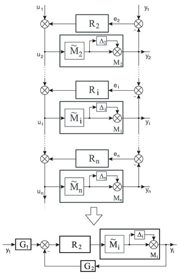
Figure 3. Model loops with a multiplicative uncertainty and its reduction to the classic PID structure.

For the modified structure shown in Figure 3, we can directly apply the robustness condition for the single-loop system (6), which takes the form

$$\begin{array}{ccc}\hfill \left|{\Delta }_i\right|& <& \left|\frac{1+R_2\widetilde{M_i}{G}_2}{R_2\widetilde{M_i}}\right|\hfill \end{array}$$

(10)

By substituting (8) and (9), we finally obtain the condition for allowable perturbations:

$$\begin{array}{ccc}\hfill \left|{\Delta }_1\right|& <& \left|\frac{1+R_1\widetilde{M_1}}{R_1\widetilde{M_1}}\right|forn=1\hfill \end{array}$$

(11)

$$\begin{array}{ccc}\hfill \left|{\Delta }_i\right|& <& \left|\frac{1+R_i\widetilde{M_i}}{R_2\widetilde{M_i}}\right|forn>1\hfill \end{array}$$

(12)

As expected, inserting additional loops increases the resulting robustness (12) of the whole system. This property can be used to generate the non-linear component of the control variables $u_i$, which ultimately comprise the global non-linear control value $u_n$.

3. Results

The main goal of the simulation study is to confirm that the proposed forward model-based system is also capable of generating strong non-linear control value such as the feedforward structure based on the inverse model. It was quite a challenge to select the right process for the simulation study. A key selection criterion was the analytical ability to determine both the forward and the inverse model. In addition, the high complexity of the process was to illustrate the point of using a multi-loop structure with scalable forward model complexity. A two-joint serial manipulator with force interaction was finally selected (Figure 4).

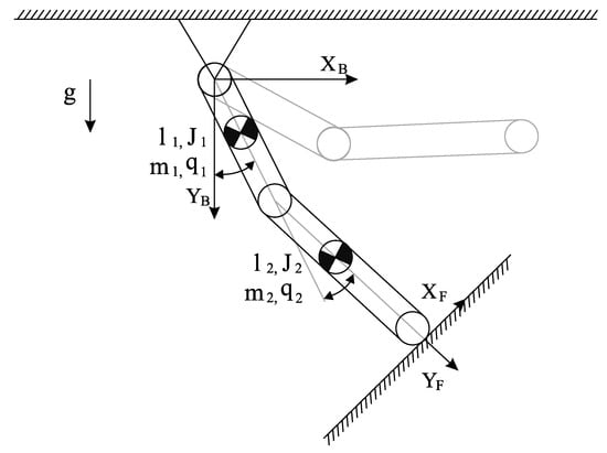
Figure 4. The 2DOF manipulator with force interaction.

From a position control perspective alone, an industrial manipulator is an extremely complex process. Strong static and dynamic non-linearities and time-variant behavior go far beyond the robustness of a single-loop PID control [35]. The additional robot interaction with the environment introduces further non-linearities into the control system [36]. Regardless of the method used to identify the robot’s dynamic (Euler–Lagrange or Newton–Euler formulation) [37], the mathematical model including force interaction with the environment has the following form:

$$\begin{array}{c}\hfill M\left(q\right)\ddot{q}+C(q,\dot{q})+G\left(q\right)+D\left(\dot{q}\right)=\tau -J^T\left(q\right)F\end{array}$$

(13)

We will use a 2DOF manipulator for the simulation purposes. For this case, the elements of Equation (13) take the form

$$\begin{array}{c}M\left(q\right)=\left[\begin{array}{cc}(m_1+m_2)l_1^2+m_2{l}_2^2+2m_2{l}_1{l}_2{c}_2+J_1& m_2{l}_2^2+m_2{l}_1{l}_2{c}_2\\ m_2{l}_2^2+m_2{l}_1{l}_2{c}_2& m_2{l}_2^2+J_2\end{array}\right]\hfill \\ \\ C(q,\dot{q})=\left[\begin{array}{c}-m_2{l}_1{l}_2{s}_2{\dot{q}}_2^2-2m_2{l}_1{l}_2{s}_2{\dot{q}}_1{\dot{q}}_2\\ m_2{l}_1{l}_2{s}_2{\dot{q}}_1^2\end{array}\right]\hfill \\ \\ G\left(q\right)=\left[\begin{array}{c}g(m_1{l}_1{c}_1+m_2{l}_1{c}_1+m_2{l}_2{c}_{12})\\ g{m}_2{l}_2{c}_{12}\end{array}\right]\hfill \\ \\ D\left(\dot{q}\right)=\left[\begin{array}{c}0.8sig\left(\dot{q_1}\right)\\ 0.3sig\left(\dot{q_2}\right)\end{array}\right],J^T\left(q\right)=\left[\begin{array}{cc}-l_1{s}_1-l_2{s}_{12}& l_1{c}_1+l_2{c}_{12}\\ -l_2{s}_{12}& l_2{c}_{12}\end{array}\right]\hfill \end{array}$$

(14)

M(q) is the n × n inertia matrix, $C(q,\dot{q})$ is the n × 1 vector of centrifugal and Coriolis terms, G(q) is the n × 1 vector of gravitational effects, $D\left(\dot{q}\right)$ is the n × 1 vector of viscous friction, $\tau$ is the n × 1 vector of actuator torques, and $\ddot{q},\dot{q},q$ are the n × 1 vectors of acceleration, velocity, and position, respectively. The n × m matrix $J^T\left(q\right)$ is the transpose of the Jacobian of the robot, and F is the m × 1 vector of the force that the (m-dimensional) environment exerts at the contact point. Additionally, $s_{12}=sin(q_1+q_2), c_{12}=cos(q_1+q_2), m_1=20.7\mathrm{kg}, m_2=2.2\mathrm{kg}, l_1=0.5\mathrm{m}, l_2=0.7\mathrm{m}, J_1=1.85{\mathrm{kgm}}^2, J_2=1.6{\mathrm{kgm}}^2$, g is the acceleration of gravity. The above parameters represent the EDDA (experimental direct drive arm), a real 2DOF manipulator, which has been discussed in many scientific publications [38,39]. From a simulation point of view, the maximum torque of the direct drives used is an important piece of information. Reluctance motors generate the torques, respectively, ${\tau }_1=\pm 250\mathrm{Nm}$ and ${\tau }_2=\pm 40\mathrm{Nm}$. These constraints were introduced into the simulation to better represent the behavior of the real process.

3.1. Preparation of Non-Linear Process Models

Access to the inverse model will help us compare the proposed system to the well-known feedforward control. However, to simulate the structure of Figure 2, it is necessary to determine the forward process model. Since the matrix M(q) is invertible for all q, the Equation (13) can be easily transformed to the form

$$\begin{array}{c}\hfill \ddot{q}=M{\left(q\right)}^{-1}[\tau -C(q,\dot{q})-G\left(q\right)-D\left(\dot{q}\right)-J^T\left(q\right)F]\end{array}$$

(15)

Of course, the physical implementation of the model (15) requires the use of double integration to determine the missing state variables q and $\dot{q}$. This is, along with the other methods [40], one of the most classic approaches to the practical determination of a forward dynamic model of a robot manipulator. To demonstrate the significance of the proposed concept with forward model scalability, we perform a simple simulation comparing the performance of both control structures presented in Figure 1. Equation (13) was used as an inverse model $M_n^{-1}$ for the feedforward system (a), while Equation (15) as a forward model $M_n$ was applied to the MFC structure (b).

The PID controllers have been tuned to achieve the best possible results for different setpoint values. Equation (15) represents the process P for both feedforward and MFC structures. Figure 5 and Figure 6 illustrate the quality of position control for the first and the second joint, respectively. In this comparison, the feedforward system offers a very good quality of control. It is difficult to expect different results if the compensator $M_n^{-1}$ is the perfect inverse of the process P. However, for the MFC structure, the control quality is very poor. The reason for this is the limited robustness of a single PID loop that contains a strongly non-linear forward model $M_n$. This example perfectly demonstrates the constraints of the MFC system, which became the motivation for using a multi-loop technique with scalable forward model complexity.

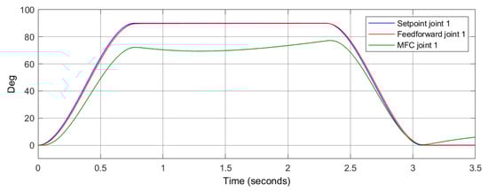
Figure 5. The performance of position control for the feedforward and MFC structure—joint 1.

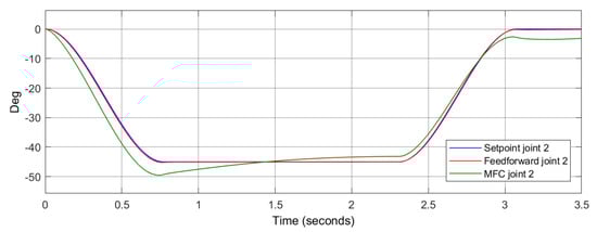
Figure 6. The performance of position control for the feedforward and MFC structure—joint 2.

Equation (15) represents the total process model. The $M_i$ models should be chosen in such a way that, on the one hand, good control quality in each loop is assured and, on the other hand, the robustness of the PID control is maximally utilized. For simulation purposes, the following gradation of model complexity was proposed:

$$\begin{array}{c}\hfill \begin{array}{c}{M}_1:\ddot{q}=M{\left(q\right)}^{-1}[\tau -C(q,\dot{q})-D\left(\dot{q}\right)]\hfill \\ M_2:\ddot{q}=M{\left(q\right)}^{-1}[\tau -C(q,\dot{q})-D\left(\dot{q}\right)-G\left(q\right)]\hfill \\ M_3:\ddot{q}=M{\left(q\right)}^{-1}[\tau -C(q,\dot{q})-D\left(\dot{q}\right)-G\left(q\right)-J^T\left(q\right)F]\hfill \end{array}\end{array}$$

(16)

The forward models presented in (16) show the simplicity of practical implementation of the proposed method. Based on the simulation, the number of required loops can be optimally selected. In this case, it was decided to use three loops in the configuration shown in Figure 2.

Since the feedforward structure will be the reference point in evaluating the performance of the proposed system, the following inverse models will be used in the simulation:

$$\begin{array}{c}\hfill \begin{array}{c}{M}_1^{-1}:\tau =M\left(q\right)\ddot{q}+C(q,\dot{q})+D\left(\dot{q}\right)\hfill \\ M_2^{-1}:\tau =M\left(q\right)\ddot{q}+C(q,\dot{q})+D\left(\dot{q}\right)+G\left(q\right)\hfill \\ M_3^{-1}:\tau =M\left(q\right)\ddot{q}+C(q,\dot{q})+D\left(\dot{q}\right)+G\left(q\right)+J^T\left(q\right)F\hfill \end{array}\end{array}$$

(17)

3.2. Simulation Study

For simulation purposes, the Matlab/Simulink environment was used. All models presented in (16) and (17) were implemented in C language in the form of S-Function. To show the performance of the presented system, feedforward control was implemented for comparison purposes. The forward models (16) were used to build and simulate the structure from Figure 2, while the inverse models (17) allowed adequate feedforward structures from Figure 1a to be prepared. The setpoint value for the first joint was $y_0={90}^{\circ }$ and for the second joint was $y_0=-{45}^{\circ }$. After 2.3 s, the setpoint value was changed to $y_0=0^{\circ }$ for both joints. The setpoint values were generated using a third-order polynomial. This was required by inverse models (17), which need all three variables, $q,\dot{q},\mathrm{and} \ddot{q}$, to determine the control value.

The simulation was started from the simplest case, i.e., from models $M_1$ and $M_1^{-1}$. Figure 7b and Figure 8b show the non-linear control value generated by the feedforward system and the structure from Figure 2 (single PID loop). In this case, the models $M_1$/$M_1^{-1}$ do not include the effects of gravity and force interaction with the environment. Switching to a model that takes into account the effects of gravity $M_2$/$M_2^{-1}$, the structure in Figure 2 takes a two-loop form. For this case, Figure 9b and Figure 10b show the comparison of the non-linear control value. A final test was performed for the most complex models $M_3$/$M_3^{-1}$. For the non-linear interaction with the environment, the force vector was defined as $F={\left[5050\right]}^T$. In this case, the structure in Figure 2 took a three-loop form. Figure 11b and Figure 12b show the comparison of the non-linear control value. The small differences observed in the generated control signals compared to the feedforward are a result of the way the non-linear values are determined. The feedforward method is called the direct linearization technique, because the control value is calculated directly from the inverse model. Another approach is used in the proposed multi-model system and is called the indirect linearization method. In this case, the control value is computed indirectly in feedback loops.

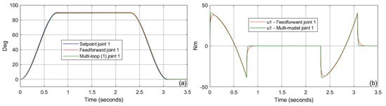
Figure 7. Comparison of position control quality (a) and corresponding control value (b)—case $M_1$/$M_1^{-1}$, joint 1.

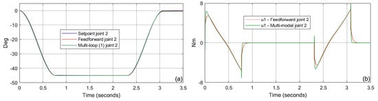
Figure 8. Comparison of position control quality (a) and corresponding control value (b)—case $M_1$/$M_1^{-1}$, joint 2.

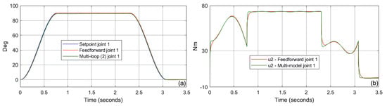
Figure 9. Comparison of position control quality (a) and corresponding control value (b)—case $M_2$/$M_2^{-1}$, joint 1.

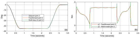
Figure 10. Comparison of position control quality (a) and corresponding control value (b)–case $M_2$/$M_2^{-1}$, joint 2.

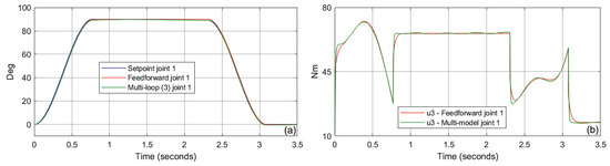
Figure 11. Comparison of position control quality (a) and corresponding control value (b)—case $M_3$/$M_3^{-1}$, joint 1.

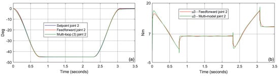
Figure 12. Comparison of position control quality (a) and corresponding control value (b)—case $M_3$/$M_3^{-1}$, joint 2.

Finally, we should look at the control quality that can be achieved with the presented technique. Figure 7, Figure 8, Figure 9, Figure 10, Figure 11 and Figure 12a show the following of the setpoint value for the compared systems. As might be expected, the feedforward structure follows the setpoint value $y_0$ perfectly. However, considering the scale of the complexity of the process, the presented approach generates interesting results as well. The significance of using the multi-loop technique is perfectly illustrated by comparing Figure 5 and Figure 6 with Figure 11a and Figure 12a. In this case we are looking at the most complex process described by the models (13) and (15). The use of scalable forward models (16) plugged into a three-loop structure (Figure 2) allows for a significant improvement in control quality.

4. Conclusions

In this paper, the multi-loop structure based on the forward process models was presented. The scalable model complexity technique makes it possible to effectively use the natural robustness of the PID control. Based on the position control of a robot manipulator with environment interaction, the capability of generating non-linear control values was compared to the feedforward structure. In this complex process, simultaneous access to the inverse and forward model greatly simplified the simulation studies. However, it should be noted here that the reason for using this proposed solution is when the determination of the inverse process model is difficult or impossible, which is mostly the case.

We should look at the practical implementation of the proposed solution. The combination of multiple loops along with specially prepared models may make it seem difficult to use this system in practice. However, as the simulation section shows, the synthesis of the multi-model structure is not significantly challenging. Since the basic component of the structure is nevertheless a well-known single PID loop, this greatly simplifies the implementation and tuning process. Of course, the proposed system also requires adequate computing power. However, this is not a critical condition. Similar to the feedforward approach, it is also possible to calculate the non-linear control value in the off-line mode. The proposed system is an interesting alternative to the classical compensator design, based on the inverse model. The presented method opens new possibilities of control of strongly non-linear processes for which determination of the inverse model is impossible.

References

- Agachi, P.S.; Nagy, Z.K.; Cristea, M.V.; Imre-Lucaci, Á. Model Based Control: Case Studies in Process Engineering; Wiley-VCH Verlag GmbH & Co. KGaA: Hoboken, NJ, USA, 2006. [Google Scholar]
- Francis, B.A.; Wonham, W.M. The internal model principle of control theory. Automatica 1976, 10, 457–465. [Google Scholar] [CrossRef]
- Shao, L.; Liu, C.; Wang, Z.; Wang, J.; Yang, X. The Temperature Control of Blackbody Radiation Source Based on IMC-PID. In Proceedings of the Conference on Mechatronics and Automation, Tianjin, China, 4–7 August 2019; pp. 1698–1702. [Google Scholar]
- Arya, P.P.; Chakrabarty, S. Robust internal model controller with increased closed-loop bandwidth for process control systems. IET Control Theory Appl. 2020, 14, 2134–2146. [Google Scholar] [CrossRef]
- Li, P.; Zhu, G.; Zhang, M. Linear Active Disturbance Rejection Control for Servo Motor Systems With Input Delay via Internal Model Control Rules. IEEE Trans. Ind. Electron. 2021, 68, 1077–1086. [Google Scholar] [CrossRef]
- Alfaro, V.M.; Vilanova, R.; Arrieta, O. Analytical robust tuning of PI controllers for first-order-plus-dead-time processes. In Proceedings of the Conference on Emerging Technologies & Factory Automation, Hamburg, Germany, 15–18 September 2008; pp. 273–280. [Google Scholar]
- Åström, K.J.; Hang, C.C.; Lim, B.C. A new Smith predictor for controlling a process with an integrator and long dead-time. IEEE Trans. Autom. Control. 1994, 39, 343–345. [Google Scholar] [CrossRef] [Green Version]
- Zhu, Q.; Yin, Z.; Zhang, Y.; Niu, J.; Li, Y.; Zhong, Y. Research on Two-Degree-of-Freedom Internal Model Control Strategy for Induction Motor Based on Immune Algorithm. IEEE Trans. Ind. Electron. 2016, 63, 1981–1992. [Google Scholar] [CrossRef]
- Cui, J.; Wang, Z.; Chen, Y.; Liu, T. Indirect iterative learning control design based on 2DOF IMC for batch processes with input delay. In Proceedings of the Conferen Chinese Control Conference, Dalian, China, 26–28 July 2017; pp. 3587–3592. [Google Scholar]
- Mikulas, H.; Bistak, B.; Vrancic, D. 2DOF IMC and Smith-Predictor-Based Control for Stabilised Unstable First Order Time Delayed Plants. Mathematics 2021, 9, 1064. [Google Scholar]
- Siciliano, B.; Khatib, O. Springer Handbook of Robotics; Springer: Berlin/Heidelberg, Germany, 2008. [Google Scholar]
- Mahmoud, M.S.; Xia, Y. Applied Control Systems Design; Springer: Berlin/Heidelberg, Germany, 2012. [Google Scholar]
- Roffel, B.; Betlem, B.H. Advanced Practical Process Control; Springer: Berlin/Heidelberg, Germany, 2004. [Google Scholar]
- Commercial Modelica Simulation Environments. Available online: https://www.modelica.org/tools (accessed on 9 September 2021).
- Looye, G.; Thuemmel, M.; Kurze, M.; Otter, M.; Bals, J. Nonlinear Inverse Models for Control. In Proceedings of the Conference International Modelica Conference, Hamburg, Germany, 7–8 March 2005; pp. 267–279. [Google Scholar]
- Li, G.; Tsang, K.M.; Ho, S.L. A novel model following scheme with simple structure for electrical position servo systems. Int. J. Syst. Sci. 1998, 29, 959–969. [Google Scholar] [CrossRef]
- Osypiuk, R. Simple robust control structures based on the model-following concept—A theoretical analysis. Int. J. Robust Nonlinear Control 2010, 20, 1920–1929. [Google Scholar] [CrossRef]
- Shibasaki, H.; Yusof, R.; Ishida, Y. A Design Method of a Model-following Control System. Int. J. Control Autom. Syst. 2015, 13, 843–852. [Google Scholar] [CrossRef]
- Skoczowski, S. The Robust Control System With Use of Nominal Model of Controlled Plant. IFAC Proc. Vol. 2000, 33, 911–916. [Google Scholar] [CrossRef]
- Li, G.; Tsang, K.M.; Ho, S.L. Robust Fine Tuning of Optimal PID Controller With Guaranteed Robustness. IEEE Trans. Ind. Electron. 2019, 67, 4911–4920. [Google Scholar]
- Ortega, R.; Loría, A.; Nicklasson, P.J.; Sira-Ramírez, H. Passivity-Based Control of Euler-Lagrange Systems; Mechanical, Electrical and Electromechanical Applications; Springer: Berlin/Heidelberg, Germany, 1998. [Google Scholar]
- Shao, K.; Tang, R.; Xu, F.; Wang, X.; Zheng, J. Adaptive sliding mode control for uncertain Euler—Lagrange systems with input saturation. J. Frankl. Inst. 2021, 358, 8356–8376. [Google Scholar] [CrossRef]
- Aranovskiy, S.; Ryadchikov, I.; Nikulchev, E.; Wang, J.; Sokolov, D. Experimental Comparison of Velocity Observers: A Scissored Pair Control Moment Gyroscope Case Study. IEEE Access 2020, 8, 21694–21702. [Google Scholar] [CrossRef]
- Aranovskiy, S.; Ryadchikov, I.; Nikulchev, E.; Wang, J.; Sokolov, D. Bias Propagation and Estimation in Homogeneous Differentiators for a Class of Mechanical Systems. IEEE Access 2020, 8, 19450–19459. [Google Scholar] [CrossRef]
- Siciliano, B.; Villani, L. Robot Force Control; Springer: Berlin/Heidelberg, Germany, 2013. [Google Scholar]
- Lynch, K.M.; Park, F.C. Modern Robotics: Mechanics, Planning, and Control; Cambridge University Press: Cambridge, UK, 2017. [Google Scholar]
- Ye, H. Stabilization of Uncertain Feedforward Nonlinear Systems With Application to Underactuated Systems. IEEE Trans. Autom. Control 2019, 64, 3484–3491. [Google Scholar] [CrossRef]
- Liu, J.; He, J.; Ho-Ching, I.H. Realization of Low-Voltage and High-Current Rectifier Module Control System Based on Nonlinear Feed-Forward PID Control. Electronics 2021, 10, 2138. [Google Scholar] [CrossRef]
- Roffel, B.; Betlem, B. Process Dynamics and Control: Modeling for Control and Prediction; Wiley: Hoboken, NJ, USA, 2007. [Google Scholar]
- Zhao, C.; Guo, L. Control of Nonlinear Uncertain Systems by Extended PID. IEEE Trans. Autom. Control 2021, 66, 3840–3847. [Google Scholar] [CrossRef]
- Silva, G.J.; Datta, A.; Bhattacharyya, S.P. On the stability and controller robustness of some popular PID tuning rules. IEEE Trans. Autom. Control 2003, 48, 1638–1641. [Google Scholar] [CrossRef]
- Mercader, P.; Åström, K.J.; Baños, A.; Hägglund, T. Robust PID Design Based on QFT and Convex—Concave Optimization. IEEE Trans. Control. Syst. Technol. 2017, 25, 441–452. [Google Scholar] [CrossRef]
- Hagiwara, T.; Araki, M. Robust stability of sampled-data systems under possibly unstable additive/multiplicative perturbations. IEEE Trans. Autom. Control 1998, 43, 1340–1346. [Google Scholar] [CrossRef]
- Skoczowski, S.; Domek, S.; Pietrusewicz, K.; Broel-Plater, B. A method for improving the robustness of PID control. IEEE Trans. Ind. Electron. 2005, 52, 1669–1676. [Google Scholar] [CrossRef]
- Miller, R.K. Industrial Robot Handbook; Springer: New York, NY, USA, 2014. [Google Scholar]
- Gonzalez, J.J.; Widmann, G.R. Investigation of nonlinearities in the force control of real robots. IEEE Trans. Syst. Man. Cybern. 1992, 22, 1183–1193. [Google Scholar] [CrossRef]
- Spong, M. Robot Modeling and Control; John Wiley and Sons Ltd.: Hoboken, NJ, USA, 2020. [Google Scholar]
- Osypiuk, R.; Finkemeyer, B.; Skoczowski, S. Simple two degree of freedom structures and their properties. Robotica 2006, 24, 365–372. [Google Scholar] [CrossRef]
- Kozłowski, K. Modelling and Identification in Robotics; Springer: Berlin/Heidelberg, Germany, 2012. [Google Scholar]
- Kvrgic, V.; Vidakovic, J. Efficient method for robot forward dynamics computation. Mech. Mach. Theor. 2020, 145, 103680. [Google Scholar] [CrossRef]
Publisher’s Note: MDPI stays neutral with regard to jurisdictional claims in published maps and institutional affiliations. |
© 2021 by the author. Licensee MDPI, Basel, Switzerland. This article is an open access article distributed under the terms and conditions of the Creative Commons Attribution (CC BY) license (https://creativecommons.org/licenses/by/4.0/).