Article

Estimation and Interpretation of Machine Learning Models with Customized Surrogate Model

1
Department of Computer Science, COMSATS University Islamabad, Islamabad 44000, Pakistan
2
College of Technological Innovation, Zayed University, Abu Dhabi 19282, United Arab Emirates
3
Department of Electrical Engineering, HITEC University, Taxila 47080, Pakistan
4
Institute of Management Sciences Peshawar, Peshawar 25100, Pakistan
5
Department of Computer Science and Engineering, University of Engineering and Technology, Norowal Campus, Lahore 54890, Pakistan
6
School of Computing, Engineering and Physical Sciences, University of the West of Scotland, Paisley PA1 2BE, UK
7
Department of Computer Science, Federal Urdu University of Arts, Science and Technology, Islamabad 44000, Pakistan
8
Department of Software, Yonsei University, Wonju 26493, Korea
9
Department of Computer Science and Engineering, Chungnam National University, Daejeon 34134, Korea
*
Author to whom correspondence should be addressed.
Electronics 2021, 10(23), 3045; https://doi.org/10.3390/electronics10233045
Submission received: 15 October 2021 / Revised: 2 December 2021 / Accepted: 3 December 2021 / Published: 6 December 2021

Abstract

:
Machine learning has the potential to predict unseen data and thus improve the productivity and processes of daily life activities. Notwithstanding its adaptiveness, several sensitive applications based on such technology cannot compromise our trust in them; thus, highly accurate machine learning models require reason. Such models are black boxes for end-users. Therefore, the concept of interpretability plays the role if assisting users in a couple of ways. Interpretable models are models that possess the quality of explaining predictions. Different strategies have been proposed for the aforementioned concept but some of these require an excessive amount of effort, lack generalization, are not agnostic and are computationally expensive. Thus, in this work, we propose a strategy that can tackle the aforementioned issues. A surrogate model assisted us in building interpretable models. Moreover, it helped us achieve results with accuracy close to that of the black box model but with less processing time. Thus, the proposed technique is computationally cheaper than traditional methods. The significance of such a novel technique is that data science developers will not have to perform strenuous hands-on activities to undertake feature engineering tasks and end-users will have the graphical-based explanation of complex models in a comprehensive way—consequently building trust in a machine.

1. Introduction

Machine learning, a substitute for artificial intelligence, is a pivotal part of modern computer society. It involves scientific and algorithmic techniques that are specifically designed to curb user involvement and thus increase the automaticity of the desired work. Nowadays, most computer systems are built for performing general or business-specific tasks through machine learning technologies. Evidence of their applications can be seen in problem domains such as in the medical field, policy-making [1], fraud detection [2,3,4], and signal processing [5,6]. Different machine learning models, also known as mathematical models, possess different attributes that produce accurate results using prediction calculations when exposed to a given dataset. Many accurate decision support systems have been built as black boxes in recent years, i.e., systems that hide their internal logic from the end- user during the estimation process that containing dozens of parameters and other complex formulations for making predictions.
A black box model can either be a function that is excessively complex for humans to understand or a function in whose noisy data are extremely difficult for humans to uncover, potentially leading to incorrect predictions. Deep learning models, gradient boosting or random forest are extremely recursive in nature which is why they are called black box models. Here, an explanation is a distinct model that is expected to duplicate most of the behavior of a black box, which is the most popular sense in which the term is currently used; in this research, however, the term explanation refers to an understanding of how a model of machine learning systems works [7].
Interpretable machine learning refers to machine learning models that can provide explanations regarding why certain predictions are made. This is also known as white box/glass box models which are comparatively much easier to understand and audit than complex/black box models. Traditional machine learning metrics such as AUC, accuracy and recall may not be sufficient in many applications where user trust in a machine’s predictions is required. Although there is no mathematical definition of interpretability, [8] found that ’Interpretability is the degree to which a human can understand the cause of a decision’. Similarly, [9] found that ’Interpretability is the degree to which a human can consistently predict the model’s result’. Thus, to summarize the previous statements, one can say that if a machine learning model has higher interpretability, then comprehending the behavior behind the prediction that the black box model has made will be easier. Generally, there are two categories of interpretable approaches: one focuses on personalized interpretation, a situation in which the specific prediction of a specific instance is interrogated, called local interpretability, while the second summarizes prediction models at a population level which means that we can understand the whole logic and reasoning of an entire model consisting of all possible outcomes—what we call global interpretability [10].
In this article, black box models refer to models that are not directly understandable by the end-user which are complex due to a large number of parameters or rules involved that give it higher accuracy. In contrast, simple models are models that comprise fewer parameters or have less rules (tree-based classifiers with medium depth), thus enabling the end-user to understand and adjust them according to their rationales; these are considered easily understandable by humans. If we specify examples of complex models, these include: random forest (RF) [11]; support vector machines (SVMs) [12]; gradient boosting (GB) [13]; deep neural networks (DNNs) [14,15]. Meanwhile, simple/glass box/white box models (sometimes called interpretable models [16]) include decision trees (DT) [17]; and linear regression (LR)/logistic regression (LOR) [18].
There are several sensitive applications [19,20,21,22] for which an explanation behind the prediction is essential. Therefore, in the absence of explanation, no one can simply rely on machines. Another downfall of using is the possibility of making the drawing an incorrect prediction from the artifacts (data), thus affecting the overall performance of the machine’s efficiency [23].
The availability of transparency in machine learning predictions could foster awareness of and some level of trust in machines. Moreover, the trade-off factor between the interpretability and accuracy of the model while mimicking the black box models for an explanation is indeed another gap to address when explaining the complex/black box models—b. Sometimes, such tasks are computationally expensive as well.
This research work focuses on explaining the black box model via some available interpretable methods without compromising the accuracy of the black box for multiple problem domains such as classification and regression. This will eventually gain the trust of the end-user. This requires some methodology that contains certain mathematical techniques which will assist us in performing multiple tasks at a time. These tasks include dealing with trade-off factors as mentioned earlier, automatic feature engineering tasks for feature transformation and mimicking the underlying black box model in a way that is directly comprehensible by humans as an explanation.
For the sake of the transparency of the black box, we follow these two most important concerns in a machine learning paradigm. First, describing how black box models work (capturing the behavior) and secondly, explaining that captured behavior in human-understandable language. In brief, we can say that explanation is the core priority for describing how a black box model works. In this research work, we denote the complex/black box as b. b is an obscure machine learning and data mining model whose inner working is unknown—or if it is known, then it is not understandable by humans. To interpret means to provide an explanation or meaning and present it in human-understandable terms. Hence, machine learning models are interpretable models when b is complex in nature but understandable by humans. Thus, if these conditions are satisfied, then the underlying machine learning model is interpretable. Interpretable models, henceforth, build trust and encourage users to use them to take decisions according to what the machine has estimated. After considering the previous statements, we achieved results with higher accuracy that were also interpretable. The technique we propose is capable of acknowledging both the regression and classification problem domains.
Explainability is usually referred to as an interface between the decision maker and humans that is an accurate proxy and comprehensible by humans at the same time. Comprehensibility means that humans can understand why the machine has made a specific prediction and what specific prediction it has made before taking decisions accordingly, which means that if any changes are required, then humans can easily incorporate them after knowing the reasoning behind the predictions. (We will be interchangeably using the term comprehensibility with interpretability in this work.) Thus, the main motivation behind a such research work was to make a black box model (in which the internal behavior is almost impossible to trace) interpretable/auditable/understandable/explainable/comprehensible [24].
Now, coming to the general problem formulation for the interpretable machine learning model paradigm, the predictor could mathematically be defined as
b : X ( m ) Y
where b is the predictor/black box model which allows the mapping of tuples x from a feature space X ( m ) along with m inputs to decision y in a target space Y. We can write b ( x ) = y as a decision made by a p r e d i c t o r b. Thus, b is basically a target to model in order to interpret how the model is making predictions upon a given dataset D m n . In supervised learning, the predictor b is trained on data D t r a i n and then evaluated upon feeding test data D t e s t . The accuracy is then measured on the basis of matches between y ^ D t e s t and y D t r a i n . If the difference between them is the lowest or equal to none, then model b is efficient in its performance.
The factor that contributes in model interpretation is the interpretable predictor C which is processed with the motivation that it will yield a decision C g l o b a l x for a symbolic interpretation understandable/comprehensible by humans. The extent to which C is accurate can be determined by comparing the accuracy of both b and C over D t e s t and secondly fidelity, which evaluates that how well C has mimicked the predictor b upon the given D t e s t . We can formally denote fidelity by
C ( x ) = b ( x ) f o r ( x , y ^ ) D t e s t
Note that C is regarded as interpretable and is also known as the white box model as mentioned earlier.
We then need to understand how the black box b explanation can be practically implemented in a way that would be able to provide a global explanation through an interpretable model C. This means that we need to produce a surrogate model f that can imitate the behavior of b and should be understandable by humans through some explanatory model ε . We can also formalize this problem by assuming that the interpretable global predictor is derived from some dataset of instances X and the black box b. The user will provide some dataset X for the sampling of the domain X ( m ) which may include actual values which will allow the evaluation of the accuracy of the interpretable model. b will thus be trained on dataset X. The process for extracting the interpretable predictor could further expand X. Hence, we can organize the whole model explanation problem as: ‘Given a predictor b and a set of instances X, the surrogate model f assists in explaining via some explanator E   ϵ   ε where ε is the domain directly comprehensible by humans with the help of an interpretable global predictor C g l o b a l = f ( b , X ) that is derived from b and the instances X using some process f(·, ·) as the surrogate function. Then, an explanation E  ϵ   ε is obtained through C g l o b a l , if E = ε g ( C g l o b a l , X ) ’.

1.1. Scope and Objective

To interpret the black box model b, a surrogate function f ( ) , approximates the behavior of b by mimicking it as accurately as possible (or performing even better) in terms of the available performance measurement tools. The methodology includes feature transformation from X to X * . Then, the explanation is produced through an explanator ε g l o b a l which will enable the end-user to comprehend how b is behaving upon giving inputs (features). Henceforth, the main objective of this research is to make the black box model interpretable through a proposed technique that is computationally cheaper than those proposed in previous work(s), supports the automatic feature engineering task, ensures the trade-off between interpretability and accuracy and acknowledges both the classification as well as the regression problem domains. This led us to build a surrogate model that is capable of mimicking and explaining the behavior of the underlying black box model.

1.2. Problem Statements

Comprehending the black box machine learning model’s behavior is difficult which hinders the end-user’s willingness to take further decisions based on the machine’s prediction. If interpretability is achieved, then there is a trade-off between the interpretability and accuracy of a model [25,26] which is another critical problem. According to [27,28], the interpretability of a model decreases if we are not willing to compromise the actual accuracy of the learning model. In other words, these two factors—interpretability and accuracy—are inversely proportional to each other and can be mathematically described as
A M 1 C M g l o b a l
In Equation (3), A denoted accuracy, M is the underlying machine learning model and in this article, we set it as b, as discussed in detail in the previous subsection and C g l o b a l is the interpretation extracted for model M. Furthermore, this problem is also visually described in Figure 1.
The main reason for such setback was the difficulty entailed in exploring and understanding all the parameters involved in providing the higher accuracy A of complex models. The explanation ε g l o b a l of the estimated behavior of b is another cumbersome phase where the explanation is provided or produced by function f is either comprehensible by humans or not. On the other hand, the execution time for approximating [29,30,31] b through C g l o b a l which is approximately equal to { ( x , y ^ )   ϵ   ( D t e s t ) } is indeed another crucial point of the machine learning model’s interpretability while dealing with a large volume of available data. Thus, we can summarize our problem as follows: we need to produce a surrogate function f g l o b a l that can assist in building an interpretation for b through some ε g l o b a l after approximating via C g l o b a l and a blank equation would be:
C g l o b a l f ( b , X ) ε g l o b a l
Finding Equation (4) is the backbone of this whole research. This equation has already been discussed in textual format.

1.3. Research Contribution

  • We considered different datasets from different resources elaborated in Section 4 in which insights into the datasets are provided. Moreover, these datasets belong to both classification and regression problem domains. With the help of the surrogate model, we were able to perform automatic feature engineering tasks. Then, b was mimicked with the assistance of available global surrogate methods (elaborated in Section 3.6)—also known as white box models—before providing an explanation that is comprehensible for end-users. While mimicking the underlying b, in most cases, our proposed methodology outperforms the b which means that we accomplished our objective of retaining the high accuracy of the model and explaining the inner working of b in a way that simultaneously exposes how b acts when exposed to the specific features of the original dataset.
  • There are several areas in which interpretation is necessary because of the legal requirements by target area [32]. Interpretability thus encourages the development of the analysis of interpretable patterns from trained models by allowing one to identify the causes behind poor predictions by machines. If b becomes comprehensible by the end-user, it will surely engender trust in machines and help users detect biasness in machine learning models—as we are doing herein.
  • In this work, we propose a technique called enhanced surrogate-assisted feature engineering (ESAFE) for machine learning models, which is an extension of surrogate-assisted feature extraction for model learning (SAFE ML) [33]. It will address all such issues that general interpretable desiderata (explained in Section 3.1), which requires the incorporation of Equations (1) and (2).
  • With the help of technique [34], the proposed methodology achieved a drastic change in terms of computational cost whilst simultaneously respecting all the constraints mentioned in the interpretable desiderata Section 3.1. This technique will help us build ε g l o b a l . The surrogate model f will assist us in transforming features X ( m ) and thus produce C g l o b a l as a result. With enhanced visual interpretability accurately imitating quality and without compromising the accuracy of the machine learning model, we hereby provide a novel technique in the form of the Python package so that the end-user may be satisfied with its results. This will enable the end-user to ascertain different features of the relationships and their effects on the overall prediction of b.
The significance of such a technique is to assist the end-user in terms of ensuring the explainability of b’s inner workings—rendering it auditable and the data scientist comfortable with skipping the time-consuming process of undertaking a feature engineering task. Therefore, both communities would enjoy ESAFE’s multifaceted features.

1.4. Paper Orientation

This paper is organized as follows. Section 2 discusses related work. The working of the proposed algorithm is presented in Section 3.6. The results and benchmarks are discussed in detail in Section 4. The conclusion and future extensions are elaborated in Section 5. The references are provided at the end of the paper.

2. Related Work

In this section, the aim was to critically analyze several studies related to machine learning model interpretability and identify the gaps of previous research. Moreover, we will compare the different techniques proposed by different authors with respect to their distinct dimensions which are adjacently compared in tabular form (as can be seen in Table 1).
In [35], the authors proposed a methodology called single-tree approximation (STA), which was an extension of [36]. The research work aimed to resolve the issue arising when machine learning models encounter a problem in the trade-off between predictive accuracy and model interpretability. They tackled this issue by using DT for explanation ε g , and adopting the same DT technique as a global predictor/estimator C g l o b a l for mimicking purposes. They aimed to explain RF as a black box b. STA leveraged them in the construction of the final decision tree C g l o b a l through testing a hypothesis to understand the best splits for Gini indexes in the RF b. Consequently, this allowed inspection under such produced oracle settings. They further incorporated such a test in building a tree to ensure the stability and performance of their approximation trees. Moreover, they also presented the interpretability of their procedure on real data for the validation and response times of their technique which was quite fast. Without compromising accuracy, they achieved higher interpretability. Their technique, however, works well on classification problems as it was solely made for classification domains but not for regression problems. The authors also claimed that their approach was generalizable, which means it is capable of explaining any b, but no proof is mentioned or simulated in their article. They briefly explained their methodology which consisted of reflecting the main purposes of the surrogate model, as their technique was capable of accurately mimicking the behavior of the black box model.
In [37], the approach f was based on a recommendation produced by the RF model b for the transformation of true negative examples into positively predicted examples by shifting their position in the feature space X. The authors of the article also highlighted a similar problem, mentioned in the previous subsection, of frequently having to sacrifice models’ prediction power in favor of making their interpretable. They also targeted another interesting flaw in machine learning interpretability that is feature engineering which they (authors) had to prioritize as the most time-consuming task. This article represented the problem of adjusting the specific features of interest by modifying them through their proposed technique and then altered a prediction upon mutating an instance by inputting it back to the model after prediction. This phenomenon, however, involved human interaction to some extent but was helpful for the end-user as it eventually increased trust in machines. Their proposed technique basically exploits the inner working of ensemble tree-based classifiers that provide recommendations for the transformation of true negative instances into positively predicted examples. For the validity of their approach, they used an online advertising application and processed the RF classifier to separate the different ads into low- (negative) and high- (positive) quality ads (examples). Then, in the following process, they applied their surrogate model f to the recommendation process. They only used one problem domain and their approach was restricted to only one problem of one domain, i.e., the advertisement application of the Yahoo Gemini4 advertisement network in the classification domain.
Partition aware local model (PALM) is another robust surrogate f discussed in [38] wherein the black box b is mimicked with the help of a two-part surrogate model f: the meta-model was used for partitioning the training data D t r a i n , then those partitioned data were approximated with the assistance of a set of sub-models enabling patterns in a datum to be exposed by approximating patterns within each partition. The meta-model used DT as the predictor C g l o b a l so that the user can determine the structure and analyze whether rules created or generated by DT followed their intuition. PALM is a method that can summarize and learn the overall structure of the data provided for machine learning debugging. Sub-models in this article linked to the leaves of the tree were complex models capable of capturing local patterns whilst remaining directly interpretable by humans. With the final sub-model of the PALM, the proposed technique was both a black box b and explanator ε g agnostic. The proposed technique was not only limited to the specific data but was also data-agnostic. Furthermore, queries to PALM were 30x faster than queries to the nearest neighbor to identify the relevant data—this trait of the proposed technique weighed the highest in terms of its credibility. Moreover, this model was not model- and data-specific, which is another plus point of this article. The article did not provide the automatic featuring engineering ability at any step of model f and the whole technique was classification specific.
Tree ensemble models such as boosted trees and RF are renowned for their higher prediction accuracy but their interpretation is limited. Therefore, [39] addressed this issue by proposing a post-processing technique f to enable the interpretation of a complex model b such as via tree ensembles. Their technique used the first step as the learning process for b which was then approximated through DT as C g l o b a l , before a generative model was presented to humans for interpretation. They targeted additive tree models (ATMs) [40] as b wherein large numbers of small regions are generated that were not directly understandable by humans. Therefore, the goal was to reduce those number of small regions and minimize the model error. They successfully achieved the previous requirements (problems) by using their surrogate f which mimicked b after learning that ATMs generated the number of regions as mentioned earlier. They used the comprehensive global predictor C g l o b a l which helped them limit the number of regions to a fixed small number, e.g., ten. These were able to achieve minimization through the expectation minimization algorithm [41]. Authors applied their techniques to the dataset [42] for the validation of their work. Their work was model specific but data independent. Moreover, their technique can handle both classification and regression problems.
By leveraging the domain knowledge of the data science field, the authors of [43] were able to the identify optimal parameter settings and instance perturbations. They introduced explain explore (EE) f, an interactive machine learning model b explanation system. First, they extracted their local approximation with C g l o b a l which provided contribution scores for every feature used in original dataset that eventually yielded insights into predictions made by b. Then, the parameters were adjusted in a way that a data scientist could manually choose any machine learning explainer ε g (specifically the classifiers). To visually explore different explanations, the local context (surrogate) around the instance was represented using a HyperSlice plot from which data scientists (a target audience) would be able to adjust parameters for a perfect explanation. Finally, a global overview helped identify patterns indicating a problem with the model or explanation technique. Their proposed technique was data and model independent, which means that their model was generalizable, but their novel technique was limited to classification problem domains.
In SAFE ML, the authors elaborated their technique to interpret complex black box b model prediction through customized surrogate model f which is capable of addressing a feature engineering task by trimming the overwork factor. Through a simple explanator, ε g , they were able to explain the inner workings of b in a human-comprehensible way. They incorporated the model’s agnostic technique—the predictor/estimator C g l o b a l traditional partial dependence profile (PDP) [44]—to generate the outcome expected of the underlying model on the selected feature(s) to further discretize those features; then, the glass box model/explanator ε g helped them globally explain the reasoning behind the prediction of b. Although the authors claimed the generalizability of the proposed technique, they did not provide more concise visuals to explain the model’s complex behavior and only used one algorithm gradient boosting regressor (GBR) [45] as a surrogate model. Furthermore, their technique is computationally costly, considering a vector of 1000 points for generating resolution for the PELT [46] model while calculating the mean of the surrogate model’s response.
According to [47] complex problems are handled by non-linear methodologies. Achieving higher accuracy through such models is not the sole purpose of machine learning technologies. There is a need for some explanation to expose the facts behind how the model learns some particular result. The linear prediction function fails to explain the features’ behavior on the overall prediction of the machine learning model. To tackle such a situation, the authors proposed a technique called the measure of feature importance (MFI), which was an extension of the positional oligomer importance matrices (POIMs) [48]. For a generalization of POIMs, the feature importance ranking measure (FIRM) [49] assisted in assigning each feature x i with its importance score. According to the authors of this technique, the model’s explanation ε g l o b a l was produced with a vector of features’ importance. Thus, with the help of MFI, their own proposed methodology inspired by POIMs and FIRM that is non-linear detects features by itself and explains the impact of the feature on predictions. This technique was not model agnostic and is limited to the classification problem. In addition, it is a data-independent model.
Deep neural networks are highly accurate in predicting unseen data but have a lack of transparency. Therefore, this will limit the scope of practical works. In [50], the authors were inspired by layer-wise relevance propagation (LRP) [51] which enabled them to build a relevancy score for each layer by backpropagating the effect of prediction on a particular image upon the level of inputs. This LRP was considered the feature importance teller; then, visualization was performed through saliency masks. The pixel-wise decomposition method (PWD) was used as explanator for non-linear classifiers. LRP was used for working on deep neural networks that are trained to classify EEG analysis data. The proposed DTD was used for interpreting multi-layer neural networks as the black box b by considering the network decision as relevance propagation against given elements. However, the response time for such a technique to interpret and explain was quite fast but limited to the classification problem. This is a model-specific as well as data-independent technique.
A system’s accurate decisions are obscured when it comes to an internal logic that triggers the results based on prediction methodology. These systems are called black box models which are non-linear in nature. Hence, their wide adoption among societies might deteriorate. The authors in [52] proposed an agnostic technique called local rule-based explanations (LORE) which are faithful and interpretable. They were successful in achieving interpretability when their proposed technique implemented the f by learning the predictor’s behavior with the help of a genetic algorithm that allows synthetic neighborhood generation (points on grids). Then, with the help of decision tree, an explanation ε is produced. However, their proposed technique is not capable of solving regression problems.
After extensive studies, Table 1 clearly depicts the motivation behind why this specified surrogate model has become a topic of interest instead of other available robust global surrogate models. In Table 1, agnostic means that a different surrogate model f is capable of interpreting any black box b and can be mimicked through any interpretable predictor C g l o b a l (which will be produced from some f). Data independent refers to the type of data which mean any tabular data can be handled by given the techniques (i.e., not application-specific). Classification and regression are problem the domains and different solutions are mapped if they are designed to tackle those problems. Automatic feature engineering denotes that while imitating the underlying b, the feature sample X is re-sampled to extract more features from the original dataset to unveil new features X * and thus enable a linear model that will later be trained on those features, and fast execution refers the approximation/mimicking/imitation of b to produce C g l o b a l through process f. Usually, this is affected during the production of additional features for automatic feature engineering tasks. If the model f is capable of handling feature engineering and other processes involved in model interpretation at the same time at a normal pace, then model f is considered efficient and the different authors of mentioned techniques have claimed that their techniques are efficient in that regard.
Table 1. Different models’ comparisons extracted from the literature.
NameRefAgnosticData IndClassificationRegressionAuto Feature EngFast Execution
STA[35]
[37]
PALM[38]
[39]
EE[43]
SAFE ML[33]
MFI[47]
DTD[50]
LORE[52]
ESAFE[53]
In this section, issues are discussed in existing techniques regarding black box machine learning model interpretability by referring to up-to-date papers. We were able to tackle such issues in our proposed technique, as discussed in the forthcoming section.

3. Proposed Technique

Before moving forward, we will discuss some general desiderata for interpretable models which will help in understanding the obstacles involved in building interpretable machine learning models. Moreover, the foundation of a solution to the problem discussed in the literature section is elaborated in this section. This will include all the basics and components that are used to generate interpretable models. All possible mathematical equations and other technicalities that will enable developers to cope with several hurdles while implementing and creating interpretable models are mentioned in this section. Furthermore, it comprises other relevant components used to create an explanation of black box models.

3.1. The General Desiderata

Interpretability, trust, automaticity, retaining accuracy with the least response/execution time and fidelity are considered as focal points in the current research and these points are briefly described in forthcoming statements.
  • Interpretability: Generally, this tells the extent to which the model’s behavior and its predictions are understandable by humans. The most crucial point to debate is how interpretability can be measured. The complexity of the prediction model in terms of model size is one component for determining interpretability [53]. According to our work, this term signifies that the black box model is explainable through a simple glass box model, hence enabling the end-user to audit and understand the factors influencing the prediction of given data. Interpretability comes with different forms, e.g., in the form of natural language, visualization, and mathematical equations which enable the end-user to understand the inner workings and reasoning of the model’s predictions.
  • Trust: The degree of trust depends upon the constraints of monotonicity provided by the users which could lead to increased trust in machines [54,55,56]. The user cannot blindly make decisions on a prediction that a machine has made. Nevertheless, the accuracy is very high but interrogation is a subject matter when sensitive cases are at stake as would be the case in the medical field [57,58]. Allowing users to know when the model has probably failed and provided misleading results can increase trust in machines. This factor of trust is directly deduced from interpretability.
  • Automaticity: This term has drawn great attention from many researchers who have attempted to conceive more precise and accurate methodologies to achieve efficient results for a problem of interest in an automated way. In this context, by automaticity, we mean a feature engineering task to be automated. This task is usually considered a daunting task in data science and requires excessive effort. This even requires strong statistical knowledge and programming skills. However, machine learning specialists have proposed several techniques to address this issue in the shape of automated machine learning (AutoML) which can target the various stages of the machine learning process [59] and are especially designed to reduce tedious overwork, e.g., feature extraction and feature transformation. Auto-sklearn, autokeras and TPOT are popular packages available for developers to reduce the workflow [60].
  • Accuracy: In general, this term discusses the extent to which the model can accurately predict unseen data. There are several techniques available to measure the accuracy of a model such as the F1 score, receiver operating characteristic curve (ROC), area under the curve (AUC), precision and recall depending on the nature of the problem at hand. Basically, it is a measurement of the models’ prediction that depicts how much our model is efficient in performing a specific task.
  • Fidelity: Fidelity is the ability to accurately replicate a black box predictor, which captures the extent to which an interpretable model can accurately imitate the behavior of a black box model. Similarly, fidelity is quantified in terms of accuracy score, F1-score, etc., in terms of the black box outcome.

3.2. The Essentials

It is of the upmost importance that we are clear about the types of problems/barriers (such as available raw data, not organized, if organized then might not be balanced, avoid over-fitting, the inclusion of cross-validation, etc.) that we may face while implementing any machine learning strategies. To face such barriers, there are several steps as follows:
  • Data consolidation;
  • Data preprocessing;
  • Analyzing data balancing;
  • Implementation of methodology;
  • Results verification.
These steps are elaborated in [61] and indeed all these steps are necessary while performing any strategy to tackle any problem in the machine learning field. Automatic feature engineering is also highlighted as a means of reducing the excessive work required by the data preprocessing phase [62]. It facilitates the training of learning algorithms with novel features in a given dataset. This usually increases the efficiency of learning models [63]. Thus, in our work, we considered imbalanced data and embraced feature engineering which will obviously span the feature space but be efficient for end C g l o b a l in terms of having accuracy close to the accuracy of b or even better. We also contained the computational cost for approximating b and improved the visualization ε g l o b a l . Returning to Equation (4), we can now put available algorithms as variables in that equation. For ε g l o b a l , we will use PDPBOX; for C g l o b a l , we will use any interpretable model (briefly described in Section 1 and Section 2). Where b will be our target model, f will be a surrogate to assist us in producing accurate C g l o b a l by using change point detection and the PDPBOX estimator algorithm. All these packages, there inner workings and the whole technique are discussed in detail in subsequent paragraphs.

3.3. Components

Global Surrogate Models

A global surrogate model is an interpretable model that is used to train a black box model b to approximate its predictions. By understanding the surrogate model, we can gain insight into the black box model. We can also conclude that it solves the machine learning problem with more machine learning techniques.
The main purpose of surrogate models is to approximate the predictions of the underlying black box model as accurately as possible.
As a result, our goal was to match the prediction function f of the black box model as closely as possible to the prediction function g of the surrogate model, assuming that g is interpretable. Any interpretable model such as decision trees [17] (DT), linear regression (LR)/logistic regression(LOR) [18,64], etc., can be used for the function g. Suppose that we have a linear regression model formula where β 0 ,   β 1 , etc. are the weighting of features x n involved in a dataset and g ( x ) is a learning model such as linear regression which be can written as
g ( x ) = β 0 + β 1 x 1 + + β n x n
Training a surrogate model is a model-agnostic strategy since it does not require any knowledge of the black box model’s inner workings; all we need is data and a prediction function. We can still use the surrogate approach if we change the underlying machine learning model. As a result, the concept of choosing between black box model types and a surrogate model is always disconnected.
In order to obtain a surrogate model, the following steps are usually followed:
  • First, select a dataset X which can be the same dataset that was used for training the black box mode. We can also use the subset of that same dataset in the form of grids, depending on the type of application;
  • Then, make prediction of X with the help of the black box model b;
  • Then, look for the desired interpretable model type, for example, the linear model, decision tree, etc., and then train that on the same dataset X and reveal the prediction;
  • Now, our surrogate model is ready. We also need to measure the extent to which the targeted surrogate model accurately replicates the predictions of b using measuring tools such as accuracy, F1 score, mean squared error and area under the curve;
  • Now, interpret the surrogate model.
One thing that needs to be noted here is that we did not consider the performance of the black box model because the surrogate does not play any role in the performance of the black box model; our only concern is how well the surrogate model replicates the prediction of the black box model, regardless of how poor that black box model performs on a given dataset. Thus, if the black box model is itself bad, then obviously the interpretation of the surrogate model becomes irrelevant, which means we do not need that black box model for further processing.

3.4. PDPBOX

As mentioned earlier regarding surrogate function f, this component assists in building f to accommodate X and b which is responsible for holding the flexibility factor of the proposed technique, meaning that the model must be agnostic and therefore machine learning developers are free to implement any kind of model they want. This will leverage the end-user to comprehend any machine learning model as well. First, we will be covering the core concept of this methodology starting from understanding the traditional Friedman partial dependence profile (PDP) and then compare it with advanced PDPBOX. Basically, the purpose of PDPBOX is to capture the behavior of an underlying black box model’s prediction for a specified feature. PDP shows the marginal effect of the selected feature on the predicted outcome. Model agnostic techniques are used for separating the explanations from the black box machine learning models [65] which can be achieved in a couple of ways—one of which is with the assistance of white box models. By considering the aforementioned statement, we suppose we have dataset D n m = { 1 N } where { 1 N } are attributes. Hence, S { 1 N } where S is a subset of D n m . Now, considering another assumption, we say that L is a complement of S and we have a surrogate model M which is basically the function for estimating PDP. From the given dataset D n m , we select feature x S whose PDP must be calculated while the rest of the other features from D n m are considered as x L —meaning that it remained unchanged during the process of the machine learning model M. Thus, the PDP [44] for given x S will be:
f x S ( x S ) = E x L [ M ( x S , x L ) ] = f ( x S , x L ) d P ( x L )
where f is the calculated PDP for feature x S , E x L is the expected value(s) for x L and M is the underlying black box model. However, it is impossible to integrate all of the values for feature(s) x L ; thus, we can estimate Equation (6) by averaging the calculated f and we can therefore write this with Monte Carlo method as:
f ^ x S ( x S ) = 1 N i = 1 N M ( x S , x L ( i ) )
In the above equation, x L ( i ) are the actual feature values that we are not interested in, N is the total number of observations in training set X n m while f ^ is the total marginal effect of feature x S . Altogether, by estimating f ^ , we can gain insight into the generation of different values of x S by showing their varying impact on the model’s overall prediction. One thing which needs to be clear here us that the partial dependence profile [44] is just an equation while the partial dependence plot [66] is the visualization of that equation.
The traditional Friedman’s PDP might obfuscate this because it shows the average curve rather than pointing out individual prediction. Meanwhile, Individual Conditional Expectation toolBox (ICEBOX) [34] highlighted this loophole with disaggregation of average information and graphed the functional relationship, indicating the relationship between predicted outcome and predictor for each individual instance. In other words, we can say, for each instance, it (ICEBOX) will draw a corresponding prediction line, meaning one line per observation. Thus, PDPBOX is inspired by the ICEBOX technique to enhance the working of model interpretability. Furthermore, the traditional PDP used in [33] only supported GBR [45] as a complex black box model while PDPBOX was actually meant to be the model agnostic. Although PDPBOX is capable of handling one hot encoding feature, we only considered the numerical feature investigation and left the categorical feature process to be the same as in [33]. Another unique trait of this toolbox is that it is computationally cheaper compared to traditional PDP for numerical feature processing/investigation. PDPBOX will create grid points by selecting a certain number of different values of a feature under investigation uniformly out of all unique values. Thus, when the number of grid points is larger than the number of unique values, then we obviously have to consider all of the unique values as grid points to plot—but when the number of grid points is smaller than the number of unique values of a certain feature, then it will go for percentile points as grid points to span widely across the value range.

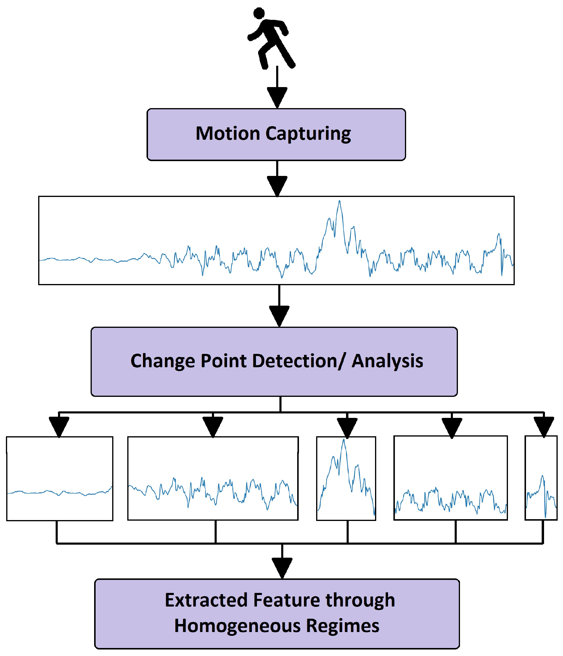
3.5. The Change Point Method

This is another assistant for the surrogate function to develop an interpretable model that can perfectly mimic the behavior of b. After globally approximating the model’s behavior in the previous subsection, our next task is feature discretization. In mathematics, discretization is the process of transforming a continuous variable to separate/distinct or non-continuous variables. This can be realized by converting analogue signals into digital signals in electrical engineering terms [67]. In machine learning vocabulary, discretization is to referred as partitioning or converting any continuous feature/attribute/variable in a dataset into nominal features. This process is an essential part of signal processing. Previously generated through the PDPBOX signal, this signal is to be processed in the following phase. However, there are different techniques and applications available for signal processing [68,69,70,71]; however, we considered the change point method technique for our task. According to [72], the change point technique is applicable to detect abrupt changes in any spatial data sequences. Change point analysis has evolved around detection analysis systems for applications such as those in human activity, environmental studies and quality control. [73] used the assistance of change point analysis in the underlying machine learning model’s signal or time series which was capable of detecting multiple change points in an underlying models’ behavior. The authors of [73] presented the ruptures Python library to perform offline and online multiple change point analysis. They elaborated a common workflow of change point detection in layman’s terms as the gait analysis shown in Figure 2.
The description of Figure 2 states that different motions—such as walking, sitting, running and jumping actions—performed by a human are monitored and captured through a device such as an accelerometer or gyroscope. The aim is to quantify gait characteristics [74,75]. The actions are recorded in the form of signals and then homogeneous patterns are analyzed. After analyzing homogeneous patterns, these patterns are broken down into different regimes for further feature extraction processing. Then, the resulting non-overlapping segments’ succession depicts the corresponding actions performed by a human as an object under test. Such an analysis therefore requires a prerequisite for signal processing such as the change point detection method. This method is categorized into two main branches: offline methods, which detects changes when all the data (samples) are received; and the online method, which aims to detect changes whenever they occur in real time. For our purposes, we considered the offline method.
Common notations are necessary to understand change point methodologies. For instance, we considered the fact that we have a non-stationary random process h = { h 1 h T } (in our case, these are generated from the PDPBOX estimator) with T samples—where h is piece-wise stationary signals. Abrupt change(s) in h occurred at instants t 1 * , t 2 * , t K * . Change point detection will assist us in finding the change(s) which occurred in t K * . Moreover, the number of changes K * that ’may or may not be known’ also need to be calculated, in function of the context we are dealing with. Change point detection is formally cast as model [73] (bottom–up segmentation, window-based methods, binary segmentation, etc.) selection seeking the best segmentation T in a given signal h through quantitative criterion [73]:
V = ( T , h )
Equation (8) has to be minimized [76]. Thus, the criterion function V = ( T ) for a particular segment can be denoted as
V = ( T , h ) : = K = 0 K c ( h t k h t k + 1 )
where c ( . ) is a cost function to measure the goodness-of-fit of a sub-signal h t k h t k + 1 . Here, we can write h t k h t k + 1 = { h t k + 1 t k + 1 } to a specific model because a given sub-signal can be written as h = { h t } t = 1 T and the complete signal is h = h 0 T for a specific model. Therefore, we can write the whole Equation (9) as
V = ( T , h ) : = c ( { h t } t 1 t 1 ) + c ( { h t } t 1 + 1 t 2 ) + c ( { h t } t 2 + 1 t 3 ) + c ( { h t } t i + 1 t i )
Moreover, the best segmentation T ^ is the minimizer V = ( T ) depending on the context, i.e., whether the number of change points K * is known. In our research work, the number of change points is unknown. Hence, the formula we will be following [73] is:
m i n T V ( T ) + p e n ( T )
In the above Equation (11), p e n ( T ) is the regularizer of partition T for ultimately creating stationary signals from non-stationary signals. The topology for change point detection works is mentioned in Figure 3.

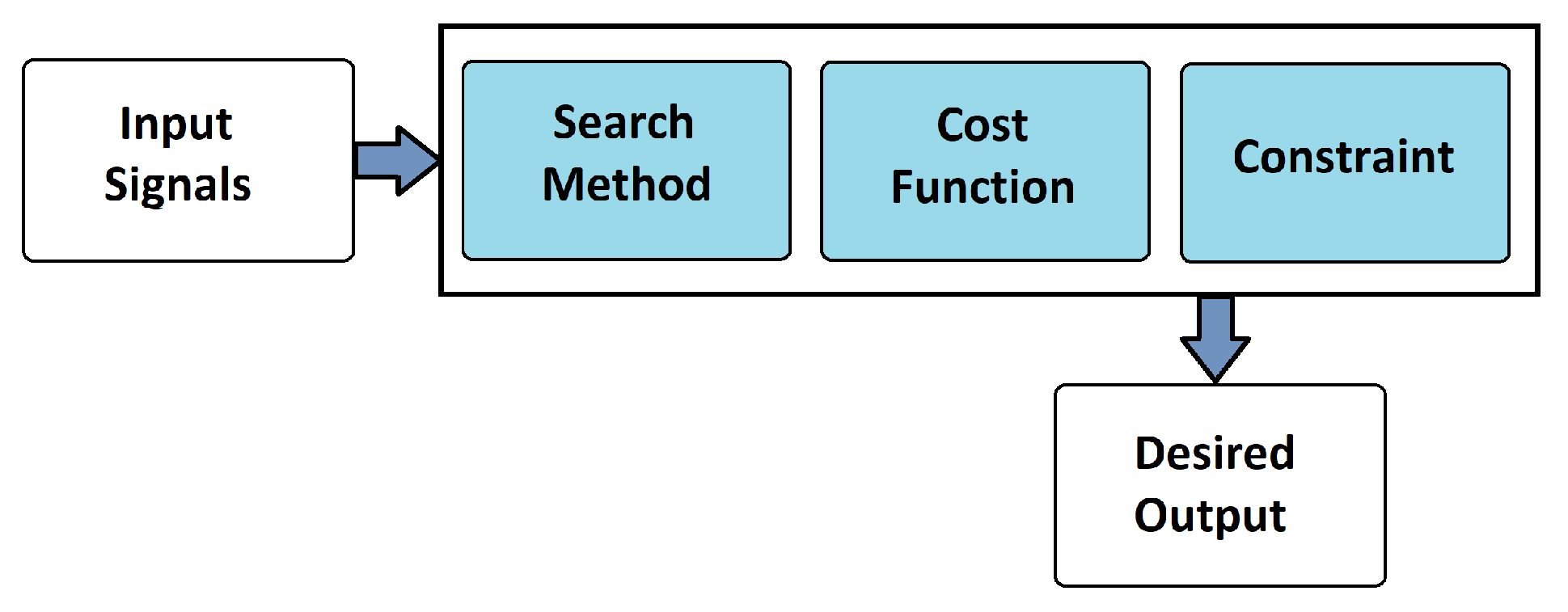
3.5.1. Cost Function

The cost function c ( . ) is the measure of homogeneity in a signal under investigation which depends on the choice of changes that must be detected. If c ( . ) is low, then the sub-signal h = { h t k + 1 t k + 1 } is homogeneous.

3.5.2. Search Method

There are several methods and algorithms available to solve the problem of the resolution procedure for the optimization of m i n T V ( T ) + p e n ( T ) ). These were chosen by developers based on a trade-off between accuracy and complexity. Nonetheless, numerous algorithms are available, e.g., dynamic programming, binary segmentation, and bottom-up segmentation, but for our research work, we will be focused on exact segmentation: the pruned exact linear time (PELT) [46] model. The reason behind using this problem solution is that it has the lowest computational cost and it is linear in nature, hence achieving the objective function which is minimizing the penalized sum of costs. Formally linear penalties [46] can be defined as
p e n ( T ) = ρ | T |
where ρ is the smoothing parameter. In our case, we will be dealing with linear penalties. Therefore, the pruning rule will work with the following concept in order to accelerate the process:
i f m i n V ( T , h 0 . . . t ) + ρ | T | + c ( h t . . . b ) m i n V ( T , h 0 . . . b ) + ρ | T |
If Equation (13) is satisfied, then t is not the last change point in the T set where t and b can be considered as two indexes ( t < b < T ) . A detailed algorithm is described in [77].

3.5.3. Constraint

By constraint is meant the constraint on the number of change points in an unknown problem Equation (11). It is necessary to add the complexity penalty p e n ( . ) in Equation (11) in order to balance out the goodness-of-fit for Equation (8). Note that the complexity penalty selection is dependent on the amplitude of changes. Thus, if penalization is too small, then many change points will be detected; conversely, much larger penalization will detect only significant ones. Hence, in our case, these change points will assist us in generating new features from the feature of the original dataset under investigation.
Note that, for this research work, we used a linear penalty for Equation (11) (also known as l 0 ) as referred to in [46]. More detail about this can be found under [73]. According to [46], the linear penalty l 0 is the most popular choice among developers because it generalizes the Bayesian information criterion (BIC) and the Akaike information criterion (AIC) (a stopping criterion splitting sub-signals in an iterative manner) [78,79].

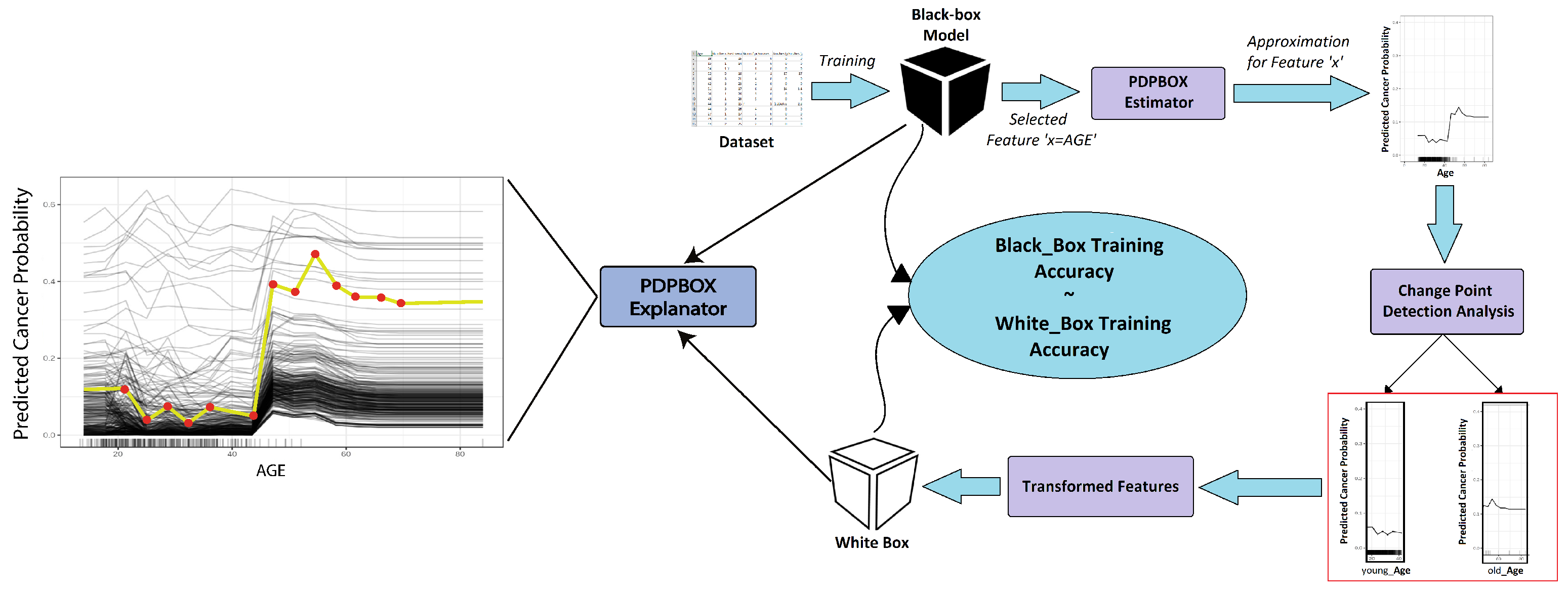
3.6. Enhanced Surrogate-Assisted Feature Engineering

In this sub-section, we map all the components that we discussed earlier in order to build ESAFE. ESAFE is a model agnostic which means it has the ability to accommodate any kind of black box as well as white box machine learning models, which means that the b and produced interpretable C g l o b a l (the end model for interpreting b) will be of any kind. We employed a surrogate model for feature engineering and to mimic the behavior of b. Before feature engineering, the partial dependence estimator facility provided by PDPBOX (discussed in Section 3.4) will produce grid points. In feature engineering, the feature space further expands from X to X * after being processed on recently generated grid points. This feature space X * is generated right after processing with the help of the change point detection technique which is discussed in detail in Section 3.5 of this section. Then, these newly generated features X * are transformed and exposed to any kind of white box model for training which will eventually produce C g l o b a l . Then, the produced C g l o b a l measurement is analyzed with some performance metrics. If the performance of C g l o b a l is approximately equal to or better than b, then we can say that our technique model is interpretable. Then, through C g l o b a l , we will produce the explanation ε g l o b a l with the PDPBOX graph. The surrogate model f is responsible to fit our data as best as possible. The accuracy of the black box model is directly proportional to the level of presentation of data. Therefore, we must be certain about the data we are feeding to achieve the maximum throughput of model that will be trained later on the glass box model to achieve best results. Now, referring to Equation (4), the surrogate function f contains the PDPBOX and change point detection technique which will accommodate b and input X. The PDPBOX will generate grid points and then, through those grid points, a new feature is generated with the help of change point detection. Note that we will be using continuous features for processing. The processing of categorical features is the same as that used in paper [44].
Figure 4 illustrates the inner working of the proposed solution used for continuous feature processing. The main components involved in processing continuous features are expressed in Figure 4.
In Figure 4, the input Dataset [80] is trained on a non-linear model (RF, GBR, etc.). The PDPBOX estimator will allow us to generate the behavior (by generating grid points in the form of signals) of the non-linear model’s prediction for each value of each feature x i ; then, through that, the change point detection component will assist us in detecting significant changes in the recently generated behavior which become signal(s) through the percentile points technique. This will separate the detected change points (based on homogeneous segments) in the form of newly generated features x * . Then, x * are allowed to train on the new white box (an interpretable) model. After measuring the accuracy of the white box model, we can conclude the primary interest which ensures that the prediction accuracy of b and the white box ( C g l o b a l ) models are as close as possible—if this is satisfied, then our goal is achieved. Note that the process from the PDPBOX estimator generation to the generation of newly generated features x * indicates automatic feature engineering and the process from accepting all predictions of black box b to the training of white box is contained in surrogate function f.
The proposed algorithm works in following fashion:
  • PDPBOX estimator approximates b’s behavior for selected feature(s) in the form of signals;
  • Then, the approximated signal is further processed for detecting multiple offline change points that are likely to appear in a generated signal;
  • Detected change points are then fitted with algorithms e.g., binary segmentation and exact segmentation for the creation of new regimes (features);
  • It is then transformed into a new dataset for a selected feature;
  • These transformed data are then trained on the white box model to achieve results close to black box model’s predictions.

3.7. Handling Algorithm’s Smoothing Parameter

As discussed with regard to the linear penalty in Section 3.5, we refer to Equation (11) p e n ( T ) which will define the number of possible segmentations in a non-stationary signal. If we excessively increase its value, then the window size for capturing significant changes in a given signal (produced by the PDPBOX estimator) will be lost. If we excessively decrease the value, then even minute changes in signals are detected which will eventually increase the complexity. This scenario will lead to the trade-off between goodness-of-fit and complexity. We denoted this parameter in upcoming section with λ . Thus, we manipulated the smoothing parameter λ with a predefined loop by setting some boundaries using the arithmetic progression formula:
t n a ( n 1 ) = d
In Equation (14), n is the total number of iterations, a is the starting point of iterations, where t n will be the last term and d will be the calculated steps, or it is the value given to the λ . When the iteration process is executed, then different values of λ will be generated and each of them will be fed to a training session so that the corresponding results generated after training and testing are recorded. Among the multiple values of λ corresponding to estimated results, the most accurate one is selected and base-lined.

3.8. Basic Workflow

Figure 5 illustrates the basic workflow of the proposed algorithm. The goal is to divide features in a dataset into new features which are categories and then transform those new feature values into subset they belonged to. In the form of a loop, the proposed technique will process each feature present in the original dataset. For each feature’s processing, this framework will check the nature of the feature, i.e., whether it is categorical or continuous. If the feature is continuous, then it will be passed to the PDPBOX estimator that will generate some behavioral pattern against the selected feature. The change point method will then detect abrupt changes in the generated behavior. Then, that feature x i is marked as processed. If the feature is categorical, then it will perform hierarchical clustering in order to group similar features into separate tree-like structures. Then, through the kneed locator algorithm [81], which approximates knee (elbows) points that are good enough to detect the maximum curvature, the tree height will be reduced whilst preserving the overall behavior of the prior surrogate model. Then, based on the biggest similarity in the response between categories, they are merged together to form new categories. New categories are generated and then trained on a white box model.
A detailed pseudo code of the algorithm is given in Appendix A and the computational complexity of the algorithm is discussed at Appendix B of this article.

4. Results and Benchmark

As far as the simulation is concerned, we tested our proposed extension on a machine with the following specifications: Intel Core [email protected] GHz processor; 12.0 GB of installed memory (RAM) with Microsoft Windows 10 Home operating system. We selected several datasets which are described in detail in subsequent subsections in order to deliver the validity of the proposed solution. For a lucid account, these datasets belong to classification and as well as regression problems. The package PDPBOX which assisted the ESAFE building comprehension for the black box model and estimated the model before change point detection during the processing of continues variable can be found at link https://github.com/SauceCat/PDPbox (accessed on 29 August 2021). The code that performs ESAFE with scikit-learn models [82] can be requested from any author of this work via respective emails. The SAFE ML code along with relevant examples is available at link https://github.com/ModelOriented/SAFE (accessed on 29 August 2021).

4.1. Regression—Boston Housing Dataset

We performed our technique on the Boston housing dataset [83]. This dataset was gathered by the United States Census Bureau on housing in the Boston, Massachusetts area. According to the authors, the sole purpose behind constructing such a dataset was to provide support to methodologies to measure the willingness of an individual to pay for clean air with the help of a housing price model, i.e., determining how much is more individuals are willing pay for a unit located in an excellent air quality location rather than another equivalent apartment located in a low air quality area to eventually allow quantitative estimations. This dataset comprises 14 columns wherein there are 13 independent variables and 1 dependent variable called the median value of owner-occupied homes as medv. The feature used in this dataset are described as follows: CRIM—per capita crime rate by town; ZN—proportion of residential land zoned for lots over 25,000 sq.ft; INDUS—proportion of non-retail business acres per town; CHAS—Charles River dummy variable (1 if tract bounds river, 0 otherwise; NOX—nitric oxides concentration (parts per 10 million); RM—average number of rooms per dwelling; AGE—proportion of owner-occupied units built prior to 1940; DIS—weighted distances to five Boston employment centers; RAD—index of accessibility to radial highways; TAX—full-value property-tax rate per USD 10,000; PTRATIO—pupil–teacher ratio by town; B 1000 ( B k 0.63 ) 2 where Bk is the proportion of African Americans by town; and LSTAT—% lower status of the population. After successful implementation with the help of the best value for regularizer penalty λ , we were able to achieve fine results that were higher in performance, computationally cheaper, and at the same time, transparent. A clear picture of the results is mentioned in Table 2.
Different machine learning models are compared in Table 2 with respect to the processing time and mean squared error (MSE). The lower the MSE of the model, the more accurate it will be. Moreover, we can see that the proposed extension’s MSE is close to the MSE of the surrogate model GBR (fidelity achieved). This was just a glimpse of the proposed solution. In forthcoming subsections, the sole purpose of the model and its capabilities are discussed in detail.

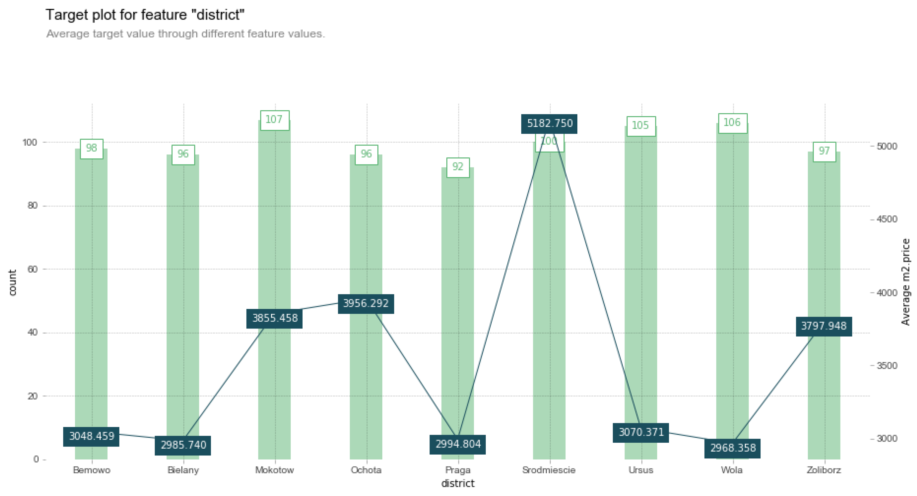
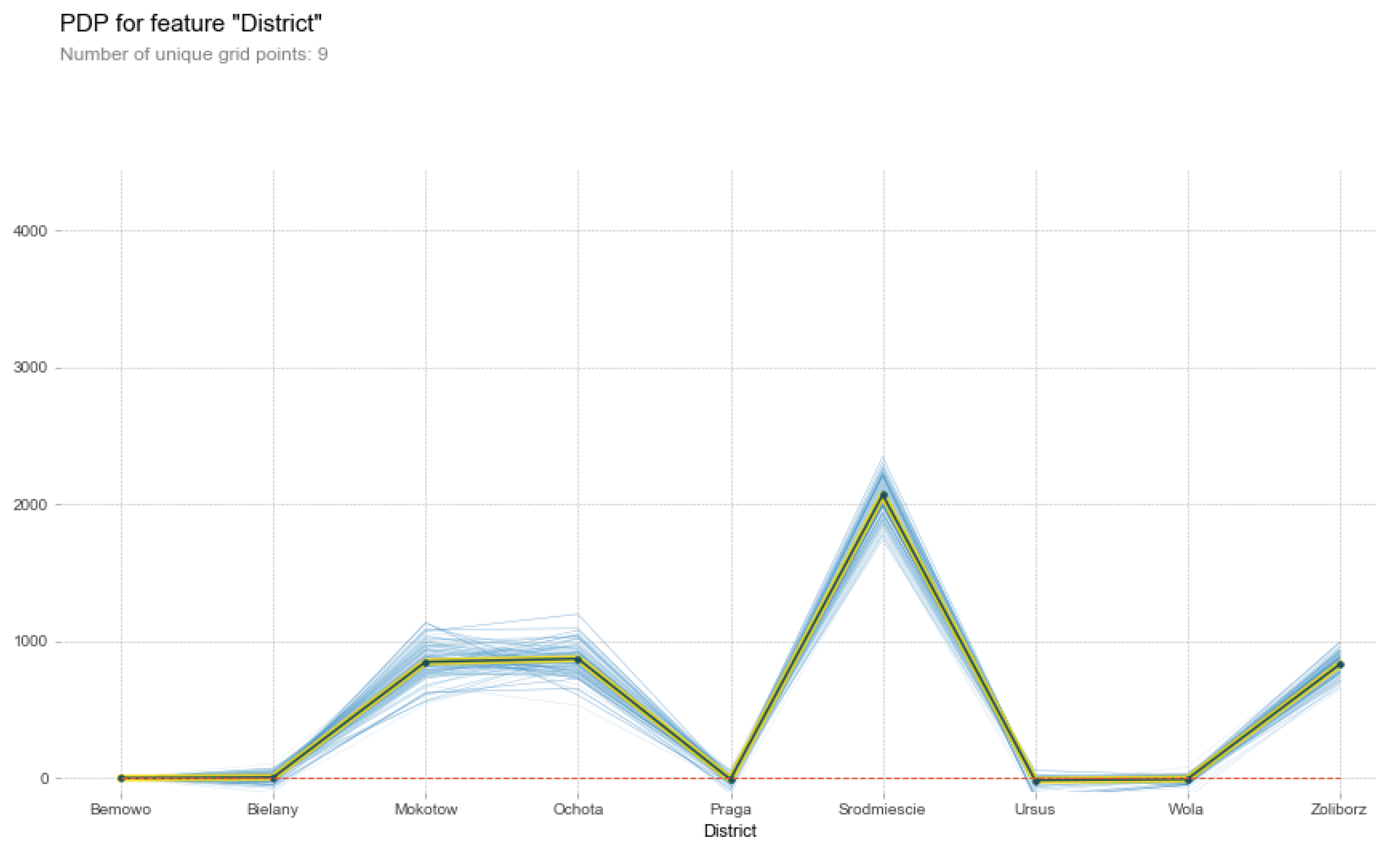
4.2. Regression—Warsaw Apartments Dataset

4.2.1. Data Information

This dataset is actually a subset of the dataset ‘Apartments’ [84] available at website https://www.oferty.net (accessed on 13 March 2021). which was introduced for predicting the individual price of houses located in Warsaw, Poland, on the basis of different factors that are the dataset’s independent variables. Those factors are ‘surface’, showing the area of the apartment in square meters; ‘district’, showing a factor corresponding to the district of Warsaw with the levels Mokotow, Srodmiescie, Wola and Zoliborz; ‘n.rooms’, representing the number of rooms per apartment; ‘floor’, showing the floor on which the apartment is located; ‘construction.date’, depicting the year that the apartment was constructed; and ‘areaPerMzloty’, showing the area in square meters per million zloty. This subset consists of six columns, as described earlier, including a target variable “price” and 1000 instances. ESAFE, in addition to other algorithms as competitors of ESAFE, are mentioned in Table 3 with respect to their respective performances.

4.2.2. Approximation and Manipulation

We began with the demonstration for approximating the black box b that is GBR. We tuned some different parameters of different algorithms mentioned in Table 3. For GBR, we set the number of estimators to 100 and the learning rate was set to 0.4 with a max depth = 4. Then, using Equation (14), we made an iteration where the processing of the best λ value was selected which was 4.17 . Then, the transformed features X * produced from the ruptures package (a part of the surrogate function f) were then trained on the interpretable model C g l o b a l ; in this case, we used linear regression (LR) as the interpretable model. Thus, in this particular example, for approximating how efficient our f is in imitating or performing better than b (fidelity), we again considered MSE. The R2 Score (performance measurement parameter) was also incorporated to ensure that the calculated MSE for each algorithm was not misleading. Thus, quantifying them through different dimensions is necessary. Such a deep analysis can also be applied to a previous problem domain (Boston housing) as well. The R2 Score is basically the proportion of variance in the dependent variable that is predictable from the independent variable(s). Thus, in other words, it can be defined as (total variance explained by model)/total variance. If the output of the R2 Score is 1 or 100%, then this means that there was no variance at all in underlying model during testing.
Table 3 depicts that what we desired was achieved. ESAFE performed better than GBR and LR but SAFE ML’s performance was little bit better than ESAFE. The reason for this is that we computed PDPBOX during the feature (numerical) transformation with the percentile method instead of considering every axis point generated from traditional PDP.

4.2.3. Explanation

For the explanation ε g l o b a l of previous measurements and calculations, we start from the target distribution which is how our target variable—the price per square meter m2·divided by the price of each apartment on different independent variables, e.g., surface and construction year—affect the overall prediction. Figure 6, a target plot, shows the target distribution for the independent numerical variable surface.
Figure 7 shows the distribution of data based on prediction that the underlying black box model b has made against a selected numeric feature surface. Similarly to Figure 6, Figure 7 also illustrates the same behavior but with a different angle in the form of curves. The y axis with the label (count) in Figure 6 represents the total number of houses for each surface area in square meters, categorized in different chunks as labeled in the x axis. The x axis, denoted as ’surface’ in the display column, defines the specified percentile range that is 10 in our case.The label average m2·price shows the average price against each unique grid and the negative signs with each unique value indicates the negative effects of each average value. Thus, the overall behavior constitutes the negative relation among the distributed values of the variables surface and m2·price. Small blue boxes that are connected through blue lines to other blue boxes are the average values of price in each percentile bucket.
The plot in Figure 7 shows the global (marginal) and local (each individual instance of) behavioral effect of the black box. In this explanation ε , we can see that each unique point is averaged with the help of the percentile = 10 (details are provided in [34]) which helps create points on the grid. The y axis label represents the prediction effects. From surface = 20 onward, the model begins to predict proceeding values with a negative relation. The blackish-yellow line represents the marginal effect of the prediction that GBR has made while the multiple thin blue lines show the effect of each instance on the target variable m2·price.
Thus, Figure 6 and Figure 7 seems incorrect, because both show behaviors that differ from that in a real-life world scenario. Common intellect does not accept the fact that the surface area of an apartment with a smaller value has a higher price. Therefore, some other variables are also required to investigate the matter. This will lead the user to explore hidden facts in a given dataset. Figure 8 unveils a hidden fact behind such a behavior against its distribution pattern.
We then generated another explanation ε which is represented in Figure 8, where the y axis with a label count represents the number of houses for each district. The x axis with the label district shows the districts of apartments dataset. The y axis on the right side labeled with the average m2· price shows the average price of houses in each percentile bucket. The Srodmiescie district with a total of 100 houses shows the highest average price which is PLN 5182.750 . On the other hand, the Wola district shows the lowest average price, i.e., PLN 2968.358 .
The distribution of data for the feature district depicts that the factor of the price of each apartment is also dependent on the district in which apartment is located in Warsaw, Poland. Similarly to the target distribution plot in Figure 8, Figure 9 also represents the same behavior with marginal as well as conditional effects of the district. The prediction distribution curves in Figure 9 for the variable district account for the fact that, on average, Srodmiescie has the highest price rates regardless of other variables.
As ICE curves, the blue lines in Figure 9 show the instance level explanation and the highlighted one represents the marginal distribution that explains the overall average effect of the feature district on the prices of apartments.
Interpretation, hence, prevents the generation of misleading information by exposing unprecedented factors and guides the user regarding how data are distributed through the original dataset and how a particular feature or features affect the prediction of the black box model b. If any changes are required in b, then through C g l o b a l , one can make changes because C g l o b a l is now our underlying model that captures all the behavior of b according to Equation (4)which was satisfied in the Approximation and Manipulation Section 4.2.2. With higher accuracy, the model is able to explain the behavior of the underlying b. This way, the purpose of trust is achieved.

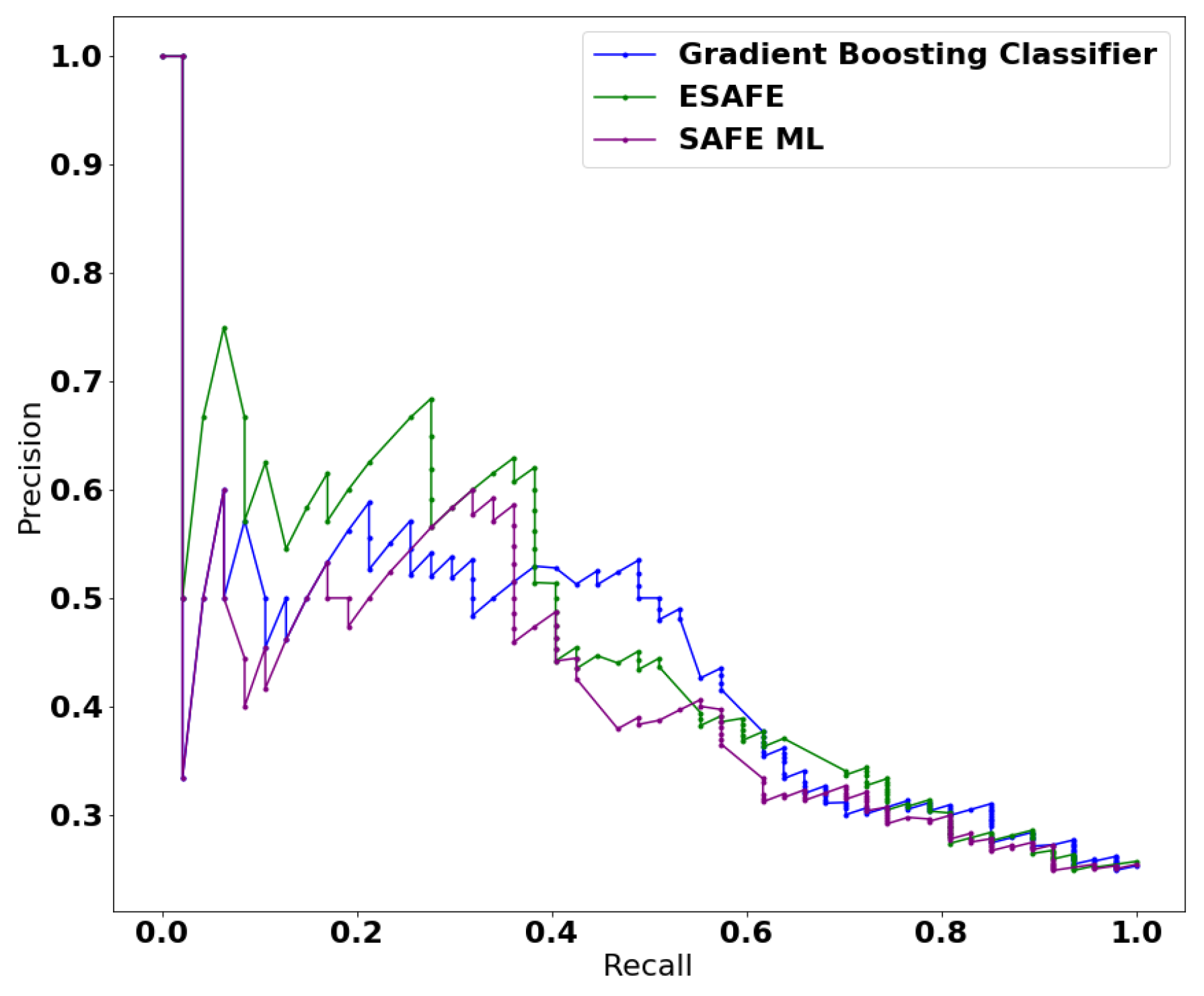
4.3. Classification—Blood Transfusion Dataset

4.3.1. Data Information

This dataset [85] was actually taken from the Blood Transfusion Service Centre in Hnsin Hsin-Chu City, Taiwan and represents a classification problem. The motivation behind the existence of such a dataset was to demonstrate an RFMTC marketing model allowing researchers to discover the knowledge of selecting targets from a database. The authors randomly selected 748 donors from the donor database. From those 748 donors’ data, each one included R (recency—months since last donation); F (frequency—total number of donations); M (monetary—total blood donated in c.c.); T (time—months since first donation); and a binary variable representing whether the subject donated blood in March 2007 in the form of 0 and 1 (1 indicating Yes and 0 meaning No). There are 5 columns and 748 rows in this -+dataset.

4.3.2. Approximation and Manipulation

As previously mentioned in Section 1, in order to validate the statement = that surrogate models mimic ( f i d e l i t y measure) the actual b as closely as possible under the constraint that ε g l o b a l is interpretable, we can compare performance metrics such as receiver operating characteristic (ROC) and AUC to satisfy Equation (4). Thus, continuing with previous statements, we trained different models on the given dataset to then measure the capacities of each model with respect to accuracy (ACC) and precision–recall (PR). ACC gives the number of correct predictions made by the model. While PR can be separately defined as the ratio of true positive instances that are actually positive, recall is the ratio of positive instances in which our model predicted correctly [86].
There is a separate debate about choosing specific performance metrics for classification problems [87]. Generally, PR is used in cases where the provided dataset is highly skewed (meaning a great difference between the distributed binary classes in the target variable) [88]. In this dataset (blood transfusion data), a binary classification problem is that of the imbalanced dataset. The target variable whether the subject donated blood in March 2007 in the form of 0 and 1, distributed as 1:178 and 0:570. Thus, we will use PR and ACC for performance measurement. Then, we will generate the area under the curve (AUC) which will summarize the totality of the area under the PR curve.
The PR curve for the gradient boosting classifier (GBC) algorithm was constructed by setting some optimal threshold such as the number of estimator, which were set to 500, and the learning rate was fixed to 0.11 . However, the ACC for the same GBC algorithm was higher— 75.40 % —but the estimated AUC was lower. The reason for this is that ACC was evaluated on a majority class with a higher population of true negatives in the given dataset. Meanwhile, the PR curve provides an entirely different interpretation of the result because it does not consider the true negative values (a population of people who did not donate blood in March 2007)—hence having no impact on true negatives. Figure 10 shows and compared different algorithms. The optimal parameter was picked from multiple iterations using the formula mentioned in Equation (14) with a = 0.1 , n = 25 and t n = 2, and then the optimal penalty selected from the iteration was λ = 1.02 . Both the SAFE ML’s and GBC’s curves overlapped when the curves crossed the R e c a l l value of 0.6 and from this point, SAFE ML started mimicking the GBC as b. On the other hand, ESAFE, which outperforms the SAFE ML when a = 0.1 , n = 25 and t n = 2, was defined from which λ = 1.3 was selected as the optimal parameter for producing the maximum AUC for this dataset. Figure 10 represents the one picture depicting all the involved algorithms performing the data transformation and making a prediction at the same time.
Table 4 summarizes the overall performances of different algorithms, wherein the proposed technique ESAFE outperforms the other algorithms. Thus, Figure 10 represents the whole inner workings while calculating the AUC-PR for each algorithm. In this sense, ESAFE covered the most area under the PR curve. The main reason for it having the lowest AUC is that these models predicted probabilities with uncertainty regarding some cases. These are exposed through the different thresholds evaluated in the construction of the curve, flipping some class 0 to class 1, offering slightly better precision but with very low recall. One important element which needs to be noted here is that the process time includes the iteration for finding the optimal penalty λ along with all the transformation of the feature space X while imitating b.
For the explanation ε g l o b a l part for C g l o b a l prediction, we sought to select the most important feature affecting our prediction; here, we chose the RF algorithm in order to identify the most important feature [89]. Among the four features with respect to the relevancy towards the target variable—which is whether the subject donated blood in March 2007—the feature time (months) was more important than any other feature in the dataset with 0.42 importance.

4.3.3. Explanation

We attempted to interpret the most important feature that the RF algorithm selected for us, which was time (months), as illustrated in Figure 11. In contrast to Figure 11, we also trained the same dataset on another b.
The middle line highlighted in Figure 11 shows a marginal effect of the feature time (months) on the prediction of whether the subject donated blood in March 2007. Negative values in the y-axis mean that the Yes/1 class has a negative relationship with the independent variable x axis. Similarly, positive values mean that the Yes/1 class has a positive relationship with the independent variable. Clearly, zero implies no average impact on the class probability according to the model. On the other hand, multiple thin blue lines represent the conditional effect of prediction on each instance.
Therefore, Figure 11 ensure that none of the information that b estimated is lost. As discussed in Section 1, this package will reflect the true meaning of being model agnostic, shown in the testimony describing how this dataset was also trained on the random forest classifier (RFC); this is explained through the PDPBOX explainer of how probability distributions are arranged throughout the dataset.
As we can see in Figure 12, a slightly changed behavior from Figure 11 occurred after the percentile (33.33, 44.44) curve began to change its direction towards percentile 88.89. The reason behind such a slight change in the curve was that the number of estimators in the RFC algorithm was different; moreover, the calculation of the algorithm was also different in nature.
The overall behaviors in both Figure 11 and Figure 12 are almost the same. We can conclude from the given problem discussed in detail that we satisfied Equation (4) by producing C g l o b a l and the explanation ε against a different bs.

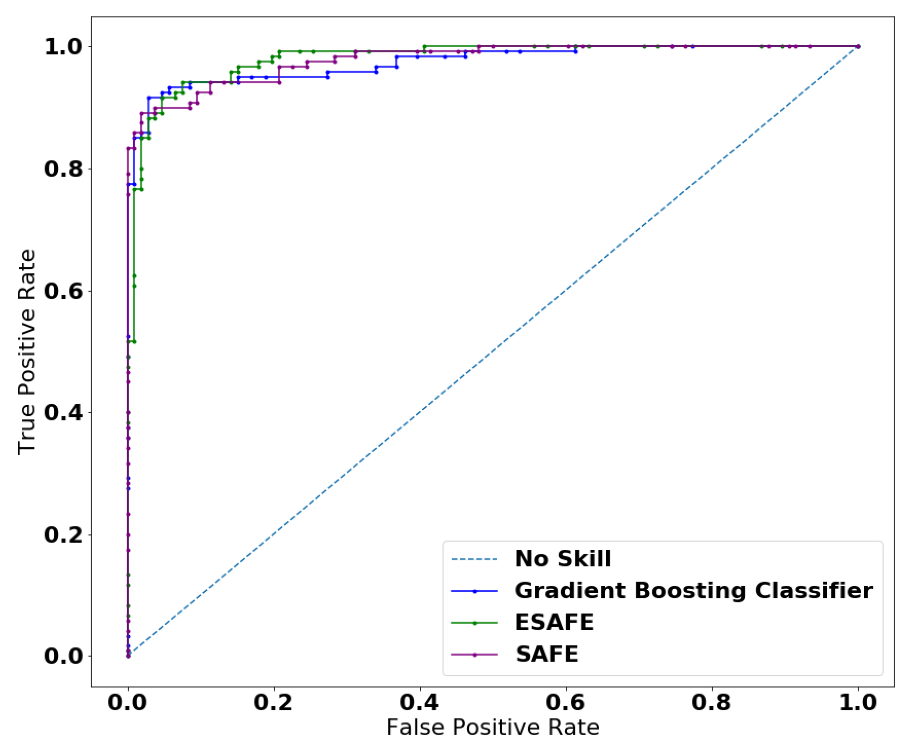
4.4. Classification—Student Performance Dataset

4.4.1. Data Information

This dataset was obtained from [90]. This dataset contains datasets from educational institution in both Iran and Portugal, but we selected the dataset for educational institutions in Portugal in which all the information is related to students’ achievement in secondary education at two Portuguese schools. This dataset contains 31 variables including the target variable G3 which is the final grade of the student in numeric form ranging from 0 to 20; there are a total 649 instances in this dataset; it can also be manipulated both as regression and as well as classification and it has no missing values so we do not need to worry about the imputation task in this dataset. In this article, we will regard this dataset as a classification problem (discussed in subsequent phases). It has a set of factors (independent variables) that affect the students’ overall performance. We designed a subset of this original dataset D O as was performed in [61]. This subset D S D O contains 19 attributes, namely HealthStatus; TravelTimetoSchool; FamilyQualityLife; GoingOutWithFriends; Absence; sizeOfFamily; Mothers Job; Fathers Job; ExtraEducationalSupport; InternetAccess; romanticRelationship; Mother’sEducation; Father’sEducation; Parent’sStatus; theGoalPursuingEducation; FreeTimeAfterSchool; G1; G2; and G3.

4.4.2. Approximation and Manipulation

The target variable G 3 was converted into binary distribution so that if G 3 ≥ 10, then the student’s result will be marked as Passed (1)—or else marked as Failed (0). In a previous subsection of this article, evaluation was performed without balancing data which is another challenging task for developers. This dataset has an imbalanced target variable with distribution {1: 452, 0: 197}, which thus affects the accuracy metrics in such case. However, there are other performance metrics available but if the dataset is balanced, we can use the receiver operating characteristic (ROC) curves instead of PR curves for measuring the performance of algorithms. AUC, which is essentially the whole area under the ROC curve which is the relationship between the true positive rate and the false positive rate, represents a great tool for predicting the performance of a binary classifier. There are multiple performance metrics available for us such as F measure and ROC [91,92]. Generally, ROC is used when the given dataset is balanced. It is important to note that most of machine learning models work accurately when the given dataset is balanced by default; however, when it comes to skewed datasets, the results are entirely unpredictable [93]. For this dataset, we used an oversampling approach as if the given dataset is small, then an oversampling approach is the best feasible method—otherwise, for data that contain millions of tuples, then under-sampling is the best choice. To handle the given problem, we used the synthetic minority oversampling technique (SMOTE) [94]. Basically, this method is a technique that usually increases the number of minority class samples in a given dataset by generating new instances and these new instances are not copies of existing minority samples.
According to [86], using an ROC curve with an imbalanced dataset might be deceptive (providing an optimistic picture) and lead to incorrect interpretations of the model’s accuracy. The main reason for this optimistic picture of ROC is because of the use of true negatives in the false positive rate of the ROC curve and the careful avoidance of this rate in the PR curve. A whole summary of the comparison between different algorithms is given in Table 5.
Table 5 represents the case of this dataset in which, after balancing, all models are working perfectly with higher probabilities of guessing right answers. There are minute differences between each model’s performance on the data we provided. The AUC-ROC in case of LOR performs better than for GBC and SAFE ML. The reason for this is that the provided dataset has fewer instances with a large number of attributes so a monotonic (linear model) algorithm performed better in this regard [95]. Moreover, if we see that the process of the SAFE ML’s execution time includes the iteration time for finding the optimal parameter λ and transforming the feature space X into X * whilst simultaneously imitating GBC as b, this will produce C g l o b a l for further proceedings (ready for explanation through ε g l o b a l ).
The blue lines in Figure 13 represent no skill, which is basically a reference to all models with some skills, representing at which point the model’s skill has the largest distance from this no skill line (blue dotted lines). The ROC function in Python will access both true outcomes that are positive and will predict the probability for positive classes from the test set. The ROC will then return false positive rates for each threshold and a true positive threshold. The GBC’s result is shown in Figure 13 in which the AUC-ROC is measured with 0.975 as the highest prediction probability for true positive rates which depicts the higher performance of the model’s skill. This result was achieved by tuning parameters in the following fashion (number of estimators = 500 and learning rate = 0.15 ). In Figure 13, the models SAFE ML and GBC performed excellently and SAFE ML almost accurately mimicked GBC, whilst we set the main smoothing parameters with the help of same arithmetic progression iteration with the following boundaries a = 0.01 , n = 20 and t n = 2. Here, the optimal parameter λ = 0.9 was selected. Then, ESAFE was introduced and compared with SAFE ML and GBC. All algorithms performed well with almost the same results but if we take a look at Table 5, ESAFE was far more efficient in estimating C g l o b a l . It took almost half an hour for SAFE ML to perform the same task. The optimal penalty λ = 0.011 —this will set the window size for estimating minute changes t K * in signal h from that same arithmetic progression formula using boundaries which are the same as those chosen for SAFE ML in this example. Then, in Figure 13, accumulative results are presented, from which anyone can interpret the performance of different models but ESAFE performs slightly better than SAFE ML.
Henceforth, this way we are able to produce C g l o b a l at the end where we imitated b through an interpretable model C g l o b a l using the process function f which helped in transforming and generating new features against each feature of the original dataset. Then, these new features were trained on LOR, also known as white box, which in our case is C g l o b a l . Figure 13 and Table 5 provide evidence that we produced the results through approximating C g l o b a l .

4.4.3. Explanation

For the explanation part ε g l o b a l of this example, we again employed the available feature importance technique [44] to detect which feature in the given dataset had the most important effect on the overall prediction of model b. Feature G 2 was the most important with a 0.87 importance rate. Thus, the PDPBox package again provides a lucid explanation of the average behavior produced from C g l o b a l as well as the instance-level behavior of model b under consideration for the selected feature. Figure 14 shows a clear explanation of the model’s behavior against the feature G 2 .
According to Figure 14, we can note that the target variable response abruptly changes after the percentile (22.22 to 44.44); and the average curve begins to change its direction but shows constant behavior after the percentile bucket (55.56). The overall picture can be interpreting as the number of passed students is higher. There is no negative relationship in the given feature as it starts from 0 which means there is no average impact on class probability. Hence, Equation (4) is once again satisfied by producing explanation ε and constructing C g l o b a l .
Similarly, for further interrogation, we may choose other features of the dataset to more precisely mimic the model’s behavior. Until now, we covered three main problem domains related to both classification and regression which were the Boston housing, Warsaw apartments and blood transfusion datasets. We can also treat other problems with our proposed solution such as yacht hydrodynamics from the UCI Machine Learning Repository [96] or real estate [97] which belong to the regression category; as well as Titanic from Kaggle [98], Pima Indian diabetes and risk factors for cervical cancer [80] which correspond to the classification domain.

5. Conclusions and Future Extension

In this research paper, we presented ESAFE (an extension of SAFE ML) and used a surrogate model that was capable of mimicking any black box model with a simple white box model. Evidence of ESAFE’s capabilities was provided in the form of benchmarking in Section 4 by considering different domains from different sources. As discussed regarding focal points in the introductory part, through the proposed technique, we gained higher fidelity, as measured in performance metrics, higher accuracy, and achieved comprehensibility after producing explanation. By virtue of ESAFE, one can rely on a machine without any doubt. ESAFE hereby provides a vital function for developers by easing the task of feature engineering during black box model approximation (imitation). Moreover, since it model agnostic, developers can employ any type of white box model. For the black box model, ESAFE sustains its quality of being model independent; thus, it accommodates any black box model as well. In addition to its multifaceted solutions, accuracy is maintained with cheaper computational power for making estimations (accuracy close to the accuracy of black box model). From an explanation point of view, we employed the same PDPBOX which will generate a graphical explanation for the end-user, meaning that with the same Algorithm, we can estimate and explain black box models. After receiving the explanation, an individual can comprehend which specific feature affects the overall black box model in which way/direction, which eventually allows the user to explore more features and their effects on predictions as elaborated in Section 4.2.3. This means that one can gain insights into other hidden patterns present in a given dataset. Thus, when a noisy datum is fed and a model behaves accordingly, the explanation would eventually expose the culprits responsible. From a subjective point of view, such a technique is not capable of acknowledging multiple classification problems. However, the technique is capable of producing C g l o b a l at a global level, so there is a need to have interpretation at an instance level; thus, we considered it as a future extension to make it interpretable at the local level as well. Therefore, in the future, we are expecting to add further functionalities as has been done for LIME [24]. This way, our technique will be interpretable at the global and local levels.

Author Contributions

The research conceptualization and methodology were performed by M.A., Z.A. and K.R. The technical and theoretical framework were prepared by A.M.K. and B.H. The technical review and improvement were performed by Z.P., M.I., K.R. and K.-I.K. The overall technical support, guidance and project administration were provided by B.H., T.-E.S., K.-I.K. and A.M.K. All authors have read and agreed to the published version of the manuscript.

Funding

This research received no external funding.

Acknowledgments

This work was supported by the Institute for Information & Communications Technology Planning & Evaluation (IITP) grant funded by the Korea government (MSIT) (No. 2019-0-01343, Training Key Talents in Industrial Convergence Security).

Conflicts of Interest

The authors declare no conflict of interest.

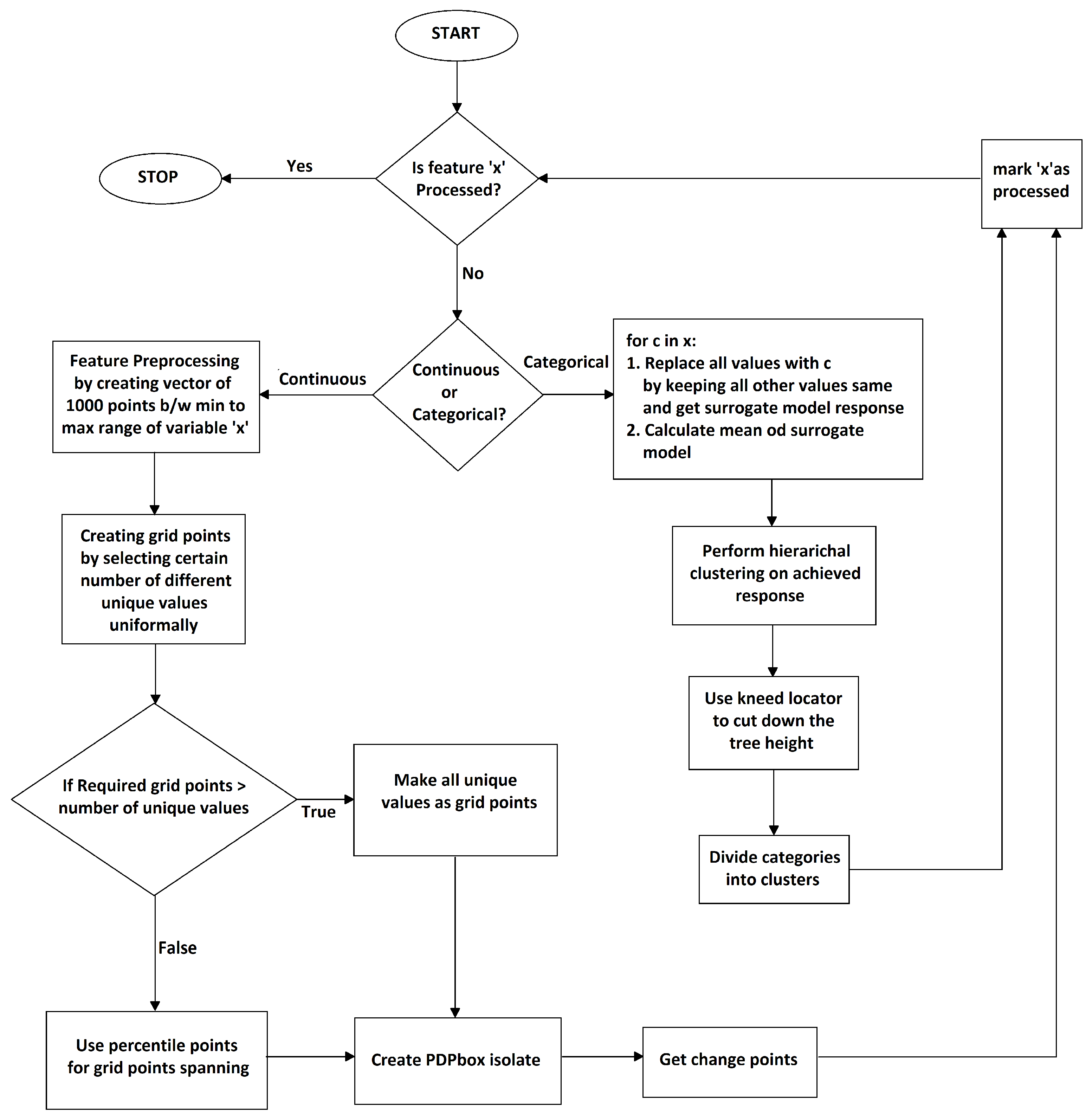
Appendix A. Algorithm for Proposed Extension ESAFE

Algorithm A1 Feature Engineering.
  •    for i = 1 to n do
  •       if  x i is Continuous then
  •             Parameters initialization for penalty ( P ), cost function ( l 2 ) and regularization (˘)
  •             Calculating PDPBOX
  •             if Model ( M ) is fitted then
  •                create array of input percentiles range æ
  •                æ must be (tuple And !( 0 > and < 100))
  •                calculate array of grid points(fi)
  •                if fi is type of æ then
  •                    assign grid_df = dataframe of dataset
  •                    for each i in grid_df do
  •                          i = percentile_grids
  •                          group them by values of grids
  •                    end for
  •                end if
  •             end if
  •             for j in feature grids do
  •                contact grid result saved in percentile information
  •             end for
  •             Fit the information previously fetched to rupture PELT search method
  •             Predict possible change points from fitted PELT method with l 2 model
  •             Save the new discretized information to x i *
  •       end if
  •       if  x i is Categorical then
  •             Calculate model response for each observation with imputed each possible value of x i
  •             Merge similar responses with the help of hierarchical clustering with clusters ˘ and form tree
  •             Use Kneed_Locator algorithm to cut down the height of trees and assign these newly created points on the basis of knees detected to transformation t i ( x ) that has converted x i to x i *
  •             Save the transformation with x i * as new dataset K n m
  •       end if
  •    end for
  •    Input: K ^ n m estimated from surrogate model M to new simple model M ^
  •    Fit M ^
  •    Predict the accuracy for M ^

Appendix B. Algorithm Complexity

For the discussion of the complexity measurement, we considered the time complexity of the proposed technique in a big (O) notation. The proposed algorithm has two scenarios upon which its time complexity varies. If the given dataset has both continuous and categorical variables, then the time complexity will be O( n 3 ) because an additional iteration will be required to deal with the categorical features in order to successfully convert them into continuous variables. If the dataset only contains continuous variables, then the time complexity will be O( n 2 ).

References

  1. Mullainathan, S.; Spiess, J. Machine learning: An applied econometric approach. J. Econ. Perspect. 2017, 31, 87–106. [Google Scholar] [CrossRef] [Green Version]
  2. Mohammadi, M.; Yazdani, S.; Khanmohammadi, M.H.; Maham, K. Financial Reporting Fraud Detection: An Analysis of Data Mining Algorithms. Int. J. Financ. Manag. Account. 2020, 4, 1–12. [Google Scholar]
  3. Awoyemi, J.O.; Adetunmbi, A.O.; Oluwadare, S.A. Credit card fraud detection using machine learning techniques: A comparative analysis. In Proceedings of the 2017 International Conference on Computing Networking and Informatics (ICCNI), Lagos, Nigeria, 29–31 October 2017; pp. 1–9. [Google Scholar]
  4. Raghavan, P.; Gayar, N.E. Fraud Detection using Machine Learning and Deep Learning. In Proceedings of the 2019 International Conference on Computational Intelligence and Knowledge Economy (ICCIKE), Dubai, United Arab Emirates, 11–12 December 2019; pp. 334–339. [Google Scholar]
  5. Sidiropoulos, N.D.; De Lathauwer, L.; Fu, X.; Huang, K.; Papalexakis, E.E.; Faloutsos, C. Tensor decomposition for signal processing and machine learning. IEEE Trans. Signal Process. 2017, 65, 3551–3582. [Google Scholar] [CrossRef]
  6. Paulus, M.T. Algorithm for explicit solution to the three parameter linear change-point regression model. Sci. Technol. Built Environ. 2017, 23, 1026–1035. [Google Scholar] [CrossRef]
  7. Rudin, C. Stop explaining black box machine learning models for high stakes decisions and use interpretable models instead. Nat. Mach. Intell. 2019, 1, 206–215. [Google Scholar] [CrossRef] [Green Version]
  8. Miller, T. Explanation in artificial intelligence: Insights from the social sciences. Artif. Intell. 2019, 267, 1–38. [Google Scholar] [CrossRef]
  9. Kim, B.; Khanna, R.; Koyejo, O.O. Examples are not enough, learn to criticize! criticism for interpretability. In Proceedings of the 2016 Advances in Neural Information Processing Systems, Barcelona, Spain, 5–10 December 2016; pp. 2280–2288. [Google Scholar]
  10. Azodi, C.B.; Tang, J.; Shiu, S.H. Opening the Black Box: Interpretable Machine Learning for Geneticists. Trends Genet. 2020, 36, 442–455. [Google Scholar] [CrossRef] [PubMed]
  11. Breiman, L. Random forests. Mach. Learn. 2001, 45, 5–32. [Google Scholar] [CrossRef] [Green Version]
  12. Cortes, C.; Vapnik, V. Support-vector networks. Mach. Learn. 1995, 20, 273–297. [Google Scholar] [CrossRef]
  13. Friedman, J.H. Stochastic gradient boosting. Comput. Stat. Data Anal. 2002, 38, 367–378. [Google Scholar] [CrossRef]
  14. Hinton, G.E.; Salakhutdinov, R.R. Reducing the dimensionality of data with neural networks. Science 2006, 313, 504–507. [Google Scholar] [CrossRef] [Green Version]
  15. Hinton, G.E.; Osindero, S.; Teh, Y.W. A fast learning algorithm for deep belief nets. Neural Comput. 2006, 18, 1527–1554. [Google Scholar] [CrossRef]
  16. Guidotti, R.; Monreale, A.; Ruggieri, S.; Turini, F.; Giannotti, F.; Pedreschi, D. A survey of methods for explaining black box models. ACM Comput. Surv. (CSUR) 2018, 51, 1–42. [Google Scholar] [CrossRef] [Green Version]
  17. Quinlan, J.R. Induction of decision trees. Mach. Learn. 1986, 1, 81–106. [Google Scholar] [CrossRef] [Green Version]
  18. Hastie, T.; Tibshirani, R.; Friedman, J. The Elements of Statistical Learning: Data Mining, Inference, and Prediction; Springer Science & Business Media: New York, NY, USA, 2009. [Google Scholar]
  19. Shah, A.; Lynch, S.; Niemeijer, M.; Amelon, R.; Clarida, W.; Folk, J.; Russell, S.; Wu, X.; Abràmoff, M.D. Susceptibility to misdiagnosis of adversarial images by deep learning based retinal image analysis algorithms. In Proceedings of the 2018 IEEE 15th International Symposium on Biomedical Imaging (ISBI 2018), Washington, DC, USA, 4–7 April 2018; pp. 1454–1457. [Google Scholar]
  20. Kroll, J.A.; Barocas, S.; Felten, E.W.; Reidenberg, J.R.; Robinson, D.G.; Yu, H. Accountable algorithms. Univ. Pa. Law Rev. 2016, 165, 633. [Google Scholar]
  21. Danks, D.; London, A.J. Regulating autonomous systems: Beyond standards. IEEE Intell. Syst. 2017, 32, 88–91. [Google Scholar] [CrossRef]
  22. Kingston, J.K. Artificial intelligence and legal liability. arXiv 2018, arXiv:1802.07782. [Google Scholar]
  23. Messalas, A.; Kanellopoulos, Y.; Makris, C. Model-Agnostic Interpretability with Shapley Values. In Proceedings of the 2019 10th International Conference on Information, Intelligence, Systems and Applications (IISA), Patras, Greece, 15–17 July 2019; pp. 1–7. [Google Scholar]
  24. Ribeiro, M.T.; Singh, S.; Guestrin, C. “Why should i trust you?” Explaining the predictions of any classifier. In Proceedings of the 22nd ACM SIGKDD International Conference on Knowledge Discovery and Data Mining, San Francisco, CA, USA, 13–17 August 2016; pp. 1135–1144. [Google Scholar]
  25. Johansson, U.; Sönströd, C.; Norinder, U.; Boström, H. Trade-off between accuracy and interpretability for predictive in silico modeling. Future Med. Chem. 2011, 3, 647–663. [Google Scholar] [CrossRef]
  26. Wang, T. Hybrid Decision Making: When Interpretable Models Collaborate With Black-Box Models. arXiv 2018, arXiv:1802.04346. Available online: https://arxiv.org/pdf/1802.04346v1.pdf (accessed on 29 August 2021).
  27. Hu, L.; Chen, J.; Nair, V.N.; Sudjianto, A. Locally interpretable models and effects based on supervised partitioning (LIME-SUP). arXiv 2018, arXiv:1806.00663. [Google Scholar]
  28. Stiglic, G.; Kocbek, P.; Fijacko, N.; Zitnik, M.; Verbert, K.; Cilar, L. Interpretability of machine learning based prediction models in healthcare. arXiv 2020, arXiv:2002.08596. [Google Scholar] [CrossRef]
  29. Lakkaraju, H.; Kamar, E.; Caruana, R.; Leskovec, J. Interpretable & Explorable Approximations of Black Box Models. arXiv 2017, arXiv:1707.01154. [Google Scholar]
  30. Ming, L.; Chao, Y. Mathematical Model and Quantitative Research Method on the Variability of Task Execution-time. In Proceedings of the 2012 International Conference on Computer Distributed Control and Intelligent Environmental Monitoring, Zhangjiajie, China, 5–6 March 2012; pp. 397–402. [Google Scholar]
  31. Justus, D.; Brennan, J.; Bonner, S.; McGough, A.S. Predicting the Computational Cost of Deep Learning Models. In Proceedings of the 2018 IEEE International Conference on Big Data (Big Data), Seattle, WA, USA, 10–13 December 2018; pp. 3873–3882. [Google Scholar]
  32. Tunstall, S.L. Models as Weapons: Review of Weapons of Math Destruction: How Big Data Increases Inequality and Threatens Democracy by Cathy O’Neil (2016). Numeracy 2018, 11, 10. [Google Scholar] [CrossRef] [Green Version]
  33. Gosiewska, A.; Gacek, A.; Lubon, P.; Biecek, P. SAFE ML: Surrogate Assisted Feature Extraction for Model Learning. arXiv 2019, arXiv:1902.11035. [Google Scholar]
  34. Goldstein, A.; Kapelner, A.; Bleich, J.; Pitkin, E. Peeking inside the black box: Visualizing statistical learning with plots of individual conditional expectation. J. Comput. Graph. Stat. 2015, 24, 44–65. [Google Scholar] [CrossRef]
  35. Zhou, Y.; Hooker, G. Interpreting models via single tree approximation. arXiv 2016, arXiv:1610.09036. [Google Scholar]
  36. Gibbons, R.D.; Hooker, G.; Finkelman, M.D.; Weiss, D.J.; Pilkonis, P.A.; Frank, E.; Moore, T.; Kupfer, D.J. The CAD-MDD: A computerized adaptive diagnostic screening tool for depression. J. Clin. Psychiatry 2013, 74, 669. [Google Scholar] [CrossRef] [Green Version]
  37. Tolomei, G.; Silvestri, F.; Haines, A.; Lalmas, M. Interpretable predictions of tree-based ensembles via actionable feature tweaking. In Proceedings of the 23rd ACM SIGKDD International Conference on Knowledge Discovery and Data Mining, Halifax, NS, Canada, 13–17 August 2017; pp. 465–474. [Google Scholar]
  38. Krishnan, S.; Wu, E. Palm: Machine learning explanations for iterative debugging. In Proceedings of the 2nd Workshop on Human-In-the-Loop Data Analytics, Chicago, IL, USA, 14–19 May 2017; pp. 1–6. [Google Scholar]
  39. Hara, S.; Hayashi, K. Making tree ensembles interpretable. arXiv 2016, arXiv:1606.05390. [Google Scholar]
  40. Cui, Z.; Chen, W.; He, Y.; Chen, Y. Optimal action extraction for random forests and boosted trees. In Proceedings of the 21th ACM SIGKDD International Conference on Knowledge Discovery and Data Mining, Sydney, NSW, Australia, 10–13 August 2015; pp. 179–188. [Google Scholar]
  41. Tan, P.N.; Steinbach, M.; Kumar, V. Introduction to Data Mining; Pearson Education Inc.: New Delhi, India, 2006. [Google Scholar]
  42. Tsanas, A.; Xifara, A. Accurate quantitative estimation of energy performance of residential buildings using statistical machine learning tools. Energy Build. 2012, 49, 560–567. [Google Scholar] [CrossRef]
  43. Collaris, D.; van Wijk, J.J. ExplainExplore: Visual Exploration of Machine Learning Explanations. In Proceedings of the 2020 IEEE Pacific Visualization Symposium (PacificVis), Tianjin, China, 3–5 June 2020; pp. 26–35. [Google Scholar]
  44. Friedman, J.H. Greedy function approximation: A gradient boosting machine. Ann. Stat. 2001, 29, 1189–1232. [Google Scholar] [CrossRef]
  45. Natekin, A.; Knoll, A. Gradient boosting machines, a tutorial. Front. Neurorobotics 2013, 7, 21. [Google Scholar] [CrossRef] [Green Version]
  46. Killick, R.; Fearnhead, P.; Eckley, I.A. Optimal detection of changepoints with a linear computational cost. J. Am. Stat. Assoc. 2012, 107, 1590–1598. [Google Scholar] [CrossRef]
  47. Vidovic, M.M.C.; Gornitz, N.; Muller, K.R.; Kloft, M. Feature importance measure for non-linear learning algorithms. arXiv 2016, arXiv:1611.07567. [Google Scholar]
  48. Sonnenburg, S.; Zien, A.; Philips, P.; Rätsch, G. POIMs: Positional oligomer importance matrices—Understanding support vector machine-based signal detectors. Bioinformatics 2008, 24, i6–i14. [Google Scholar] [CrossRef] [Green Version]
  49. Zien, A.; Krämer, N.; Sonnenburg, S.; Rätsch, G. The feature importance ranking measure. In Joint European Conference on Machine Learning and Knowledge Discovery in Databases; Springer: Berlin/Heidelberg, Germany, 2009; pp. 694–709. [Google Scholar]
  50. Montavon, G.; Lapuschkin, S.; Binder, A.; Samek, W.; Müller, K.R. Explaining nonlinear classification decisions with deep taylor decomposition. Pattern Recognit. 2017, 65, 211–222. [Google Scholar] [CrossRef]
  51. Sturm, I.; Lapuschkin, S.; Samek, W.; Müller, K.R. Interpretable deep neural networks for single-trial EEG classification. J. Neurosci. Methods 2016, 274, 141–145. [Google Scholar] [CrossRef] [Green Version]
  52. Guidotti, R.; Monreale, A.; Ruggieri, S.; Pedreschi, D.; Turini, F.; Giannotti, F. Local rule-based explanations of black box decision systems. arXiv 2018, arXiv:1805.10820. [Google Scholar]
  53. Freitas, A.A. Comprehensible classification models: A position paper. ACM SIGKDD Explor. Newsl. 2014, 15, 1–10. [Google Scholar] [CrossRef]
  54. Martens, D.; Vanthienen, J.; Verbeke, W.; Baesens, B. Performance of classification models from a user perspective. Decis. Support Syst. 2011, 51, 782–793. [Google Scholar] [CrossRef]
  55. Pazzani, M.J.; Mani, S.; Shankle, W.R. Acceptance of rules generated by machine learning among medical experts. Methods Inf. Med. 2001, 40, 380–385. [Google Scholar]
  56. Verbeke, W.; Martens, D.; Mues, C.; Baesens, B. Building comprehensible customer churn prediction models with advanced rule induction techniques. Expert Syst. Appl. 2011, 38, 2354–2364. [Google Scholar] [CrossRef]
  57. Ustun, B.; Rudin, C. Supersparse linear integer models for optimized medical scoring systems. Mach. Learn. 2016, 102, 349–391. [Google Scholar] [CrossRef]
  58. Ahmad, M.A.; Eckert, C.; Teredesai, A. Interpretable machine learning in healthcare. In Proceedings of the 2018 ACM International Conference on Bioinformatics, Computational Biology, and Health Informatics, Washington, DC, USA, 29 August–1 September 2018; pp. 559–560. [Google Scholar]
  59. Kotthoff, L.; Thornton, C.; Hoos, H.H.; Hutter, F.; Leyton-Brown, K. Auto-WEKA 2.0: Automatic model selection and hyperparameter optimization in WEKA. J. Mach. Learn. Res. 2017, 18, 826–830. [Google Scholar]
  60. Jin, H.; Song, Q.; Hu, X. Auto-Keras: An Efficient Neural Architecture Search System. In Proceedings of the KDD ’19: 25th ACM SIGKDD International Conference on Knowledge Discovery & Data Mining, Anchorage, AK, USA, 4–8 August 2019; Association for Computing Machinery: New York, NY, USA, 2019; pp. 1946–1956. [Google Scholar] [CrossRef] [Green Version]
  61. Ghorbani, R.; Ghousi, R. Comparing Different Resampling Methods in Predicting Students’ Performance Using Machine Learning Techniques. IEEE Access 2020, 8, 67899–67911. [Google Scholar] [CrossRef]
  62. Khurana, U.; Turaga, D.; Samulowitz, H.; Parthasrathy, S. Cognito: Automated Feature Engineering for Supervised Learning. In Proceedings of the 2016 IEEE 16th International Conference on Data Mining Workshops (ICDMW), Barcelona, Spain, 12–15 December 2016; pp. 1304–1307. [Google Scholar]
  63. Bahnsen, A.C.; Aouada, D.; Stojanovic, A.; Ottersten, B. Feature engineering strategies for credit card fraud detection. Expert Syst. Appl. 2016, 51, 134–142. [Google Scholar] [CrossRef]
  64. Hocking, R.R. A Biometrics invited paper. The analysis and selection of variables in linear regression. Biometrics 1976, 32, 1–49. [Google Scholar] [CrossRef]
  65. Ribeiro, M.T.; Singh, S.; Guestrin, C. Model-agnostic interpretability of machine learning. arXiv 2016, arXiv:1606.05386. [Google Scholar]
  66. Greenwell, B.M. pdp: An R package for constructing partial dependence plots. R J. 2017, 9, 421–436. [Google Scholar] [CrossRef] [Green Version]
  67. Bashir, S.; Ali, S.; Ahmed, S.; Kakkar, V. Analog-to-digital converters: A comparative study and performance analysis. In Proceedings of the 2016 International Conference on Computing, Communication and Automation (ICCCA), Greater Noida, India, 29–30 April 2016; pp. 999–1001. [Google Scholar]
  68. Kehtarnavaz, N.; Parris, S.; Sehgal, A. Using smartphones as mobile implementation platforms for applied digital signal processing courses. In Proceedings of the 2015 IEEE Signal Processing and Signal Processing Education Workshop (SP/SPE), Salt Lake City, UT, USA, 9–12 August 2015; pp. 313–318. [Google Scholar]
  69. Jin, T.; Wang, H.; Liu, H. Design of a flexible high-performance real-time SAR signal processing system. In Proceedings of the 2016 IEEE 13th International Conference on Signal Processing (ICSP), Chengdu, China, 6–10 November 2016; pp. 513–517. [Google Scholar]
  70. Song, T.; Nirmalathas, A.; Lim, C.; Wong, E.; Lee, K.; Hong, Y.; Alameh, K.; Wang, K. Performance Analysis of Repetition-Coding and Space-Time-Block-Coding as Transmitter Diversity Schemes for Indoor Optical Wireless Communications. J. Light. Technol. 2019, 37, 5170–5177. [Google Scholar] [CrossRef]
  71. Claudio, E.D.D.; Parisi, R.; Jacovitti, G. Space Time MUSIC: Consistent Signal Subspace Estimation for Wideband Sensor Arrays. IEEE Trans. Signal Process. 2018, 66, 2685–2699. [Google Scholar] [CrossRef] [Green Version]
  72. López, I.; Rodríguez, C.; Gámez, M.; Varga, Z.; Garay, J. Change-Point Method Applied to the Detection of Temporal Variations in Seafloor Bacterial Mat Coverage. J. Environ. Inform. 2017, 29, 122–133. [Google Scholar] [CrossRef] [Green Version]
  73. Truong, C.; Oudre, L.; Vayatis, N. Selective review of offline change point detection methods. Signal Process. 2019, 167, 107299. [Google Scholar] [CrossRef] [Green Version]
  74. Barrois, R.P.; Ricard, D.; Oudre, L.; Tlili, L.; Provost, C.; Vienne, A.; Vidal, P.P.; Buffat, S.; Yelnik, A.P. Étude observationnelle du demi-tour à l’aide de capteurs inertiels chez les sujets victimes d’AVC et relation avec le risque de chute. Neurophysiol. Clin. Neurophysiol. 2016, 46, 244. [Google Scholar] [CrossRef]
  75. Barrois, R.; Oudre, L.; Moreau, T.; Truong, C.; Vayatis, N.; Buffat, S.; Yelnik, A.; de Waele, C.; Gregory, T.; Laporte, S.; et al. Quantify osteoarthritis gait at the doctor’s office: A simple pelvis accelerometer based method independent from footwear and aging. Comput. Methods Biomech. Biomed. Eng. 2015, 18, 1880–1881. [Google Scholar] [CrossRef]
  76. Yau, C.Y.; Zhao, Z. Inference for multiple change points in time series via likelihood ratio scan statistics. J. R. Stat. Soc. Ser. B Stat. Methodol. 2016, 78, 895–916. [Google Scholar] [CrossRef]
  77. Haynes, K.; Eckley, I.A.; Fearnhead, P. Computationally efficient changepoint detection for a range of penalties. J. Comput. Graph. Stat. 2017, 26, 134–143. [Google Scholar] [CrossRef]
  78. Yao, Y.C. Estimating the number of change-points via Schwarz’criterion. Stat. Probab. Lett. 1988, 6, 181–189. [Google Scholar] [CrossRef]
  79. Yao, Y.C.; Au, S.T. Least-squares estimation of a step function. Sankhyā Indian J. Stat. Ser. A 1989, 51, 370–381. [Google Scholar]
  80. Fernandes, K.; Cardoso, J.S.; Fernandes, J. Transfer learning with partial observability applied to cervical cancer screening. In Iberian Conference on Pattern Recognition and Image Analysis; Springer: Cham, Switzerland, 2017; pp. 243–250. [Google Scholar]
  81. Satopaa, V.; Albrecht, J.; Irwin, D.; Raghavan, B. Finding a “kneedle” in a haystack: Detecting knee points in system behavior. In Proceedings of the 2011 31st International Conference on Distributed Computing Systems Workshops, Minneapolis, MN, USA, 20–24 June 2011; pp. 166–171. [Google Scholar]
  82. Pedregosa, F.; Varoquaux, G.; Gramfort, A.; Michel, V.; Thirion, B.; Grisel, O.; Blondel, M.; Prettenhofer, P.; Weiss, R.; Dubourg, V.; et al. Scikit-learn: Machine learning in Python. J. Mach. Learn. Res. 2011, 12, 2825–2830. [Google Scholar]
  83. Harrison, D.; Rubinfeld, D. Hedonic housing prices and the demand for clean air. J. Environ. Econ. Manag. 1978, 5, 81–102. [Google Scholar] [CrossRef] [Green Version]
  84. Biecek, P. DALEX: Explainers for complex predictive models in R. J. Mach. Learn. Res. 2018, 19, 3245–3249. [Google Scholar]
  85. Yeh, I.C.; Yang, K.J.; Ting, T.M. Knowledge discovery on RFM model using Bernoulli sequence. Expert Syst. Appl. 2009, 36, 5866–5871. [Google Scholar] [CrossRef]
  86. Saito, T.; Rehmsmeier, M. The precision-recall plot is more informative than the ROC plot when evaluating binary classifiers on imbalanced datasets. PLoS ONE 2015, 10, e0118432. [Google Scholar]
  87. Seliya, N.; Khoshgoftaar, T.M.; Van Hulse, J. A study on the relationships of classifier performance metrics. In Proceedings of the 2009 21st IEEE International Conference on Tools with Artificial Intelligence, Newark, NJ, USA, 2–4 November 2009; pp. 59–66. [Google Scholar]
  88. Davis, J.; Goadrich, M. The relationship between Precision-Recall and ROC curves. In Proceedings of the 23rd International Conference on Machine Learning, Pittsburgh, PA, USA, 25–29 June 2006; pp. 233–240. [Google Scholar]
  89. Menze, B.H.; Kelm, B.M.; Masuch, R.; Himmelreich, U.; Bachert, P.; Petrich, W.; Hamprecht, F.A. A comparison of random forest and its Gini importance with standard chemometric methods for the feature selection and classification of spectral data. BMC Bioinform. 2009, 10, 213. [Google Scholar] [CrossRef] [Green Version]
  90. Cortez, P.; Silva, A.M.G. Using Data Mining to Predict Secondary School Student Performance. Available online: http://www3.dsi.uminho.pt/pcortez/student.pdf (accessed on 29 August 2021).
  91. Japkowicz, N. Classifier evaluation: A need for better education and restructuring. In Proceedings of the 3rd Workshop on Evaluation Methods for Machine Learning(ICML 2008), Helsinki, Finland, 5–9 July 2008; Available online: https://www.site.uottawa.ca/ICML08WS/papers/N_Japkowicz.pdf (accessed on 29 August 2021).
  92. Sokolova, M.; Japkowicz, N.; Szpakowicz, S. Beyond accuracy, F-score and ROC: A family of discriminant measures for performance evaluation. In Proceedings of the 19th Australasian Joint Conference on Artificial Intelligence, Hobart, Australia, 4–8 December 2006; Springer: Berlin/Heidelberg, Germany, 2006; pp. 1015–1021. [Google Scholar]
  93. Longadge, R.; Dongre, S. Class imbalance problem in data mining review. arXiv 2013, arXiv:1305.1707. [Google Scholar]
  94. Chawla, N.V.; Bowyer, K.W.; Hall, L.O.; Kegelmeyer, W.P. SMOTE: Synthetic minority over-sampling technique. J. Artif. Intell. Res. 2002, 16, 321–357. [Google Scholar] [CrossRef]
  95. Zhang, C.; Liu, C.; Zhang, X.; Almpanidis, G. An up-to-date comparison of state-of-the-art classification algorithms. Expert Syst. Appl. 2017, 82, 128–150. [Google Scholar] [CrossRef]
  96. Dua, D.; Graff, C. UCI Machine Learning Repository. Available online: https://archive.ics.uci.edu/ml/index.php (accessed on 29 August 2021).
  97. Yeh, I.C.; Hsu, T.K. Building real estate valuation models with comparative approach through case-based reasoning. Appl. Soft Comput. 2018, 65, 260–271. [Google Scholar] [CrossRef]
  98. Simonoff, J. The Unusual Episode and a Second Statistics Course. J. Stat. Educ. 1997, 5. [Google Scholar] [CrossRef] [Green Version]
Figure 1. Different models are mapped according to their accuracy and interpretability. Here, we can say that models at the 4 th quadrant are b while models at the quadrant 2 nd are interpretable.
Electronics 10 03045 g001
Figure 2. Common gait analysis for capturing human motion and transferring the obtained signals generated from motion into separate homogeneous segments.
Electronics 10 03045 g002
Figure 3. Schematic view of a change point detection system. It is available in the form of a Python package along with detailed documentation. The link of the code along with the documentation for the ruptures library is https://github.com/deepcharles/ruptures (accessed on 14 August 2021).
Electronics 10 03045 g003
Figure 4. ESAFE in action: Dataset is trained on a black box model; then, each feature is selected for further processing so that the PDPBOX estimator may reveal the factors that are affecting the overall prediction of the black box model. Those features are then fed to the change point detection system which will further discretize those features and prepare them for training on the white box model to reveal other hidden patterns.
Electronics 10 03045 g004
Figure 5. Algorithm flow diagram.
Electronics 10 03045 g005
Figure 6. Target distribution for an independent numerical variable surface which shows the overall behavior of price for an average surface.
Electronics 10 03045 g006
Figure 7. Global explanation of the feature surface for GBR.
Electronics 10 03045 g007
Figure 8. Target distribution for an independent numerical variable district which shows the overall behavior of price for an average number of houses in different districts.
Electronics 10 03045 g008
Figure 9. Explanation of the feature district for GBR.
Electronics 10 03045 g009
Figure 10. AUC-PR curve for GBR, SAFE ML and ESAFE.
Electronics 10 03045 g010
Figure 11. Explanation of the feature time (months) for the gradient boosting classifier.
Electronics 10 03045 g011
Figure 12. Explanation of the feature time (months) for the random forest classifier.
Electronics 10 03045 g012
Figure 13. AUC-ROC curve for GBR, SAFE ML and ESAFE.
Electronics 10 03045 g013
Figure 14. Explanation of the feature G 2 for the gradient boosting classifier.
Electronics 10 03045 g014
Table 2. Benchmark of the different models for the Boston housing dataset.
Models(MSE)Process Time (s)
Linear Regression24.720.010
Gradient Boosting Regressor19.580.511
SAFE ML18.72666.3
ESAFE19.57137.4
Table 3. Benchmark of the different models for the Warsaw apartments dataset.
Models(MSE)R2 ScoreProcess Time (s)
Linear Regression75,6830.900.0069
Gradient Boosting Regressor13,1460.980.2293
SAFE ML1235.50.99913.34
ESAFE1335.10.9960.034
Table 4. Benchmark of different models for the blood transfusion dataset.
ModelsACC (%)AUC-PRProcess Time (s)
Logistic Regression74.860.4310.028
Gradient Boosting Classifier75.400.4350.339
SAFE ML75.930.373240.0
ESAFE75.400.46018.00
Table 5. Benchmark for the student performance dataset.
ModelsACC (%)AUC-ROCProcess Time (s)
Logistic Regression92.030.9780.056
Gradient Boosting Classifier93.800.9740.126
SAFE ML93.360.9741811
ESAFE93.360.978391.2
Publisher’s Note: MDPI stays neutral with regard to jurisdictional claims in published maps and institutional affiliations.

