
PARAFAC-Based Multiuser Channel Parameter Estimation for MmWave Massive MIMO Systems over Frequency Selective Fading Channels


Abstract
:1. Introduction
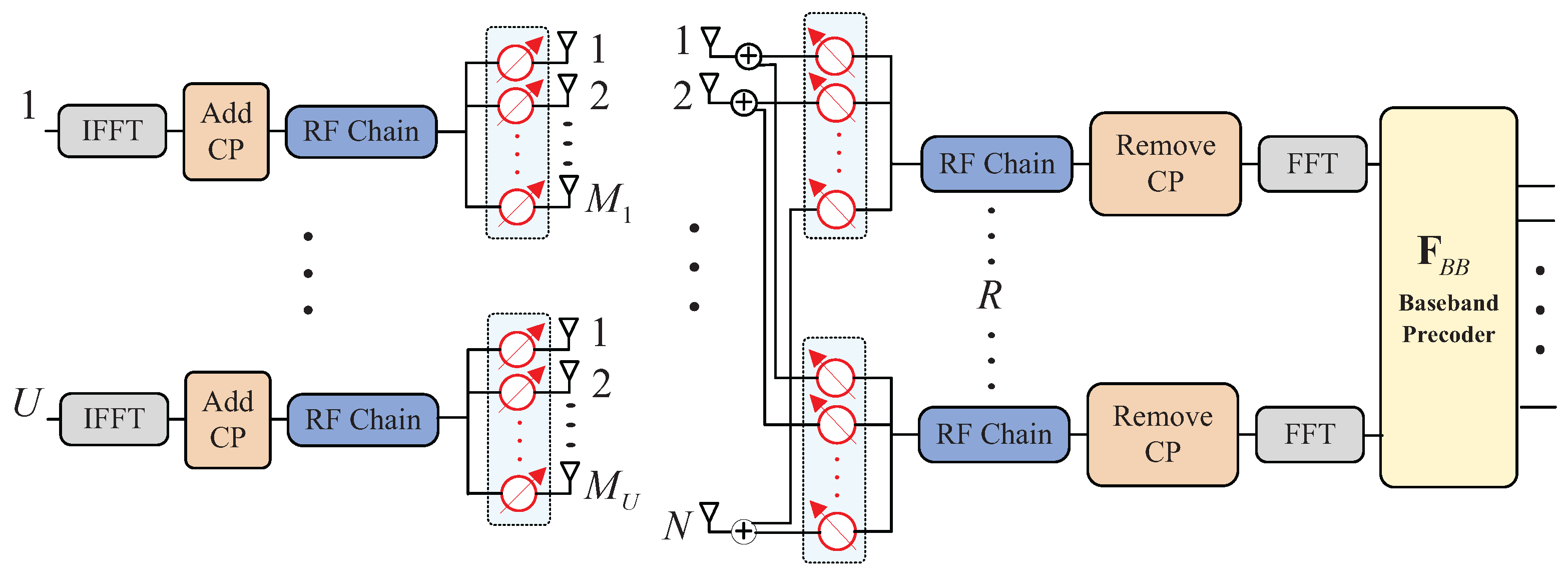
2. System Model
2.1. PARAFAC Model
2.2. Constructed PARAFAC Model
2.3. Uniqueness Issue
3. Proposed PARAFAC Decomposition-Based Channel Estimation Scheme
3.1. The ATALS Algorithm
3.2. Channel Parameter Extraction
| Algorithm 1 PARAFAC decomposition-based channel estimation algorithm |
| Input: Received tensor , precoding matrix , combining matrix , one-dimensional search number J, the number of paths of U MSs and error threshold . |
| Output: Estimates , , and . |
| First stage (the ATALS algorithm): |
| Initialization: Randomly initialize , , , , , . Set , and . |
| Step 1.1. Compute from (25) with , and compare it with from (20). |
| If , construct , , with ; else, construct , , with . |
| Step 1.2. Update using , , by . |
| Step 1.3. Update using , , by . |
| Step 1.4. Update using , , by . |
| Step 1.5. Compute the new error . If , then end. |
| Otherwise, set and go to Step 1.1.. |
| Second stage (Channel parameter extraction via one-dimension search): |
| for, and for |
| Step 2.1. Estimate the AoA by (27) with , . |
| Step 2.2. Estimate the AoD by (28) with , . |
| Step 2.3. Estimate the delay by (29) with , . |
| Step 2.4. Compute the diagonal matrices , and . |
| Step 2.5. Estimate the path gain according to . |
4. Cramér–Rao Bound Deriavtion
5. System Performance Analysis
5.1. Analysis of Computational Complexity
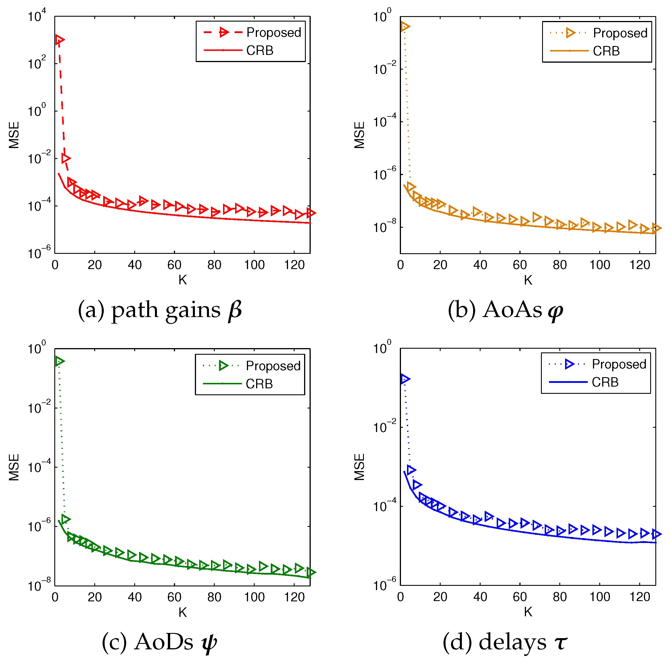
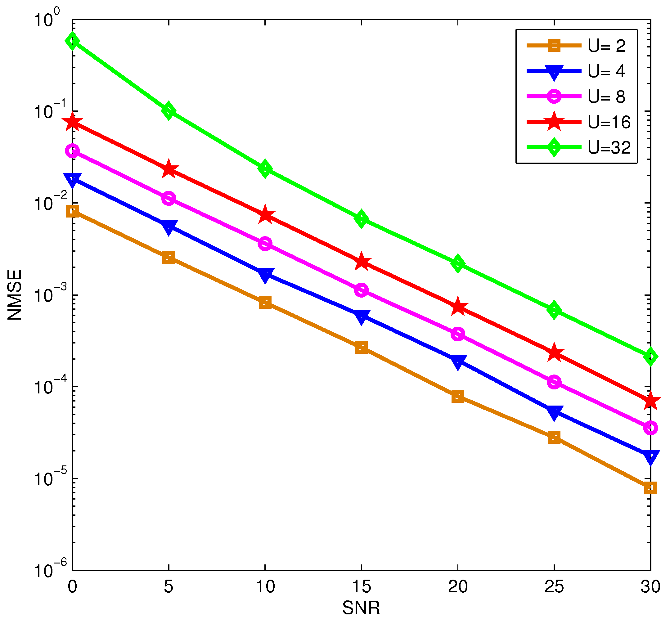
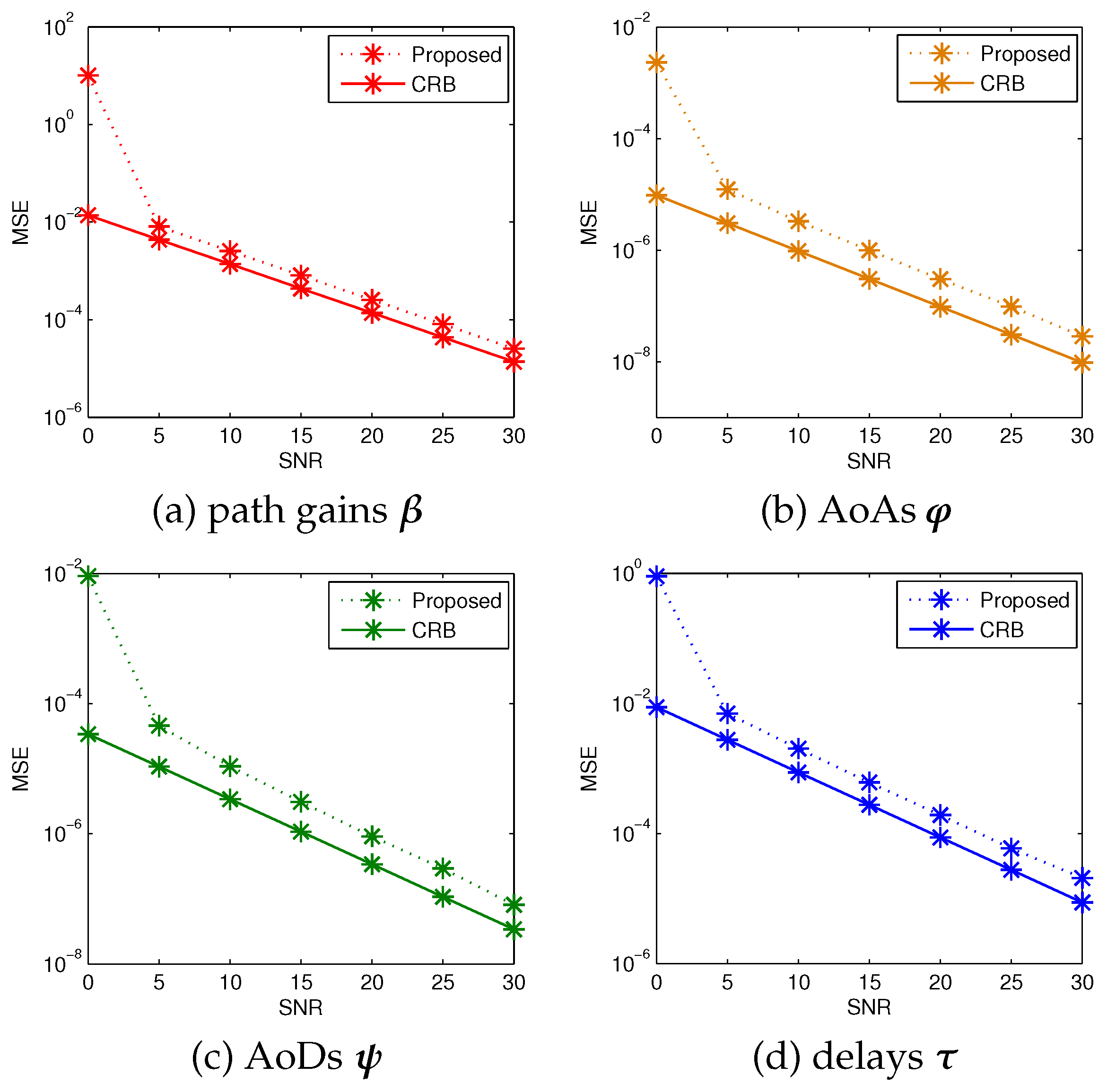
5.2. Simulation Results
6. Conclusions
Author Contributions
Funding
Acknowledgments
Conflicts of Interest
Abbreviations
| ALS | alternating least squares |
| AoAs | angles of arrival |
| AoDs | angles of departure |
| ATALS | accelerated trilinear alternating least squares |
| BS | base station |
| CP | CANDECOMP/PARAFAC |
| CRB | Cramér–Rao Bound |
| CS | compressing sensing |
| eMBB | extended mobile broadband |
| FSF | frequency-selective fading |
| IoT | internet of things |
| MIMO | multiple-input multiple-output |
| mMTC | massive machine-type communication |
| MMV | multiple measurement vector |
| mmWave | millimeter wave |
| MS | mobile station |
| MSEs | mean square errors |
| OFDM | orthogonal frequency divisional multiplexing |
| OMP | orthogonal matching pursuit |
| PARAFAC | parallel factor |
| RF | radio frequency |
| SOMP | simultaneous orthogonal matching pursuit |
| ULA | uniform linear array |
| UPA | uniform planar array |
| URLLC | ultra-reliable low-latency communication |
Appendix A. Derivation of Cramér–Rao Bound
References
- Rappaport, T.S.; Sun, S.; Mayzus, R.; Zhao, H.; Azar, Y.; Wang, K.; Wong, G.N.; Schulz, J.K.; Samimi, M.; Gutierrez, F. Millimeter Wave Mobile Communications for 5G Cellular: It Will Work! IEEE Access 2013, 1, 335–349. [Google Scholar] [CrossRef]
- Swindlehurst, A.L.; Ayanoglu, E.; Heydari, P.; Capolino, F. Millimeter-wave massive MIMO: The next wireless revolution? IEEE Commun. Mag. 2014, 52, 56–62. [Google Scholar] [CrossRef]
- Pi, Z.; Choi, J.; Heath, R. Millimeter-wave gigabit broadband evolution toward 5G: Fixed access and backhaul. IEEE Commun. Mag. 2016, 54, 138–144. [Google Scholar] [CrossRef]
- Ciuonzo, D.; Rossi, P.S.; Dey, S. Massive MIMO Channel-Aware Decision Fusion. IEEE Trans. Signal Process. 2015, 63, 604–619. [Google Scholar] [CrossRef]
- Bana, A.S.; Carvalho, E.D.; Soret, B.; Abrão, T.; Marinello, J.C.; Larsson, E.G.; Popovski, P. Massive MIMO for Internet of Things (IoT) connectivity. Phys. Commun. 2019, 37, 100859–100875. [Google Scholar] [CrossRef] [Green Version]
- Dey, I.; Ciuonzo, D.; Rossi, P.S. Wideband Collaborative Spectrum Sensing Using Massive MIMO Decision Fusion. IEEE Trans. Wirel. Commun. 2020, 19, 5246–5260. [Google Scholar] [CrossRef]
- Tsang, Y.M.; Poon, A.S.Y.; Addepalli, S. Coding the Beams: Improving Beamforming Training in mmWave Communication System. In Proceedings of the 2011 IEEE Global Telecommunications Conference—GLOBECOM 2011, Houston, TX, USA, 5–9 December 2011; pp. 1–6. [Google Scholar]
- Kutty, S.; Sen, D. Beamforming for Millimeter Wave Communications: An Inclusive Survey. IEEE Commun. Surv. Tutor. 2016, 18, 949–973. [Google Scholar] [CrossRef]
- Han, S.; Chih-Lin, I.; Xu, Z.; Rowell, C. Large-scale antenna systems with hybrid analog and digital beamforming for millimeter wave 5G. IEEE Commun. Mag. 2015, 53, 186–194. [Google Scholar] [CrossRef]
- Alkhateeb, A.; El Ayach, O.; Leus, G.; Heath, R.W. Channel Estimation and Hybrid Precoding for Millimeter Wave Cellular Systems. IEEE J. Sel. Top. Signal Process. 2014, 8, 831–846. [Google Scholar] [CrossRef] [Green Version]
- Gao, Z.; Dai, L.; Mi, D.; Wang, Z.; Imran, M.A.; Shakir, M.Z. MmWave massive-MIMO-based wireless backhaul for the 5G ultra-dense network. IEEE Wirel. Commun. 2015, 22, 13–21. [Google Scholar] [CrossRef] [Green Version]
- Gao, X.; Dai, L.; Han, S.; Chih-Lin, I.; Heath, R.W. Energy-Efficient Hybrid Analog and Digital Precoding for MmWave MIMO Systems with Large Antenna Arrays. IEEE J. Sel. Areas Commun. 2016, 34, 998–1009. [Google Scholar] [CrossRef] [Green Version]
- Kassam, J.; Miri, M.; Magueta, R.; Castanheira, D.; Gameiro, A. Two-Step Multiuser Equalization for Hybrid mmWave Massive MIMO GFDM Systems. Electronics 2020, 9, 1220. [Google Scholar] [CrossRef]
- Magueta, R.; Castanheira, D.; Pedrosa, P.; Silva, A.; Dinis, R.; Gameiro, A. Iterative Analog–Digital Multi-User Equalizer for Wideband Millimeter Wave Massive MIMO Systems. Sensors 2020, 20, 575. [Google Scholar] [CrossRef] [Green Version]
- Alkhateeb, A.; Heath, R.W. Frequency Selective Hybrid Precoding for Limited Feedback Millimeter Wave Systems. IEEE Trans. Commun. 2016, 64, 1801–1818. [Google Scholar] [CrossRef] [Green Version]
- Ngo, H.Q.; Larsson, E.G.; Marzetta, T.L. Energy and Spectral Efficiency of Very Large Multiuser MIMO Systems. IEEE Trans. Commun. 2013, 61, 1436–1449. [Google Scholar]
- Zhang, J.; Dai, L.; Sun, S.; Wang, Z. On the Spectral Efficiency of Massive MIMO Systems with Low-Resolution ADCs. IEEE Commun. Lett. 2016, 20, 842–845. [Google Scholar] [CrossRef] [Green Version]
- Jin, S.; Liang, X.; Wong, K.K.; Gao, X.; Zhu, Q. Ergodic Rate Analysis for Multipair Massive MIMO Two-Way Relay Networks. IEEE Trans. Wirel. Commun. 2015, 14, 1480–1491. [Google Scholar] [CrossRef]
- Hur, S.; Kim, T.; Love, D.J.; Krogmeier, J.V.; Thomas, T.A.; Ghosh, A. Millimeter Wave Beamforming for Wireless Backhaul and Access in Small Cell Networks. IEEE Trans. Commun. 2013, 61, 4391–4403. [Google Scholar] [CrossRef] [Green Version]
- Kim, T.; Love, D.J. Virtual AoA and AoD estimation for sparse millimeter wave MIMO channels. In Proceedings of the 2015 IEEE 16th International Workshop on Signal Processing Advances in Wireless Communications (SPAWC), Stockholm, Sweden, 27 June–1 July 2015; pp. 146–150. [Google Scholar]
- Heath, R.W.; González-Prelcic, N.; Rangan, S.; Roh, W.; Sayeed, A.M. An Overview of Signal Processing Techniques for Millimeter Wave MIMO Systems. IEEE J. Sel. Top. Signal Process. 2016, 10, 436–453. [Google Scholar] [CrossRef]
- Schniter, P.; Sayeed, A. Channel estimation and precoder design for millimeter-wave communications: The sparse way. In Proceedings of the 2014 48th Asilomar Conference on Signals, Systems and Computers, Pacific Grove, CA, USA, 2–5 November 2014; pp. 273–277. [Google Scholar]
- Gao, X.; Dai, L.; Zhou, S.; Sayeed, A.M.; Hanzo, L. Beamspace Channel Estimation for Wideband Millimeter-Wave MIMO with Lens Antenna Array. In Proceedings of the 2018 IEEE International Conference on Communications (ICC), Kansas City, MO, USA, 20–24 May 2018; pp. 1–6. [Google Scholar]
- Cheng, L.; Yue, G.; Yu, D.; Liang, Y.; Li, S. Millimeter Wave Time-Varying Channel Estimation via Exploiting Block-Sparse and Low-Rank Structures. IEEE Access 2019, 7, 123355–123366. [Google Scholar] [CrossRef]
- Fazal-E-Asim; Antreich, F.; Cavalcante, C.C.; de Almeida, A.L.F.; Nossek, J.A. Two-Dimensional Channel Parameter Estimation for Millimeter-Wave Systems Using Butler Matrices. IEEE Trans. Wirel. Commun. 2021, 20, 2670–2684. [Google Scholar] [CrossRef]
- Bajwa, W.U.; Haupt, J.; Sayeed, A.M.; Nowak, R. Compressed Channel Sensing: A New Approach to Estimating Sparse Multipath Channels. Proc. IEEE 2010, 98, 1058–1076. [Google Scholar] [CrossRef]
- Nguyen, S.L.H.; Ghrayeb, A. Compressive sensing-based channel estimation for massive multiuser MIMO systems. In Proceedings of the 2013 IEEE Wireless Communications and Networking Conference (WCNC), Shanghai, China, 7–10 April 2013; pp. 2890–2895. [Google Scholar]
- Alkhateeb, A.; Leus, G.; Heath, R.W. Compressed sensing based multi-user millimeter wave systems: How many measurements are needed? In Proceedings of the 2015 IEEE International Conference on Acoustics, Speech and Signal Processing (ICASSP), Brisbane, Australia, 19–24 April 2015; pp. 2909–2913. [Google Scholar]
- Xie, H.; Gao, F.; Zhang, S.; Jin, S. A Unified Transmission Strategy for TDD/FDD Massive MIMO Systems with Spatial Basis Expansion Model. IEEE Trans. Veh. Technol. 2017, 66, 3170–3184. [Google Scholar] [CrossRef]
- Wang, S.; Li, Y.; Wang, J. Multiuser Detection in Massive Spatial Modulation MIMO with Low-Resolution ADCs. IEEE Trans. Wirel. Commun. 2015, 14, 2156–2168. [Google Scholar] [CrossRef]
- Zhang, J.; Podkurkov, I.; Haardt, M.; Nadeev, A. Channel Estimation and Training Design for Hybrid Analog-Digital Multi-Carrier Single-User Massive MIMO Systems. In Proceedings of the WSA 2016; 20th International ITG Workshop on Smart Antennas, Munich, Germany, 9–11 March 2016; pp. 1–8. [Google Scholar]
- You, L.; Gao, X.; Swindlehurst, A.L.; Zhong, W. Channel Acquisition for Massive MIMO-OFDM with Adjustable Phase Shift Pilots. IEEE Trans. Signal Process. 2016, 64, 1461–1476. [Google Scholar] [CrossRef]
- Wei, X.; Peng, W.; Ng, D.; Robert, S.; Jiang, T. Joint Estimation of Channel Parameters in Massive MIMO Systems via PARAFAC Analysis. In Proceedings of the 2018 International Conference on Computing, Networking and Communications (ICNC), Maui, HI, USA, 5–8 March 2018; pp. 496–502. [Google Scholar]
- Wei, X.; Peng, W.; Chen, D.; Ng, D.; Jiang, T. Joint Channel Parameter Estimation in Multi-Cell Massive MIMO System. IEEE Trans. Commun. 2019, 67, 3251–3264. [Google Scholar] [CrossRef]
- Zhou, Z.; Fang, J.; Yang, L.; Li, H.; Chen, Z.; Li, S. Channel Estimation for Millimeter-Wave Multiuser MIMO Systems via PARAFAC Decomposition. IEEE Trans. Wirel. Commun. 2016, 15, 7501–7516. [Google Scholar] [CrossRef]
- Gao, Z.; Hu, C.; Dai, L.; Wang, Z. Channel Estimation for Millimeter-Wave Massive MIMO with Hybrid Precoding Over Frequency-Selective Fading Channels. IEEE Commun. Lett. 2016, 20, 1259–1262. [Google Scholar] [CrossRef] [Green Version]
- Venugopal, K.; Alkhateeb, A.; González Prelcic, N.; Heath, R.W. Channel Estimation for Hybrid Architecture-Based Wideband Millimeter Wave Systems. IEEE J. Sel. Areas Commun. 2017, 35, 1996–2009. [Google Scholar] [CrossRef]
- Zhou, Z.; Fang, J.; Yang, L.; Li, H.; Chen, Z.; Blum, R.S. Low-Rank Tensor Decomposition-Aided Channel Estimation for Millimeter Wave MIMO-OFDM Systems. IEEE J. Sel. Areas Commun. 2017, 35, 1524–1538. [Google Scholar] [CrossRef]
- Akdeniz, M.R.; Liu, Y.; Samimi, M.K.; Sun, S.; Rangan, S.; Rappaport, T.S.; Erkip, E. Millimeter Wave Channel Modeling and Cellular Capacity Evaluation. IEEE J. Sel. Areas Commun. 2014, 32, 1164–1179. [Google Scholar] [CrossRef]
- Rajih, M.; Comon, P. Enhanced Line Search: A novel method to accelerate Parafac. In Proceedings of the 2005 13th European Signal Processing Conference, Antalya, Turkey, 4–8 September 2005; pp. 1–4. [Google Scholar]
- Liu, X.; Sidiropoulos, N. Cramer–Rao lower bounds for low-rank decomposition of multidimensional arrays. IEEE Trans. Signal Process. 2001, 49, 2074–2086. [Google Scholar]
- Zhou, Y.; Cheung, Y.M. Bayesian Low-Tubal-Rank Robust Tensor Factorization with Multi-Rank Determination. IEEE Trans. Pattern Anal. Mach. Intell. 2021, 43, 62–76. [Google Scholar] [CrossRef]


| Works | System Scenario | Algorithm |
|---|---|---|
| [36] | multiuser mmWave massive MIMO-OFDM system | SOMP |
| [37] | mmWave massive MIMO-OFDM system | OMP |
| [38] | mmWave massive MIMO-OFDM system | adaptive CS |
| [10] | mmWave massive MIMO system | CP decomposition-based method |
| our work | multiuser mmWave massive MIMO-OFDM system | PARAFAC-based channel parameter estimation |
| Algorithm | Complexity | |
|---|---|---|
| SOMP | ||
| OMP | ||
| Adaptive CS | ||
| Proposed | First stage | |
| Second stage | ||
| Total | ||
| System Parameter | Configuration |
|---|---|
| BS antennas N/RF chains R | 64/10 |
| MS antennas M/RF chains | 32/1 |
| Transmission subcarriers K | 128 |
| Total number of MSs U/paths | 6/8 |
| Carrier frequency | 28 GHz |
| Sampling rate | 0.25 GHz |
| AoA/AoD / | |
| Path gain | |
| Delay |
| SNR(dB) | 0 | 5 | 10 | 15 | 20 | 25 | 30 |
|---|---|---|---|---|---|---|---|
| SOMP (R = 8) | 1.1239 s | 1.1892 s | 1.1923 s | 1.2035 s | 1.2315 s | 1.2174 s | 1.2248 s |
| OMP (R = 8) | 2.2667 s | 2.2075 s | 2.2738 s | 2.2493 s | 2.2512 s | 2.2555 s | 2.2542 s |
| Adaptive CS (R = 8) | 1.0299 s | 0.9888 s | 1.1948 s | 1.1877 s | 1.2464 s | 1.2162 s | 1.1911 s |
| Proposed (R = 8) | 0.7117 s | 0.6612 s | 0.595 s | 0.7766 s | 0.7377 s | 0.6304 s | 0.6987 s |
| SOMP (R = 16) | 1.635 s | 1.5626 s | 1.6055 s | 1.6113 s | 1.5785 s | 1.6153 s | 1.6129 s |
| OMP (R = 16) | 5.3028 s | 5.3577 s | 5.2848 s | 5.2799 s | 5.328 s | 5.4576 s | 5.3256 s |
| Adaptive CS (R = 16) | 1.4869 s | 1.679 s | 1.6707 s | 1.678 s | 1.6739 s | 1.7011 s | 1.6774 s |
| Proposed (R = 16) | 0.7749 s | 0.8524 s | 0.8869 s | 0.8478 s | 0.8686 s | 0.8329 s | 0.8868 s |
Publisher’s Note: MDPI stays neutral with regard to jurisdictional claims in published maps and institutional affiliations. |
© 2021 by the authors. Licensee MDPI, Basel, Switzerland. This article is an open access article distributed under the terms and conditions of the Creative Commons Attribution (CC BY) license (https://creativecommons.org/licenses/by/4.0/).
Share and Cite
Chang, R.; Yuan, C.; Du, J. PARAFAC-Based Multiuser Channel Parameter Estimation for MmWave Massive MIMO Systems over Frequency Selective Fading Channels. Electronics 2021, 10, 2983. https://doi.org/10.3390/electronics10232983
Chang R, Yuan C, Du J. PARAFAC-Based Multiuser Channel Parameter Estimation for MmWave Massive MIMO Systems over Frequency Selective Fading Channels. Electronics. 2021; 10(23):2983. https://doi.org/10.3390/electronics10232983
Chicago/Turabian StyleChang, Rui, Chaowei Yuan, and Jianhe Du. 2021. "PARAFAC-Based Multiuser Channel Parameter Estimation for MmWave Massive MIMO Systems over Frequency Selective Fading Channels" Electronics 10, no. 23: 2983. https://doi.org/10.3390/electronics10232983
APA StyleChang, R., Yuan, C., & Du, J. (2021). PARAFAC-Based Multiuser Channel Parameter Estimation for MmWave Massive MIMO Systems over Frequency Selective Fading Channels. Electronics, 10(23), 2983. https://doi.org/10.3390/electronics10232983