Article

Design Space Exploration of Hybrid Quantum–Classical Neural Networks

Division of Information and Computing Technology, College of Science and Engineering, Hamad Bin Khalifa University, Qatar Foundation, Doha P.O. Box 34110, Qatar
*
Author to whom correspondence should be addressed.
Electronics 2021, 10(23), 2980; https://doi.org/10.3390/electronics10232980
Submission received: 23 October 2021 / Revised: 17 November 2021 / Accepted: 22 November 2021 / Published: 30 November 2021
(This article belongs to the Special Issue Quantum Machine Learning: Theory, Methods and Applications)

Abstract

:
The unprecedented success of classical neural networks and the recent advances in quantum computing have motivated the research community to explore the interplay between these two technologies, leading to the so-called quantum neural networks. In fact, universal quantum computers are anticipated to both speed up and improve the accuracy of neural networks. However, whether such quantum neural networks will result in a clear advantage on noisy intermediate-scale quantum (NISQ) devices is still not clear. In this paper, we propose a systematic methodology for designing quantum layer(s) in hybrid quantum–classical neural network (HQCNN) architectures. Following our proposed methodology, we develop different variants of hybrid neural networks and compare them with pure classical architectures of equivalent size. Finally, we empirically evaluate our proposed hybrid variants and show that the addition of quantum layers does provide a noticeable computational advantage.

1. Introduction

Machine learning (ML) is the subfield of artificial intelligence (AI) that entails programming computers to learn from data [1]. Among others, neural networks are one of the most widely used ML models, providing clear advantages including adaptive learning, self-organization, real-time operation, parallelism and fault tolerance [2]. Deep learning is an extension of neural networks with a greater number of hidden neuron layers, and this technique is well suited for learning from large amounts of data, often referred to as big data [3]. Over the years, many powerful deep neural networks (DNNs) models have been proposed and have been shown to exhibit exceptional performance in a variety of scenarios. Examples of applications where deep learning outperforms other state-of-the-art ML algorithms include speech recognition [4,5], computer vision [6,7], natural language processing [8], cybersecurity [9] and healthcare [10,11], to name a few.
The primary objective when designing DNN architectures is the efficient optimization of the network in such a way that it leads to better training accuracy (how well the model learns from the data) and validation accuracy (the model’s performance on unseen data) [12,13,14]. Another important performance metric in DNNs is the model generalization (how efficiently the model adapts to new unseen data) [15], which is the difference between the training and validation accuracy given that we have a large enough dataset for training the model and vice versa to avoid the issues of underfitting (low training accuracy and low validation accuracy) and overfitting (high training accuracy and low validation accuracy). Ignoring underfitting and overfitting, the generalization error can be defined as in Equation (1).
G e n e r a l i z a t i o n E r r o r ( % ) = T r a i n A c c u r a c y V a l i d a t i o n A c c u r a c y T r a i n A c c u r a c y × 100
The smaller the difference between the train and validation accuracy, the better the generalization. If the generalization error of a model is high, it means that the model is not actually learning, rather just memorizing the data. Consequently, the model will fail to efficiently predict using data it has not seen before. The convergence time (the time the model takes to reach an optimal performance) of neural networks is another important performance metric when dealing with real-world datasets, which should be reasonably practical.
In recent years, research in quantum computing has advanced considerably, mainly motivated by its potential to outperform classical computation for certain tasks. In fact, regarding quantum supremacy, refs. [16,17,18] recently provided practical evidence of the computational advantage of quantum over classical computers. These successful experimental illustrations of quantum supremacy motivated the research community to explore the extent to which quantum computing can improve ML, which is today termed as quantum machine learning (QML). QML has become an interesting research topic, and various ML algorithms are being developed in the quantum realm. The primary purpose of QML is to explore and analyze the possible advantages quantum computation might offer to ML compared to classical ML algorithms.
Universal fault-tolerant quantum computers are anticipated to significantly enhance the performance of machine learning algorithms. Although the quest for building a universal fault tolerant quantum computer has had a great deal of effort devoted to it over the last decade and various important advances and milestones have been achieved, a universal fault-tolerant quantum computer is still not expected in the near future. However, small-scale quantum computers with limited numbers of qubits and with small resilience to noise have already been developed [19,20]. These small-scale quantum computers fall into the noisy intermediate scale quantum computation (NISQ) regime, and such quantum devices are not yet proven to enhance the performance of machine learning algorithms. However, significant progress has been made in QML [21,22,23,24], particularly quantum neural networks (QNNs) [25,26,27,28,29,30,31,32] for various applications including image generation [33,34,35] and data classification [23]. QNNs are also being explored in terms of their trainability and generalization [36,37,38,39,40,41,42]. For example, a recent work [39] investigated QNNs for NISQ devices and analyzed how a well-designed QNN can outperform classical neural networks in terms of data expressibility (the types of functions a neural network architecture can fit). Similarly, in [43], QNNs have also been designed and analyzed on real-world datasets including MNIST [44]. However, some claims have been made in the literature proposing the advantage of QNN over classical NNs [43].
The main objective of quantum machine learning algorithms is to achieve better trainability and generalization with a reasonable model convergence time (at least compared with the classical machine learning algorithms). However, in the NISQ era, building better quantum machine learning models than their classical counterparts might be a challenge because of two fundamental problems: (1) the unavailability of native quantum datasets and (2) the unavailability of quantum memory (QRAM) and sufficiently strong quantum processors for storing and handling big data. While this limits the progress of developing standalone and sufficiently strong QNNs, it has motivated a hybrid quantum–classical approach [
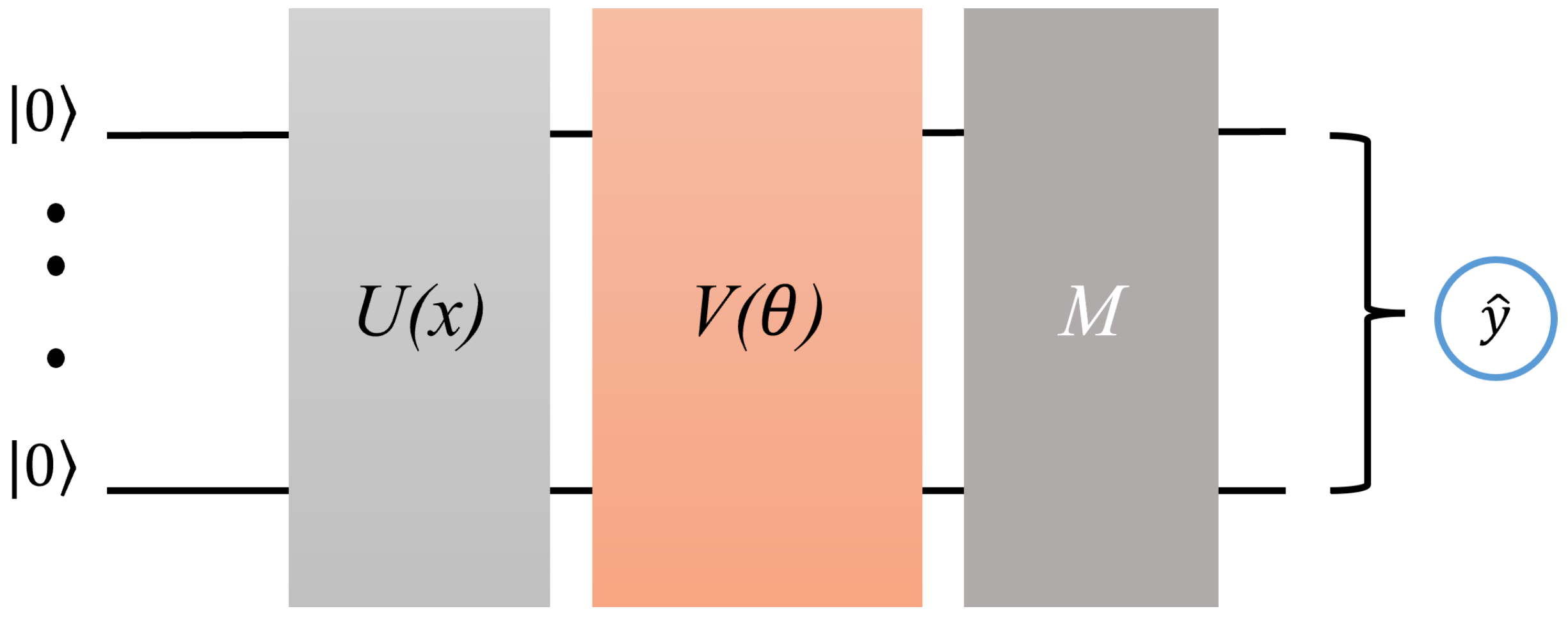
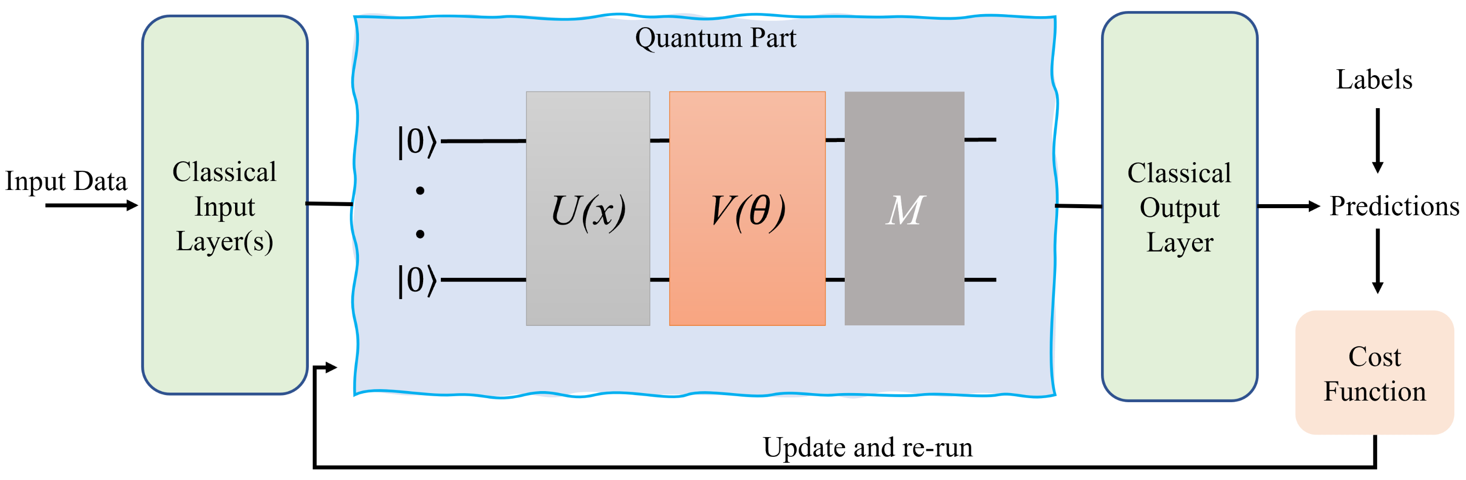
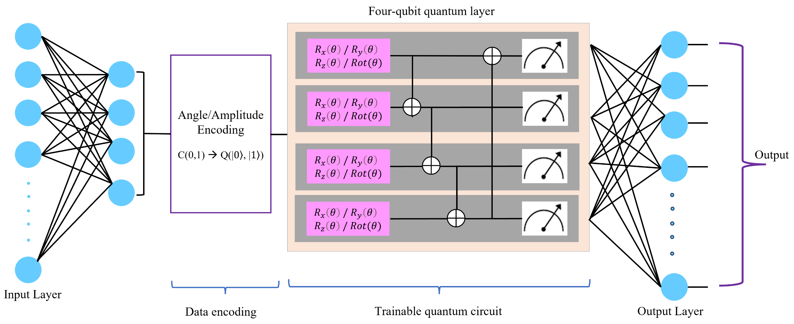
26], which is now widely used to achieve a reasonable quantum advantage in neural networks. The hybrid quantum–classical neural networks (HQCNNs) follow the same architecture as QNNs, as shown in Figure 1, while including classical input and output layers. The input layers reduce the input data dimension before being encoded into the quantum circuit, while the output layer is used to classically post-process the measurement results of the quantum circuit. Furthermore, HQCNNs are also possible to simulate on NISQ platforms and use variational quantum circuits due to their robustness against noise on NISQ devices [45,46,47,48]. We discuss HQCNNs and variational quantum circuits further in Section 2.1 and Section 2.4.
Some studies have claimed that QNNs can surpass classical DNNs for particular learning tasks, such as the discrete logarithm problem [38], and quantum synthetic data classification [23]. However, a relatively recent work [49] criticized these claims and discussed the barren plateau problem (the problem of vanishing gradients) in QNNs, which poses a limitation on the applicability of QNNs for large-scale real-world problems. This limitation of QNNs makes it unclear whether or not the QNNs can provide any advantage over their classical counterparts. However, recently there have been some efforts to understand and overcome the issue of barren plateaus in QNNs [50,51], opening the doors for real world applications of QNNs.
There is still no standard methodology to design quantum circuits for QNNs, which we speculate is one reason behind the mixed opinions of the quantum advantage in QNNs. Therefore, it is crucial to develop a systematic approach to design quantum circuits for QNNs rather than relying on heuristics.

1.1. Contribution

Realizing the fact that the quantum part of HQCNNs is largely unexplored, in this paper, we perform a comprehensive Design Space Exploration (DSE) of quantum circuit construction in HQCNNs. To illustrate this process, we use image classification problems. We also demonstrate the practical quantum advantage of HQCNNs over pure classical networks in terms of computational efficiency and comparable accuracy. We use various commonly used parameterized quantum gates, particularly in the context of QNNs, with different data encoding techniques (specifically, amplitude and angle encoding), which gives us the best set of quantum gates with corresponding encoding techniques. We also develop different variants of HQCNNs with a maximum of four qubits (for a fair comparison with classical counterpart), progressing from simpler to more sophisticated quantum circuits. The primary objective of this exercise is to reduce the trial efforts required for designing quantum circuits for HQCNNs.

1.2. Organization

The rest of the paper is organized as follows: Section 2 contains the necessary background and terminologies used in this paper. Our proposed hybrid HQCNN variants are introduced in Section 3. The evaluation results and brief comparisons of all the hybrid and classical counterparts are presented in Section 4 and Section 5, respectively. Finally, Section 7 concludes the paper.

2. Preliminaries

2.1. Hybrid Quantum–Classical Neural Networks (HQCNN)

In HQCNNs, part of the neural network is made quantum. A typical structure of a hybrid QNN consists of a trainable variational quantum circuit sandwiched between input and output classical neural layers. In this architecture, the quantum circuit serves as the hidden layers of the HQCNN. The quantum part in HQCNNs is similar to the original QNN architecture and consists of two parts: (1) data encoding, which encodes the classical data, and (2) a trainable variational quantum circuit. An abstract illustration of an HQCNN is shown in Figure 2.
The classical input layers in the HQCNN architecture are usually used to downsize the input feature space to make it compatible for NISQ devices. The quantum part is similar to QNN (Figure 1). The classical output layer is typically used to classically post-process the measurement results of the quantum part. Moreover, in HQCNNs, the parameters can also be updated classically since the measurements returned from the quantum part are classical values.

2.2. Dataset Preparation

In this paper, we use MNIST handwritten digits dataset for training the HQCNNs. The standard MNIST dataset has 60,000 training images and 10,000 testing images. This dataset is quite large for HQCNNs on NISQ devices. Therefore, we create two subsets from the original dataset: a small dataset (D103) containing 10,000 training and 3000 test images, and a large dataset (D204) containing 20,000 training and 4000 test images. The pure classical neural network and all the variants of HQCNNs are trained for both D103 and D204.

2.3. Data Encoding

Machine learning depends heavily on big data. In the current NISQ era, we have a very limited number of qubits available and almost no diverse quantum datasets. Hence, we rely on classical datasets, which are required to be encoded. Encoding can be considered as data point ( x χ ) loading from memory into a quantum state so that a QML algorithm (e.g., quantum neural network) can process it.
From a practical viewpoint, data encoding is performed via a unitary [52] state preparation circuit S x , which is realized in terms of single and double qubit gates acting on an initial state | ϕ , which is usually the all zero state | ϕ = | 0 n . The encoding can then be represented by Equation (2).
x E ( x ) = S x | ϕ ϕ | S x = | x x | = : ρ x
For S x to be suitable for the data encoding, it is required that the gates count is polynomial (or sub-polynomial) compared to the number of qubits. Moreover, the state preparation circuit needs to be hardware efficient; that is, the single and double quantum gates can be realized efficiently without increasing the overhead cost.
Different techniques are used to encode the data into an n-qubit quantum device, namely amplitude, angle, basis, qsample and dynamic encoding. Below, we briefly introduce amplitude and angle encoding strategies, as these are the most popular and the strategies we adopt in this work. The details on other encoding techniques can be found in [53].

2.3.1. Amplitude Encoding

Amplitude encoding associates classical information, such as a real vector, with quantum amplitudes. This can be achieved in various ways. For instance, a classical normalized vector x C 2 n , k | x | 2 = 1 can be encoded in the amplitudes of quantum state as shown in Equation (3).
x 1 x 2 n | ψ x = j = 1 2 n x j | j
Similarly, a classical matrix A C 2 n × C 2 n with entries a i j that fulfill i j | a i j | 2 = 1 can be represented by accordingly enlarging the Hilbert space, as shown in Equation (4).
| ψ A = i = 1 2 m j = 1 2 n a i j | i | j
One of the limitations of amplitude encoding is that it can process only normalized classical vectors, which eventually leads to data representation in one fewer dimension (e.g., a classical 2-dimensional vector ( x 1 , x 2 ) T can only be associated with an amplitude vector ( α 1 , α 2 ) T of a qubit, which fulfills | α 1 | 2 + | α 2 | 2 = 1 ). This means that it lies on a unit circle—a one-dimensional shape in two-dimensional space.

2.3.2. Angle Encoding

Another popular data encoding technique for classical–quantum hybrid algorithms is angle encoding [53]. Angle encoding [53], sometimes also called “qubit encoding”, has been used widely in a number of recent QML experiments [54,55,56]. In angle encoding, the features are encoded into the rotation angle of qubits and can be represented by the following equation [52]:
| x = i = 1 N c o s ( x i ) | 0 + s i n ( x i ) | 1
This encoding technique makes use of N qubits with a quantum circuit of constant depth, which makes it more suitable for NISQ devices. The state preparation unitary in the case of angle encoding encodes a single feature per qubit, as shown in Equation (6) :
S x j = i = 1 N U i w h e r e U i : = cos ( x j ( i ) ) sin ( x j ( i ) ) sin ( x j ( i ) ) cos ( x j ( i ) )

2.4. Variational Quantum Circuits for HQCNNs

The variational circuit V ( θ ) is an ansatz (a subroutine consisting of a sequence of gates applied to specific wires) which defines a set of all possible states | ψ ( θ ) it is able to prepare. In the QML context, the idea of hybrid training is to use a quantum device with some classical processing to compute the objective function c ( θ ) for a given set of parameters θ . Afterwards, a classical algorithm optimizes the parameters by making queries to the quantum device [57]. The parameterized circuit V ( θ ) is implemented by a quantum device which then prepares a state V ( θ ) | 0 = | ψ ( θ ) according to the circuit parameters θ . The final state measurements V ( θ ) give the state or expectation value estimates of a particular qubit, which depends on the circuit parameters θ . These expectation values are then used by the cost function C ( θ ) , which determines how good θ is in the context of the problem under consideration. The main objective of the algorithm is to find the optimal circuit parameters θ of the variational circuit, which would tend to minimize C ( θ ) . Analogous to the objective of selecting a suitable model in conventional machine learning, choosing an efficient ansatz that allows the parameterized state to approximate possible solutions to the problem by using fewer parameters is a challenging task in QML.
Variational quantum circuits have recently become a very popular approach for QML applications on NISQ devices because of a number of advantages [53]:
  • Only a small portion of the overall algorithm is required to run coherently (as a quantum circuit), leading to smaller circuit;
  • Since there are many possible ansatzes, it is possible to design the circuit based on the underlying device capabilities;
  • Since the circuit is learnable, it can add robustness against device errors. For instance, if a certain state is over-rotated, it can be automatically corrected by parameter self-adjustment.

3. Methodology

The methodology to design efficient quantum circuits in hybrid quantum–classical neural networks (HQCNNs) is not very well-defined in the literature, and that might be one of the important reasons behind the mixed opinions regarding the potential advantage of quantum computation in HQCNNs. In this paper, we develop different variants of HQCNNs and perform a comprehensive analysis of how various encoding techniques and quantum gates/circuits potentially affect the performance of these hybrid networks. This exercise will reduce the trial efforts required to select quantum gates (for quantum circuit design) and encoding techniques (encoding the data into quantum system) in HQCNNs for a specific application. Furthermore, we also compare the hybrid networks with their classical counterparts to determine whether the quantum layers introduce any advantage. In particular, we train the same model on both D103 and D204 to observe and compare the convergence rate and whether there is any computational advantage in the hybrid case. We also compare the models in terms of the overall accuracy and generalization error improvement rate.
For all the models (hybrid and classical), we use the Adam optimizer with an initial learning rate of 0.01. Moreover, the learning is scheduled for better training, and we use the early stopping method in keras to avoid overfitting. The maximum number of training epochs is set to 100; however, if there is no improvement in validation loss for three consecutive epochs, the learning rate scheduler reduces the learning rate by a factor of 0.1, and the new learning is calculated as shown in Equation (7). If there is no improvement in validation loss for four consecutive epochs, the training is stopped to avoid overfitting.
n e w l e a r n i n g r a t e = p r e v i o u s l e a r n i n g r a t e × 0.1
The hybrid architectures we use in our experiments consist of two input layers. The first layer completely encodes the input features, and the following classical layer consists of four neurons, downsizing the feature size being encoded into the quantum circuit. The last classical layer of all the hybrid model consists of 10 neurons because the dataset we are using (MNIST) consists of 10 output classes. The qubit measurements are performed in the eigen-basis of σ z for all the variants of implemented HQCNNs. In addition, for the angle encoding, the rotation gate used to encode features in qubit rotations is R x ( θ ) for all hybrid networks. In the following sections, we discuss in detail all our HQCNN variants and two classical counterparts. It is important to note here that we keep the number of qubits the same in all the variants of the HQCCNs to allow a fair comparison between them.

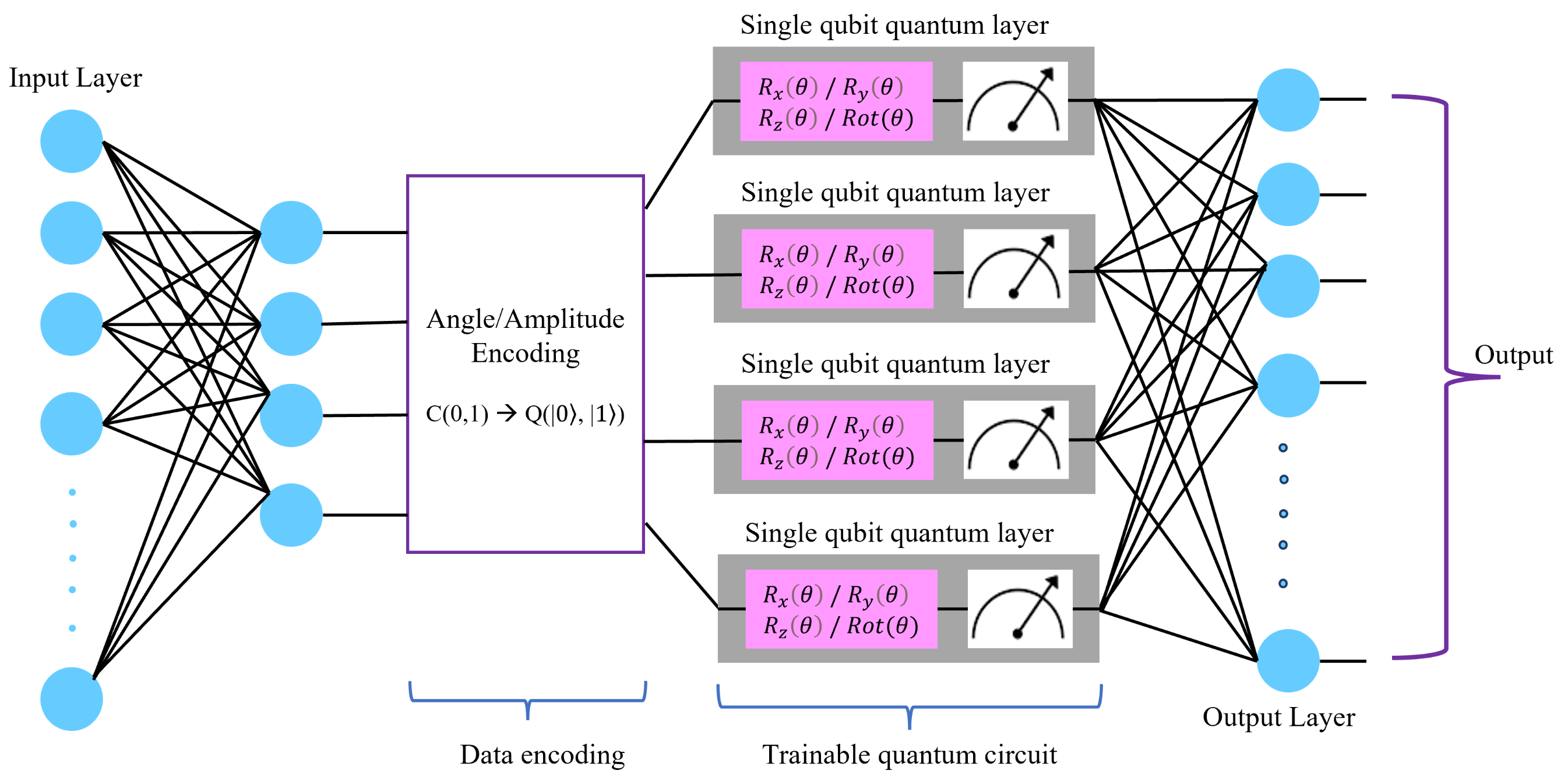
3.1. Hybrid Quantum–Classical Neural Network—Variant 1

The first variant of the implemented hybrid neural network (HQCNNv1) is relatively simple, with four qubits and only single qubit rotation gates followed by qubit measurements in the eigen-basis of σ z . The main purpose of HQCNNv1 is to (1) select the best batch sizes for the input dataset being fed to the circuit and (2) select the best parametrized rotation gates for both the data encoding techniques. Once the best parameters are selected, the rest of the hybrid network architectures is then be experimented upon to determine the best batch sizes and best gates. The complete architecture of HQCNNv1 is depicted in Figure 3.

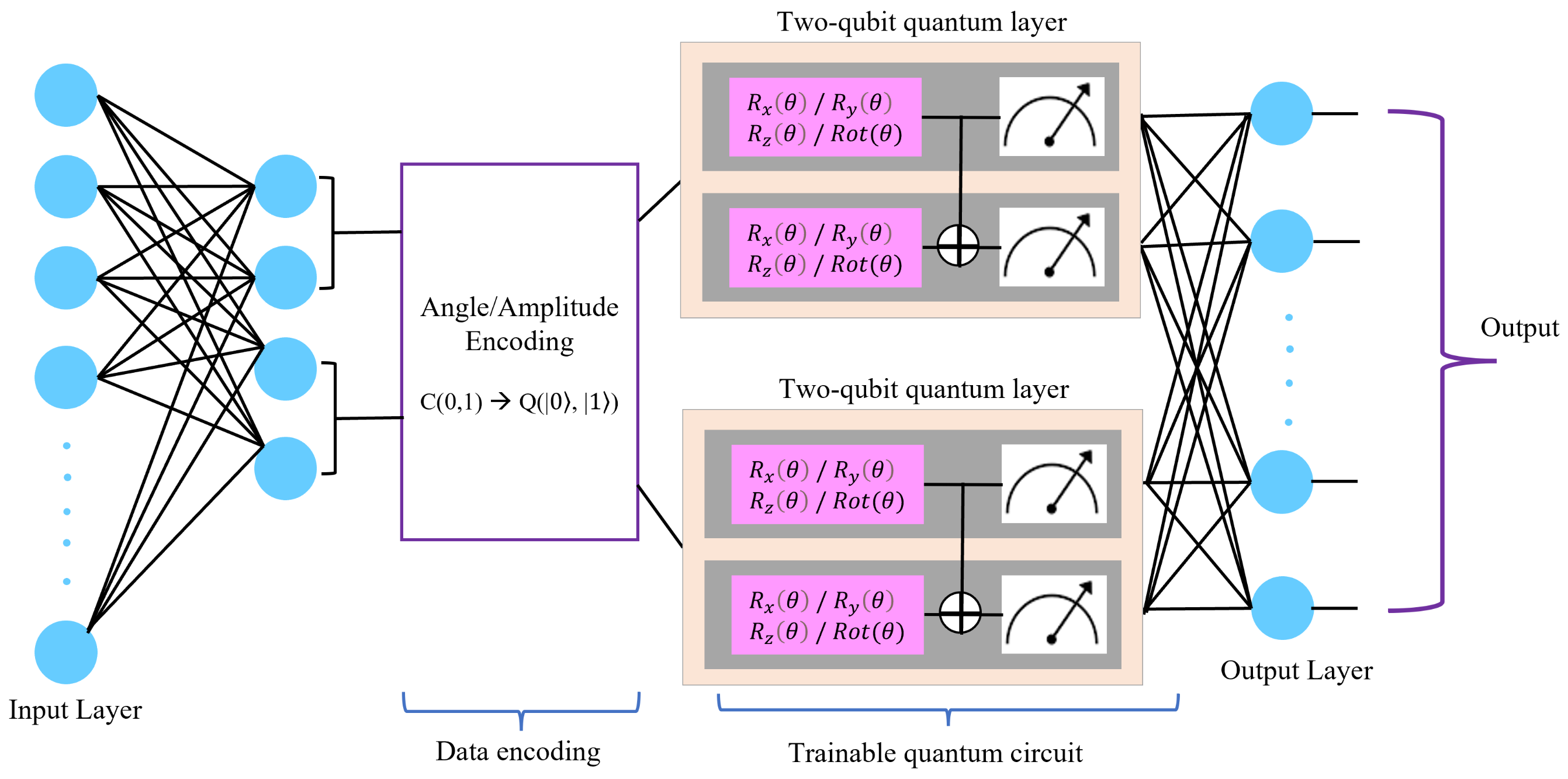
3.2. Hybrid Quantum–Classical Neural Network—Variant 2

Similar to HQCNNv1, the second variant of the hybrid network (HQCNNv2) also consists of four qubits. However, in HQCNNv2, instead of four single-qubit layers, two two-qubit layers have been used to introduce entanglement, which is one of the commonly used quantum mechanical properties in quantum computation (we use the CNOT gate create the entanglement). The HQCNNv2 architecture makes use of the best parameters (batch size and parametrized rotation gates), which we select based on the empirical results obtained for HQCNNv1 (Section 4.1). The complete architecture of HQCNNv2 is shown in Figure 4:

3.3. Hybrid Quantum–Classical Neural Network—Variant 3

In this section, we develop a more complex quantum circuit by entangling all four qubits. We analyze the performance of the third variant of the hybrid neural network (HQCNNv3) for both amplitude and angle encoding techniques with the best batch sizes and best rotation gates for each encoding (as discussed in Section 4.3. The schematic of HQCNNv3 is shown in Figure 5.

3.4. Classical Counterpart for Hybrid Networks

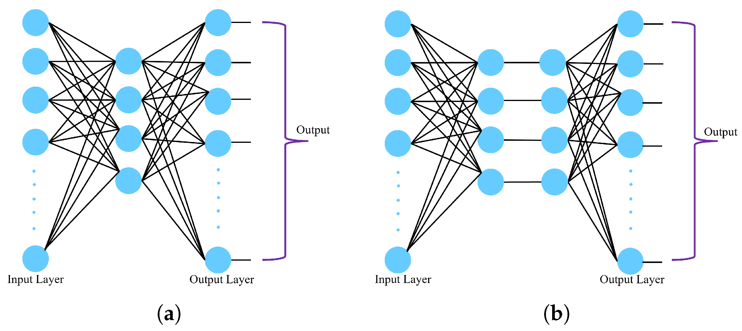
In order to compare the results and analyze the potential advantages of quantum layers in the network, we develop a pure classical model corresponding to our hybrid networks. The classical counterpart has two variants: (1) simply omitting the quantum part from Figure 3, as shown in Figure 6a, which we call CVa, and (2) replacing the four quantum layer from Figure 3 with a classical layer of four neurons, as shown in Figure 6b, which we call CVb. For a fair comparison with hybrid models, we made this classical layer a one-to-one connected layer and not a fully connected layer since the quantum layer in the hybrid network is not fully connected.

4. Results and Discussion

In this section, we report and discuss the results for all three variants of hybrid networks and two classical counterpart models for the hybrid networks.

4.1. Results—HQCNNv1

4.1.1. Small Dataset—D103

First, the HQCNNv1 was trained on D103. The following steps were performed to extract the best rotation gates and batch sizes for the small datatset:
  • The model in Figure 3 was initially trained on D103 for batch sizes of 8, 16, 32 and 64 with rotation gates R x ( θ ) , and the data were encoded via amplitude encoding. This step gave us the best batch size for D103;
  • We trained the same model with R y ( θ ) , R z ( θ ) and R o t ( θ ) gates only for the best batch sizes selected in the previous step. This step gave us the best rotation gate for amplitude encoding.
The training results for the extraction of the best batch size are presented in Table 1.
After the first step, the best batch sizes for D103 were found to be 8 and 32 with respect to accuracy, generalization and convergence time. Although the convergence time for a batch size of 64 is significantly lower than other batch sizes, it falls short in terms of overall accuracy and generalization error. The same experiment was repeated only for the best batch sizes with other rotation gates to extract the best rotation gate for amplitude encoding. The training results are presented in Table 2.
Based on the experiment results shown in Table 1 and Table 2, we can conclude that, in terms of model accuracy, all four rotation gates have comparable performance, but R y ( θ ) outperforms R x ( θ ) and R z ( θ ) in terms of model convergence time. Although R x ( θ ) is slightly better in terms of overall accuracy, its convergence time is significantly higher than R y ( θ ) . Moreover, while using R o t ( θ ) , the model converges faster, but it has reasonably low accuracy compared to the other gates, particularly R y ( θ ) . As the R y ( θ ) performs reasonably well with amplitude encoding, we use R y ( θ ) whenever we use the amplitude encoding technique in the next variants of hybrid networks.
Now, we test the same set of rotation gates for the angle encoding technique. We already have the best batch sizes for D103; therefore, we only train the model for the best batch sizes. The training results of HQCNNv1 with angle encoding are shown in Table 3.
Based on the results in Table 3, we observe that R z ( θ ) performs well with angle encoding in terms of accuracy, generalization and convergence time. Although R y ( θ ) has a relatively smaller generalization error, not only is the overall accuracy is lower, but it also takes slightly more time to converge than R z ( θ ) . Hence, R z ( θ ) is found to be the best when the data are encoded using the angle encoding technique. Therefore, we use R z ( θ ) whenever we use angle encoding in the next variants of hybrid networks.

4.1.2. Large Dataset—D204

Now, we train the same model (HQCNNv1) on D204 to analyze the change in model behavior with respect to accuracy, generalization error and convergence time. This exercise would provide grounds for a computational and expressibility (generalization ability) comparison of classical and hybrid networks by comparing the convergence rate and generalization error of both models, respectively. We use batch sizes of 8 and 32 (similar to that of D103) for fair comparison. We train the model for both amplitude and angle encoding with the corresponding best rotation gates and analyze if there is any improvement in the model performance. We observe that increasing the dataset size results in almost the same accuracy with better generalization and an obvious increase in model convergence time. The results are shown in Table 4.
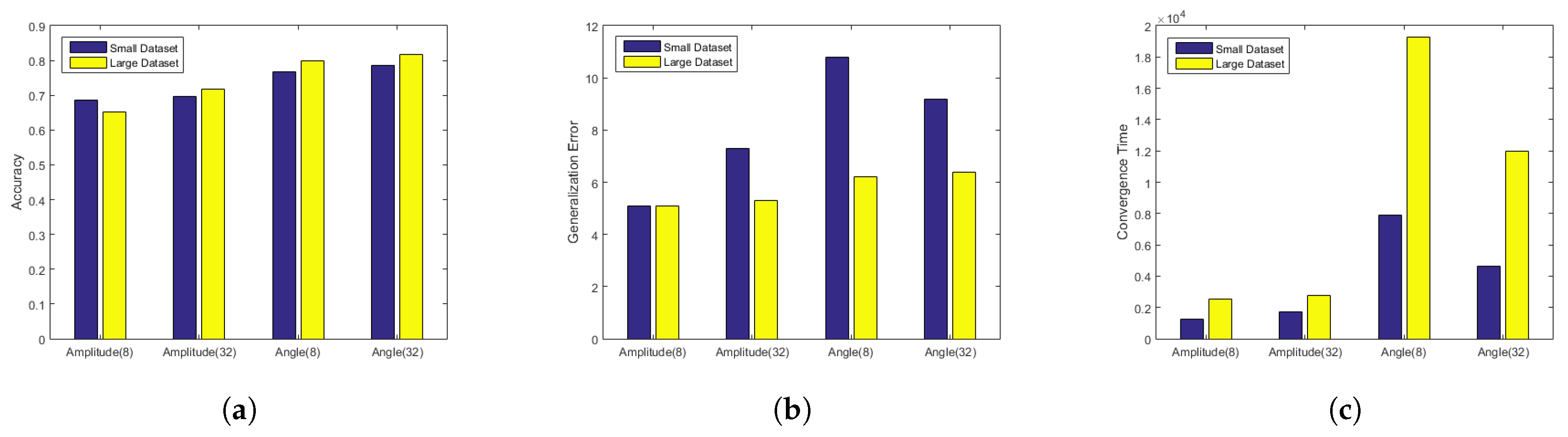
The graphical representation of the results of HQCNNv1 for both amplitude and angle encoding with the best corresponding parameters are shown in Figure 7. We observe that, analogous to classical machine learning, the hybrid (quantum–classical) approach tends to perform better with more training and testing data. The accuracy and generalization of the hybrid model improves with an increase in the dataset size, as shown in Figure 7a,b, whereas the convergence time increases (Figure 7c), which is obvious since there are more data on which to train the model. At first, angle encoding performed slightly better in terms of accuracy whereas amplitude encoding performed better in terms of generalization and convergence time.

4.2. Results—HQCNNv2

HQCNNv2, as shown in Figure 3, was implemented using the best parameters selected while experimenting with HQCNNv1. Similar to HQCNNv1, HQCNNv2 was also trained on both D103 and D204 with the best batch sizes and best rotation gates for both amplitude and angle encoding. The training results for HQCNNv2 are presented in Table 5 and visualized in Figure 8.
Like HQCNNv1, we observe that in HQCNNv2, the accuracy and generalization error tend to improve when the size of the dataset is increased, and the time of model convergence increases. Furthermore, both amplitude and angle encoding have a comparable performance with respect to overall accuracy. In addition, the amplitude encoding performed better in terms of generalization and convergence time for both D103 and D204.

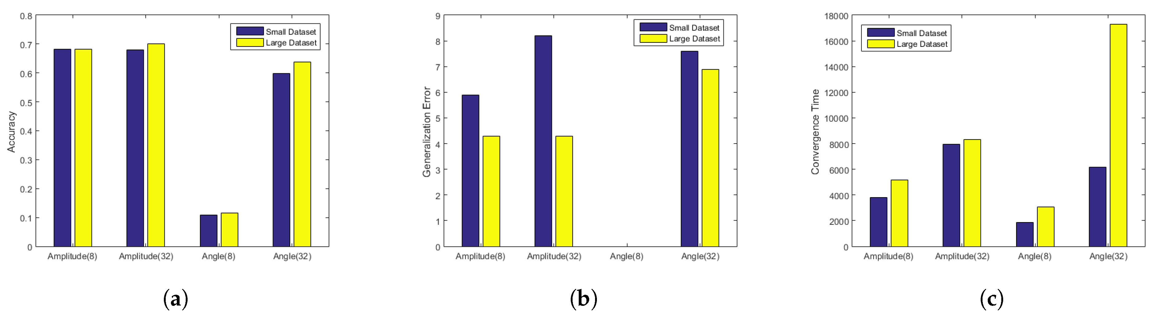
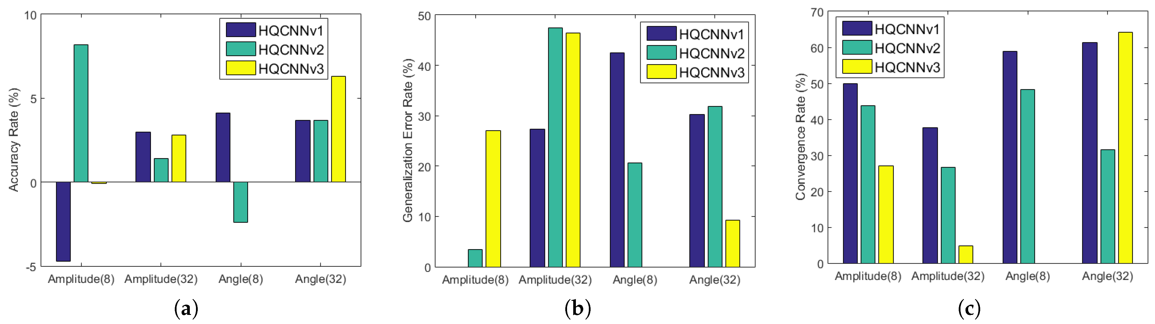
4.3. Results—HQCNNv3

The training experiment for HQCNNv3 followed the same procedure as in HQCNNv1 and HQCNNv2. The tabular and graphical representation of the obtained results for both D103 and D204 for HQCNNv3 are shown in Table 6 and Figure 9.
Similar to HQCNNv1 and HQCNNv2, when the amount of data was increased, the overall accuracy and generalization of model improved in HQCNNv3 as well, while taking more time to converge in case of larger data. Furthermore, for a smaller batch size (8), the angle encoding performed worst in HQCNNv3 with almost no learning at all (lowest accuracy). The amplitude encoding exhibited a better performance with respect to all three performance metrics (accuracy, generalization and convergence time) in HQCNNv3.

4.4. Results—CVa and CVb

We trained both classical models (CVa and CVb) on both D103 and D204 for the best batch sizes of 8 and 32. The training results for both classical models are summarized in Table 7 and visualized in Figure 10.
For D103, the classical model CVa performs slightly better than CVb in terms of convergence time, with almost the same performance in terms of accuracy and generalization. This is because CVb includes one extra hidden layer and hence tends to converge slower (particularly for a smaller batch size). For D204, both CVa and CVb have comparable accuracy. However, CVa generalizes slightly better because of its simpler architecture compared to CVb (where the latter tends to overfit).
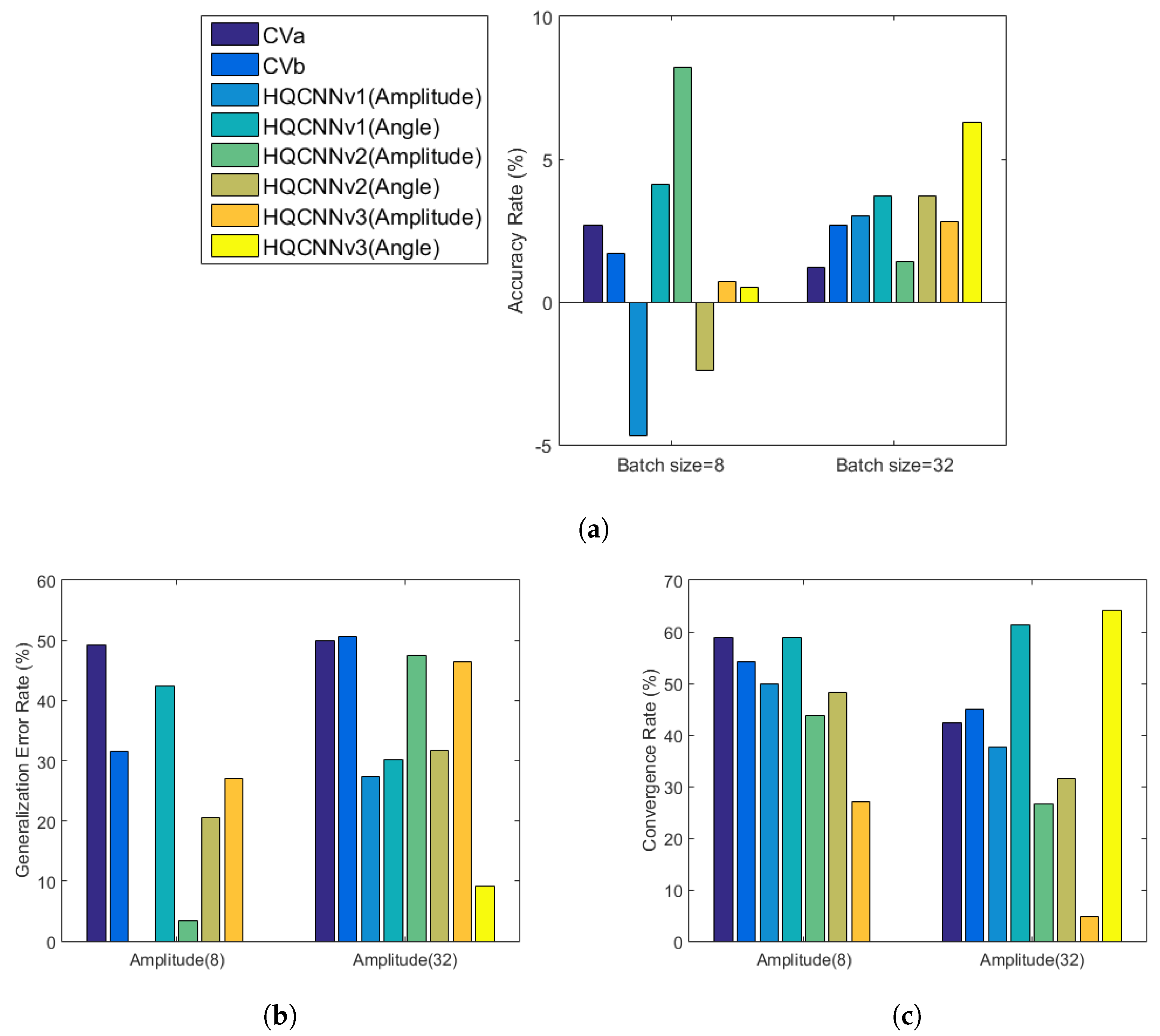
The overall performance of CVa and CVb is significantly better than HQCNNv1, particularly in terms of convergence time. This is mainly because of the classical nature of data, which can be easily encoded into the classical network. On the contrary, in hybrid networks, the classical data features are encoded into the quantum space, which is time-consuming and generally considered a bottleneck in hybrid quantum–classical algorithms. In order to demonstrate the potential quantum advantage in hybrid networks over pure classical networks, we consider the rate with which the underlying model’s performance would improve or deteriorate in terms of accuracy, generalization error and convergence time by training the networks on both D103 and 204.

5. Performance Analysis of Hybrid Networks

In this section, we compare the performance of HQCNNv1, HQCNNv2 and HQCNNv3. The performance metrics considered for the comparison are (1) accuracy, (2) generalization error and (3) the overall model convergence time. The comparison result is presented in Table 8 and Figure 11.

5.1. Accuracy

Based on the accuracy comparison results shown in column 4 of Table 8 and Figure 11a, we can conclude the following:
  • In the case of amplitude encoding and a smaller batch size, HQCNNv2 has the highest accuracy improvement rate. It is important to note here that the overall (individual) accuracy values of all the hybrid variants for smaller batch sizes are quite comparable, as already presented in their corresponding results sections;
  • For a larger batch size and amplitude encoding, all the variants have comparable individual accuracy. However, the accuracy rates of HQCNNv1 and HQCNNv3 show a comparable improvement rate, which is slightly better than HQCNNv2;
  • For angle encoding and a smaller batch size, the accuracy improvement rate is best for HQCNNv1. As the complexity of the quantum circuit increases, with angle encoding on a smaller batch size, not only does the overall (individual) accuracy tend to reduce but the accuracy improvement rate also reduces. We observe that in HQCNNv2, the accuracy improvement rate is significantly reduced, and in HQCNNv3, the model almost learns nothing and hence is not comparable in terms of accuracy improvement rate;
  • For angle encoding with a bigger batch size, the overall accuracy of all the hybrid model variants tends to reduce, but the accuracy improvement rate increases, with HQCNNv1 and HQCNNv2 having almost the same accuracy improvement rate and HQCNNv3 being slightly better.

5.2. Generalization Error

Based on the results presented in column 5 of Table 8 and Figure 11b, the following conclusions can be made regarding the generalization error of all the hybrid variants.
  • The individual generalization error values tend to reduce for all the hybrid model variants for both the encoding techniques and batch sizes when the dataset size is increased;
  • For amplitude encoding and a smaller batch size, HQCNNv3 has the highest generalization improvement rate, whereas HQCNNv1 has the worst with no improvement in generalization in the case of more data being present from which to learn;
  • For amplitude encoding and a bigger batch size, both HQCNNv2 and HQCNNv3 have a comparable generalization improvement rate that is better than HQCNNv1;
  • For angle encoding and a smaller batch size, HQCNNv1 has a better generalization improvement rate than HQCNNv2 and HQCNNv3. Since HQCNNv3 has the worst performance (almost no learning) for angle encoding with a smaller batch size, its generalization improvement rate is taken as zero;
  • For angle encoding with a bigger batch size, both HQCNNv1 and HQCNNv2 have a comparable generalization improvement rate that is better than HQCNNv3.

5.3. Convergence Time

The individual convergence time increases as increasingly complex quantum circuits are used in hybrid networks with amplitude encoding, whereas it reduces in the case of angle encoding. However, the convergence rate improves in all the scenarios. Based on the results presented in column 6 of Table 8 and Figure 11c, the following conclusions can be made regarding the convergence time of all the hybrid variants:
  • For amplitude encoding, the HQCNNv3 has the lowest increase in in convergence rate for both the batch sizes, and HQCNNv1 has the highest;
  • For angle encoding and a smaller batch size, HQCNNv2 is better than HQCNNv1. Since HQCNNv3 has the worst performance for angle encoding and a smaller batch size, we do not compare its convergence rate for other variants;
  • For angle encoding and a bigger batch size, HQCNNv2 has a better convergence rate than other variants. Moreover, the convergence rates of HQCNNv1 and HQCNNv3 are comparable.

6. Comparison of Hybrid Networks with Classical Counterparts

In this section, we perform a comparative analysis of the results obtained for all our hybrid variants and the corresponding classical counterpart models, with respect to accuracy, generalization error and convergence rate. For that purpose, we consider the rate with which the results improve or deteriorate in all the performance metrics. The comparison is presented in Table 9 and Figure 12.

6.1. Accuracy

Based on the comparison results shown in column 5 of Table 9 and Figure 12a, the following conclusions can be made:
  • For a smaller batch size, when the training and testing data are increased, the accuracy improvement rate of HQCNNv1 and HQCNNv2 is significantly better than CVa and CVb, when the data are encoded via angle and amplitude encoding, respectively. Furthermore, the overall accuracy is reduced for angle encoding in HQCNNv2 and for amplitude encoding in HQCNNv1. In addition, for a smaller batch size with angle encoding, the HQCNNv3 has the worst performance (almost no learning at all) of all the models;
  • For a bigger batch size, the accuracy improvement is better in all the hybrid models irrespective of the encoding technique, except for amplitude encoding in HQCNNv2, which can be considered as a simulator glitch.

6.2. Generalization Error Rate

Based on the comparison results shown in column 6 of Table 9 and Figure 12b, we can conclude the following:
  • When the amount of data is increased, the generalization error improvement rate for a smaller batch size is better in CVa than all the variants of hybrid models.However, it is better in HQCNNv1 than CVb and quite comparable to CVa when the data are encoded via angle encoding. Furthermore, the generalization error improvement rate in HQCNNv2 and HQCNNv3 is comparable to CVb for angle and amplitude encoding, respectively;
  • The generalization error improvement rate for a bigger batch size is also better in both classical models (CVa and CVb) than all the variants of hybrid models when we increase the training and testing data. However, the generalization improvement rate in HQCNNv2 and HQCNNv3 with amplitude encoding is comparable to CVa and CVb. Moreover, it is better in all hybrid variants for a bigger batch size when compared with smaller batch size.

6.3. Convergence Rate

Based on the comparison results shown in column 7 of Table 9 and Figure 12c, we can conclude the following:
  • For a smaller batch size, the convergence rate is better in all the hybrid networks when we increase the dataset size, except for HQCNNv1 with angle encoding, which is almost equal to that of CVa;
  • For a bigger batch size, the convergence rate of all hybrid networks is also better than CVa and CVb, except for HQCNNv1 and HQCNNv3 with angle encoding.
Since in most cases, when the size of the data is increased, we observe better convergence rates in hybrid networks compared to classical counterparts, we can say that the potential quantum advantage (computational speedup) in neural networks comes into effect.

7. Conclusions

Quantum neural networks with large quantum data and fault-tolerant quantum devices can potentially outperform classical neural networks. However, the unavailability of large-scale universal fault-tolerant quantum computers and sufficiently large quantum datasets limits their practical relevance. On the other hand, NISQ devices have already been developed and have been demonstrated to outperform classical computers for certain tasks. Hybrid quantum–classical neural networks (HQCNNs) are largely being explored for NISQ devices, where a small portion of the neural network is designed in quantum space—typically the hidden layers, sandwiched between classical input and output layers. Using classical data, HQCNNs attempt to leverage the quantum advantage in neural networks. However, it is still not proven that HQCNNs have an advantage over classical NNs (particularly for classical data).
Realizing the lack of a standardized methodology to design quantum layers in HQCNN, in this work, we propose a systematic methodology to construct these quantum layers. Such quantum layers are typically constructed using variational or parametrized quantum circuits. However, before running the quantum layer, the classical data need to be encoded, which is the most important step in HQCNNs and is often considered the performance bottleneck. In this paper, we use two of the most commonly used encoding techniques, namely amplitude and angle encoding.
We propose three variants of HQCNNs. HQCNNv1 consists of four single-qubit layers and is tested with all commonly used parametrized gates and both the encodings. We conclude that for amplitude encoding, R y ( θ ) performs the best, whereas R z ( θ ) is best to use with angle encoding, with respect to our performance metrics (accuracy, generalization and convergence time). HQCNNv2 and HQCNNv3 introduce fairly complex and reasonably complex entanglement, respectively.
We then compare all three hybrid variants, for which we consider the overall rate at which each performance metric improves or deteriorates when we increase the data, since we believe that quantum advantages are clearer with more computational data.
The results of the comparison of the hybrid variants do not lead to a single winner that is an optimal choice for all the scenarios and applications. Hence, considering any of the variants is highly application-dependent. An overview of variants’ selection preference for some applications is presented in Table 10. For instance, healthcare applications usually require higher accuracy, and thus HQCNNv1 would be more appropriate choice. Similarly, applications such as recommendation systems can accommodate relatively low accuracy for faster model convergence, in which case HQCNNv3 would be a preferred variant. Finally, both HQCNNv2 and HQCNNv3 can be a desirable choice for applications in which accuracy and convergence need to be balanced, such as facial and speech recognition applications.
When evaluating the encoding techniques, we conclude that amplitude encoding is significantly faster than angle encoding, mainly because it encodes an exponential amount of data for n number of qubits, whereas angle encoding is slightly better in terms of overall accuracy, particularly for simple quantum circuits. Hence, amplitude encoding is recommended for applications where convergence time is the most important metric and angle encoding where accuracy is most important.
We also compare our hybrid variants with two distinct variants of classical counterparts. We observed that the accuracy improvement rate and model convergence are better in all hybrid variants for the majority of the experiments, and hence it is safe to say that when the amount of data is increased, the potential quantum advantages start to enhance the performance rate of HQCNNs as compared to pure classical NNs. Although the classical models generalize slightly better than hybrid variants, the generalization improvement rate of hybrid variants is still quite comparable to classical models.

Author Contributions

Conceptualization, M.K. and S.A.-K.; methodology, M.K and S.A.-K.; software, M.K.; validation, M.K. and S.A.-K.; formal analysis, M.K.; investigation, M.K.; resources, M.K.; data curation, M.K.; writing—original draft preparation, M.K.; writing—review and editing, M.K. and S.A.-K.; visualization, M.K.; supervision, S.A.-K.; project administration, S.A.-K.; funding acquisition, S.A.-K. All authors have read and agreed to the published variant of the manuscript.

Funding

This research received no external funding.

Institutional Review Board Statement

Not applicable.

Informed Consent Statement

Not applicable.

Data Availability Statement

The data used for training purposes were taken from the MNIST dataset, which can be found at http://yann.lecun.com/exdb/mnist/.

Conflicts of Interest

The authors declare no conflict of interest.

Abbreviations

The following abbreviations are used in this manuscript:
NNsNeural networks
QNNsQuantum neural networks
HQCNNsHybrid quantum–classical neural networks
DSEDesign space exploration
D103Small dataset
D204Large dataset
HQCNNv1First variant hybrid quantum–classical neural network
HQCNNv2Second variant hybrid quantum–classical neural network
HQCNNv3Third variant hybrid quantum–classical neural network
CVaFirst variant of classical counterpart
CVbSecond variant of classical counterpart

References

  1. Sarker, I.H. Machine Learning: Algorithms, Real-World Applications and Research Directions. SN Comput. Sci. 2021, 2, 2661–8907. [Google Scholar] [CrossRef]
  2. Maind, S.B.; Wankar, P. Research paper on basic of artificial neural network. Int. J. Recent Innov. Trends Comput. Commun. 2014, 2, 96–100. [Google Scholar]
  3. Najafabadi, M.M.; Villanustre, F.; Khoshgoftaar, T.M.; Seliya, N.; Wald, R.; Muharemagic, E. Deep learning applications and challenges in big data analytics. J. Big Data 2015, 2, 1–21. [Google Scholar] [CrossRef] [Green Version]
  4. Hinton, G.; Deng, L.; Yu, D.; Dahl, G.E.; Mohamed, A.R.; Jaitly, N.; Senior, A.; Vanhoucke, V.; Nguyen, P.; Sainath, T.N.; et al. Deep Neural Networks for Acoustic Modeling in Speech Recognition: The Shared Views of Four Research Groups. IEEE Signal Process. Mag. 2012, 29, 82–97. [Google Scholar] [CrossRef]
  5. Seide, F.; Li, G.; Yu, D. Conversational speech transcription using context-dependent deep neural networks. In Proceedings of the Twelfth Annual Conference of the International Speech Communication Association, Florence, Italy, 27–31 August 2011. [Google Scholar]
  6. Andina, D.; Voulodimos, A.; Doulamis, N.; Doulamis, A.; Protopapadakis, E. Deep Learning for Computer Vision: A Brief Review. Comput. Intell. Neurosci. 2018, 18, 1687–5265. [Google Scholar] [CrossRef]
  7. Krizhevsky, A.; Sutskever, I.; Hinton, G.E. Imagenet classification with deep convolutional neural networks. Adv. Neural Inf. Process. Syst. 2012, 25, 1097–1105. [Google Scholar] [CrossRef]
  8. Mikolov, T.; Deoras, A.; Kombrink, S.; Burget, L.; Cernocký, J. Empirical Evaluation and Combination of Advanced Language Modeling Techniques; INTERSPEECH. ISCA: Incheon, Korea, 2011; pp. 605–608. [Google Scholar]
  9. Tuor, A.; Kaplan, S.; Hutchinson, B.; Nichols, N.; Robinson, S. Deep Learning for Unsupervised Insider Threat Detection in Structured Cybersecurity Data Streams. arXiv 2017, arXiv:cs.NE/1710.00811. [Google Scholar]
  10. Nasser, I.M.; Abu-Naser, S.S. Lung cancer detection using artificial neural network. Int. J. Eng. Inf. Syst. (IJEAIS) 2019, 3, 17–23. [Google Scholar]
  11. Shahid, N.; Rappon, T.; Berta, W. Applications of artificial neural networks in health care organizational decision-making: A scoping review. PLoS ONE 2019, 14, e0212356. [Google Scholar]
  12. Goodfellow, I.; Bengio, Y.; Courville, A. Deep Learning; MIT Press: Cambridge, MA, USA, 2016; Available online: http://www.deeplearningbook.org (accessed on 3 October 2021).
  13. Vapnik, V. The Nature of Statistical Learning Theory; Springer Science & Business Media: New York, NY, USA, 2013. [Google Scholar]
  14. Mohri, M.; Rostamizadeh, A.; Talwalkar, A. Foundations of Machine Learning; MIT Press: Cambridge, MA, USA, 2018. [Google Scholar]
  15. Barbiero, P.; Squillero, G.; Tonda, A. Modeling Generalization in Machine Learning: A Methodological and Computational Study. arXiv 2020, arXiv:cs.LG/2006.15680. [Google Scholar]
  16. Arute, F.; Arya, K.; Babbush, R.; Bacon, D.; Bardin, J.C.; Barends, R.; Biswas, R.; Boixo, S.; Brandao, F.G.S.L.; Buell, D.A.; et al. Quantum supremacy using a programmable superconducting processor. Nature 2019, 574, 505–510. [Google Scholar] [CrossRef] [Green Version]
  17. Zhong, H.S.; Wang, H.; Deng, Y.H.; Chen, M.C.; Peng, L.C.; Luo, Y.H.; Qin, J.; Wu, D.; Ding, X.; Hu, Y.; et al. Quantum computational advantage using photons. Science 2020, 370, 1460–1463. [Google Scholar] [CrossRef] [PubMed]
  18. Wu, Y.; Bao, W.S.; Cao, S.; Chen, F.; Chen, M.C.; Chen, X.; Chung, T.H.; Deng, H.; Du, Y.; Fan, D.; et al. Strong quantum computational advantage using a superconducting quantum processor. arXiv 2021, arXiv:quant-ph/2106.14734. [Google Scholar] [CrossRef]
  19. McGeoch, C.C. Adiabatic quantum computation and quantum annealing: Theory and practice. Synth. Lect. Quantum Comput. 2014, 5, 1–93. [Google Scholar] [CrossRef]
  20. Hauke, P.; Katzgraber, H.; Lechner, W.; Nishimori, H.; Oliver, W. Perspectives of quantum annealing: Methods and implementations. Rep. Prog. Phys. 2020, 83, 054401. [Google Scholar] [CrossRef] [PubMed] [Green Version]
  21. Schuld, M.; Sinayskiy, I.; Petruccione, F. The quest for a Quantum Neural Network. Quantum Inf. Process. 2014, 13, 2567–2586. [Google Scholar] [CrossRef] [Green Version]
  22. Biamonte, J.; Wittek, P.; Pancotti, N.; Rebentrost, P.; Wiebe, N.; Lloyd, S. Quantum machine learning. Nature 2017, 549, 195–202. [Google Scholar] [CrossRef]
  23. Havlíček, V.; Córcoles, A.D.; Temme, K.; Harrow, A.W.; Kandala, A.; Chow, J.M.; Gambetta, J.M. Supervised learning with quantum-enhanced feature spaces. Nature 2019, 567, 209–212. [Google Scholar] [CrossRef] [Green Version]
  24. Cerezo, M.; Arrasmith, A.; Babbush, R.; Benjamin, S.C.; Endo, S.; Fujii, K.; McClean, J.R.; Mitarai, K.; Yuan, X.; Cincio, L.; et al. Variational Quantum Algorithms. arXiv 2020, arXiv:quant-ph/2012.09265. [Google Scholar] [CrossRef]
  25. Farhi, E.; Neven, H. Classification with Quantum Neural Networks on Near Term Processors. arXiv 2018, arXiv:quant-ph/1802.06002. [Google Scholar]
  26. Mitarai, K.; Negoro, M.; Kitagawa, M.; Fujii, K. Quantum circuit learning. Phys. Rev. A 2018, 98, 032309. [Google Scholar] [CrossRef] [Green Version]
  27. Kandala, A.; Mezzacapo, A.; Temme, K.; Takita, M.; Brink, M.; Chow, J.M.; Gambetta, J.M. Hardware-efficient variational quantum eigensolver for small molecules and quantum magnets. Nature 2017, 549, 242–246. [Google Scholar] [CrossRef] [PubMed]
  28. Hempel, C.; Maier, C.; Romero, J.; McClean, J.; Monz, T.; Shen, H.; Jurcevic, P.; Lanyon, B.P.; Love, P.; Babbush, R.; et al. Quantum Chemistry Calculations on a Trapped-Ion Quantum Simulator. Phys. Rev. X 2018, 8, 031022. [Google Scholar] [CrossRef] [Green Version]
  29. Arute, F.; Arya, K.; Babbush, R.; Bacon, D.; Bardin, J.C.; Barends, R.; Boixo, S.; Broughton, M.; Buckley, B.B.; Buell, D.A.; et al. Hartree-Fock on a superconducting qubit quantum computer. Science 2020, 369, 1084–1089. [Google Scholar] [CrossRef]
  30. Cong, I.; Choi, S.; Lukin, M.D. Quantum convolutional neural networks. Nat. Phys. 2019, 15, 1273–1278. [Google Scholar] [CrossRef] [Green Version]
  31. Beer, K.; Bondarenko, D.; Farrelly, T.; Osborne, T.J.; Salzmann, R.; Scheiermann, D.; Wolf, R. Training deep quantum neural networks. Nat. Commun. 2020, 11, 1–6. [Google Scholar] [CrossRef] [PubMed] [Green Version]
  32. Du, Y.; Hsieh, M.H.; Liu, T.; Tao, D. A Grover-search based quantum learning scheme for classification. New J. Phys. 2021, 23, 023020. [Google Scholar] [CrossRef]
  33. Zhu, D.; Linke, N.M.; Benedetti, M.; Landsman, K.A.; Nguyen, N.H.; Alderete, C.H.; Perdomo-Ortiz, A.; Korda, N.; Garfoot, A.; Brecque, C.; et al. Training of quantum circuits on a hybrid quantum computer. Sci. Adv. 2019, 5, 9918. [Google Scholar] [CrossRef] [PubMed] [Green Version]
  34. Rudolph, M.S.; Toussaint, N.B.; Katabarwa, A.; Johri, S.; Peropadre, B.; Perdomo-Ortiz, A. Generation of High-Resolution Handwritten Digits with an Ion-Trap Quantum Computer. arXiv 2020, arXiv:quant-ph/2012.03924. [Google Scholar]
  35. Huang, H.L.; Du, Y.; Gong, M.; Zhao, Y.; Wu, Y.; Wang, C.; Li, S.; Liang, F.; Lin, J.; Xu, Y.; et al. Experimental Quantum Generative Adversarial Networks for Image Generation. Phys. Rev. Appl. 2021, 16, 024051. [Google Scholar] [CrossRef]
  36. Du, Y.; Hsieh, M.H.; Liu, T.; You, S.; Tao, D. On the learnability of quantum neural networks. arXiv 2020, arXiv:quant-ph/2007.12369. [Google Scholar] [CrossRef]
  37. Banchi, L.; Pereira, J.; Pirandola, S. Generalization in Quantum Machine Learning: A Quantum Information Perspective. arXiv 2021, arXiv:quant-ph/2102.08991. [Google Scholar]
  38. Huang, H.Y.; Broughton, M.; Mohseni, M.; Babbush, R.; Boixo, S.; Neven, H.; McClean, J.R. Power of data in quantum machine learning. Nat. Commun. 2021, 12, 1–9. [Google Scholar] [CrossRef] [PubMed]
  39. Abbas, A.; Sutter, D.; Zoufal, C.; Lucchi, A.; Figalli, A.; Woerner, S. The power of quantum neural networks. Nat. Comput. Sci. 2021, 1, 403–409. [Google Scholar] [CrossRef]
  40. Bu, K.; Koh, D.E.; Li, L.; Luo, Q.; Zhang, Y. On the statistical complexity of quantum circuits. arXiv 2021, arXiv:quant-ph/2101.06154. [Google Scholar]
  41. Du, Y.; Tu, Z.; Yuan, X.; Tao, D. An efficient measure for the expressivity of variational quantum algorithms. arXiv 2021, arXiv:quant-ph/2104.09961. [Google Scholar]
  42. Huang, H.Y.; Kueng, R.; Preskill, J. Information-Theoretic Bounds on Quantum Advantage in Machine Learning. Phys. Rev. Lett. 2021, 126, 190505. [Google Scholar] [CrossRef] [PubMed]
  43. Qian, Y.; Wang, X.; Du, Y.; Wu, X.; Tao, D. The dilemma of quantum neural networks. arXiv 2021, arXiv:quant-ph/2106.04975. [Google Scholar]
  44. LeCun, Y. The MNIST Database of Handwritten Digits. 1998. Available online: http://yann.lecun.com/exdb/mnist/ (accessed on 16 September 2021).
  45. Verdon, G.; Broughton, M.; McClean, J.R.; Sung, K.J.; Babbush, R.; Jiang, Z.; Neven, H.; Mohseni, M. Learning to learn with quantum neural networks via classical neural networks. arXiv 2019, arXiv:quant-ph/1907.05415. [Google Scholar]
  46. Liang, Y.; Peng, W.; Zheng, Z.J.; Silvén, O.; Zhao, G. A hybrid quantum-classical neural network with deep residual learning. arXiv 2021, arXiv:cs.LG/2012.07772. [Google Scholar] [CrossRef] [PubMed]
  47. Beer, K.; List, D.; Müller, G.; Osborne, T.J.; Struckmann, C. Training Quantum Neural Networks on NISQ Devices. arXiv 2021, arXiv:quant-ph/2104.06081. [Google Scholar]
  48. Wei, S.; Chen, Y.; Zhou, Z.; Long, G. A Quantum Convolutional Neural Network on NISQ Devices. arXiv 2021, arXiv:quant-ph/2104.06918. [Google Scholar]
  49. McClean, J.R.; Boixo, S.; Smelyanskiy, V.N.; Babbush, R.; Neven, H. Barren plateaus in quantum neural network training landscapes. Nat. Commun. 2018, 9, 1–6. [Google Scholar] [CrossRef] [Green Version]
  50. Pesah, A.; Cerezo, M.; Wang, S.; Volkoff, T.; Sornborger, A.T.; Coles, P.J. Absence of Barren Plateaus in Quantum Convolutional Neural Networks. Phys. Rev. X 2021, 11, 041011. [Google Scholar] [CrossRef]
  51. Patti, T.L.; Najafi, K.; Gao, X.; Yelin, S.F. Entanglement devised barren plateau mitigation. Phys. Rev. Res. 2021, 3, 033090. [Google Scholar] [CrossRef]
  52. LaRose, R.; Coyle, B. Robust data encodings for quantum classifiers. Phys. Rev. A 2020, 102, 032420. [Google Scholar] [CrossRef]
  53. Schuld, M.; Petruccione, F. Supervised Learning with Quantum Computers; Springer: Berlin/Heidelberg, Germany, 2018; Volume 17. [Google Scholar]
  54. Cao, S.; Wossnig, L.; Vlastakis, B.; Leek, P.; Grant, E. Cost-function embedding and dataset encoding for machine learning with parametrized quantum circuits. Phys. Rev. A 2020, 101, 052309. [Google Scholar] [CrossRef]
  55. Grant, E.; Benedetti, M.; Cao, S.; Hallam, A.; Lockhart, J.; Stojevic, V.; Green, A.G.; Severini, S. Hierarchical quantum classifiers. NPJ Quantum Inf. 2018, 4, 1–8. [Google Scholar] [CrossRef] [Green Version]
  56. Stoudenmire, E.M.; Schwab, D.J. Supervised learning with quantum-inspired tensor networks. arXiv 2016, arXiv:1605.05775. [Google Scholar]
  57. Benedetti, M.; Realpe-Gómez, J.; Perdomo-Ortiz, A. Quantum-assisted Helmholtz machines: A quantum–classical deep learning framework for industrial datasets in near-term devices. Quantum Sci. Technol. 2018, 3, 034007. [Google Scholar] [CrossRef] [Green Version]
Figure 1. Quantum neural network architecture. U ( x ) is a set of unitary operations dependent on input data and responsible for encoding input data into quantum devices. V ( θ ) is the variational quantum circuit consisting of a set of parametrized gates, which depends on trainable parameters θ . When the circuit is measured, it is classically post-processed and interpreted as a prediction ( y ^ ) of QNN.
Electronics 10 02980 g001
Figure 2. Typical architecture of hybrid quantum–classical neural network (HQCNN) architecture.
Electronics 10 02980 g002
Figure 3. Schematic of variant 1 of hybrid quantum–classical neural network architecture.
Electronics 10 02980 g003
Figure 4. Schematic of variant 2 of hybrid quantum–classical neural network architecture.
Electronics 10 02980 g004
Figure 5. Schematic of variant 3 of hybrid quantum–classical neural network architecture.
Electronics 10 02980 g005
Figure 6. Classical counterparts for hybrid networks. (a) First variant of classical counterpart (CVa); (b) Second variant of classical counterpart (CVb).
Electronics 10 02980 g006
Figure 7. HQCNNv1 results for D103 and D204. (a) Accuracy, (b) generalization error, (c) convergence time. The values on the x-axis denote the encoding technique, with corresponding batch sizes in parentheses.
Electronics 10 02980 g007
Figure 8. HQCNNv2 results for both D103 and D204. (a) Accuracy, (b) generalization error, (c) convergence time. The values on the x-axis denote the encoding technique with corresponding batch sizes in parentheses.
Electronics 10 02980 g008
Figure 9. HQCNNv3 results for both D103 and D204. (a) Accuracy, (b) generalization error, (c) convergence time. The x-axis represents the encoding technique with corresponding batch size in parentheses.
Electronics 10 02980 g009
Figure 10. Results of CVa and CVb. (a) Accuracy rate comparison, (b) generalization error rate comparison, (c) convergence rate comparison. The x-axis represents the classical model variant with the corresponding batch size in parentheses.
Electronics 10 02980 g010
Figure 11. Comparison of HQCNNv1, HQCNNv2, HQCNNv3. (a) Accuracy rate (b) generalization error rate, (c) convergence rate. The x-axis represents the encoding technique with corresponding batch sizes in parentheses.
Electronics 10 02980 g011
Figure 12. Comparison of all hybrid variants with classical counterparts. (a) Accuracy rate, (b) generalization error rate, (c) convergence rate.
Electronics 10 02980 g012
Table 1. HQCNNv1 training results with amplitude encoding for D103.
Batch SizeRotation GateMaximum Train AccuracyMaximum Validation AccuracyGeneralization ErrorConvergence Time (s)
8 R x ( θ ) 0.74230.69424.87250.72
16 R x ( θ ) 0.75820.67508.36669.1
32 R x ( θ ) 0.80820.72907.96500.5
64 R x ( θ ) 0.76080.66879.24147.7
Table 2. HQCNNv1 training results for best batch size with amplitude encoding for D103.
Batch SizeRotation GateMaximum Train AccuracyMaximum Validation AccuracyGeneralization ErrorConvergence Time (s)
8 R y ( θ ) 0.73670.68505.11274.8
32 R y ( θ ) 0.76930.69607.31741.07
8 R z ( θ ) 0.76600.68707.95213.11
32 R z ( θ ) 0.74630.65279.34867.32
8 R o t ( θ ) 0.70920.64376.61775.5
32 R o t ( θ ) 0.62940.59333.61527.5
Table 3. HQCNNv1 training results with angle encoding for D103.
Batch SizeRotation GateMaximum Train AccuracyMaximum Validation AccuracyGeneralization ErrorConvergence Time (s)
8 R x ( θ ) 0.89140.787010.449681.8
32 R x ( θ ) 0.89170.783710.87133.7
8 R y ( θ ) 0.74790.629011.98339.2
32 R y ( θ ) 0.88150.79678.45511.7
8 R z ( θ ) 0.87440.766310.87929.13
32 R z ( θ ) 0.87870.78709.174637.33
8 R o t ( θ ) 0.86950.746712.2810427.7
32 R o t ( θ ) 0.89010.770711.948985.01
Table 4. HQCNNv1 training results with both encodings for D204.
EncodingBatch SizeRotation GateMaximum Train AccuracyMaximum Validation AccuracyGeneralization ErrorConvergence Time (s)
Amplitude8 R y ( θ ) 0.70410.65255.12544.8
Amplitude32 R y ( θ ) 0.77060.71755.32794.8
Angle8 R z ( θ ) 0.86220.79936.210,248.4
Angle32 R z ( θ ) 0.88160.81756.412,003.4
Table 5. HQCNNv2 training results on D103 and D204 with both encodings.
EncodingBatch SizeRotation GateMaximum Train AccuracyMaximum Validation AccuracyGeneralization ErrorConvergence Time (s)
Small Dataset—D103
Amplitude8 R y ( θ ) 0.74820.69035.83649.4
Amplitude32 R y ( θ ) 0.76900.68678.23649.4
Angle8 R z ( θ ) 0.78860.69179.76662.6
Angle32 R z ( θ ) 0.83450.728010.76262.4
Large Dataset—D204
Amplitude8 R y ( θ ) 0.79290.75254.046493.9
Amplitude32 R y ( θ ) 0.73950.69704.35823.8
Angle8 R z ( θ ) 0.75230.67557.712679.1
Angle32 R z ( θ ) 0.82910.75637.39152.6
Table 6. HQCNNv3 training results for D103 and D204 with both encodings.
EncodingBatch SizeRotation GateMaximum Train AccuracyMaximum Validation AccuracyGeneralization ErrorConvergence Time (s)
Small Dataset—D103
Amplitude8 R y ( θ ) 0.74060.68175.93780.7
Amplitude32 R y ( θ ) 0.74490.68005.67941.9
Angle8 R z ( θ ) 0.10800.1087∼01879.6
Angle32 R z ( θ ) 0.67450.59837.66184.2
Large Dataset—D204
Amplitude8 R y ( θ ) 0.72830.68124.35178.6
Amplitude32 R y ( θ ) 0.72970.69983.08341.5
Angle8 R z ( θ ) 0.11330.1145∼03046.5
Angle32 R z ( θ ) 0.70780.63906.917,304.1
Table 7. Training results of both classical counterpart models on both D103 and D204.
Batch SizeClassical Model VariantMaximum Train AccuracyMaximum Validation AccuracyGeneralization ErrorConvergence Time (s)
Small Dataset—D103
8CVa0.89370.82037.37.54
32CVa0.90310.82477.84.67
Large Dataset—D204
8CVa0.88110.84353.724.21
32CVa0.87450.83503.98.09
Small Dataset—D103
8CVb0.90530.82877.313.19
32CVb0.89480.81977.54.82
Large Dataset—D204
8CVb0.89370.84375.028.8
32CVb0.88020.84283.78.78
Table 8. Comparison of all hybrid network variants.
EncodingBatch SizeModel VariantImproved Accuracy Rate (%)Improved Generalization Error Rate (%)Increase in Convergence Rate (%)
Amplitude8HQCNNv1−4.7∼049.9
Amplitude32HQCNNv13.027.337.7
Angle8HQCNNv14.142.558.8
Angle32HQCNNv13.730.261.4
Amplitude8HQCNNv28.23.443.8
Amplitude32HQCNNv21.447.526.7
Angle8HQCNNv2−2.420.648.2
Angle32HQCNNv23.731.831.5
Amplitude8HQCNNv30.0727.127.0
Amplitude32HQCNNv32.846.44.8
Angle8HQCNNv3worstworstworst
Angle32HQCNNv36.39.264.2
Table 9. Comparison of classical and hybrid network variants.
ModelVariantEncodingBatch SizeImproved Accuracy Rate (%)Improved Generalization Error Rate (%)Increase in Convergence Rate (%)
ClassicalCVa-82.749.358.9
ClassicalCVa-321.250.042.3
ClassicalCVb-81.731.554.2
ClassicalCVb-322.750.645.1
HybridHQCNNv1Amplitude8−4.7049.9
323.027.337.7
Angle84.142.558.8
323.730.261.4
HybridHQCNNv2Amplitude88.23.443.8
321.447.526.7
Angle8−2.420.648.2
323.731.831.5
HybridHQCNNv3Amplitude80.0727.127.0
322.846.44.8
Angle8∼0∼0∼0
326.39.264.2
Table 10. Variant selection for respective application requirements.
ObjectiveHQCNNv1HQCNNv2HQCNNv3
High Accuracy312
Better Generalization312
Fast Convergence321
1: First Preference, 2: Second Preference, 3: Third Preference.
Publisher’s Note: MDPI stays neutral with regard to jurisdictional claims in published maps and institutional affiliations.

