1. Introduction
The ongoing technological developments and the expansion of the Internet of Things have led to an overwhelming amount of data being collected in real time by a wide range of sensors and end devices, such as smartphones. This raises the need for the real-time processing of data using AI in order to perform knowledge extraction and transform the data into meaningful information which can be acted upon. Hence, yesterday’s sensors and embedded computing devices are transcending into today’s edge computing nodes, with the aim of processing the data as close to the originating source as possible.
The most powerful machine learning technology used today for data processing and analysis is deep earning, which has been shown to be successful in a variety of application domains ranging from computer vision [
1] and human activity recognition [
2] to natural language processing [
3] and others. The concept of edge intelligence—running deep learning on edge devices—has the potential to ameliorate several drawbacks associated with traditional centralized computing, among which are network latency, scalability, privacy and data security concerns.
However, several important challenges hinder the performance of deep learning at the edge. High accuracy and high resource consumption are defining characteristics of deep learning, which inherently come into conflict with the resource-constrained nature and (as in the cases of smartphones) limited battery capacity of edge computing devices. To achieve high accuracy, a DNN (deep neural network) requires significant amounts of memory to store all the model parameters and will have a high latency because of all the matrix multiplications being performed. In addition, Graphics Processing Units (GPUs) play a critical role in efficient DNN inference and training. Some of the most widely used GPU software libraries, such as CUDA [
4] and cuDNN [
5] (which is targeted towards deep learning), are not widely available on many edge computing nodes such as today’s smartphones [
6].
The last decade’s research efforts have begun to question the necessity of such a large number of parameters and network layers in deep learning models [
7]. Consequently, focus has shifted towards reducing the computational complexity of deep learning models through several design strategies, such as knowledge distillation [
8], early exit [
9] and network compression [
10]. Nevertheless, all such neural network complexity reduction methods come with the downside of decreasing inference accuracy as the network compression rate increases. In addition, traditional approaches apply a single static compression to the network, which then operates in a permanently impaired state regardless of any changes in circumstances that may arise and call for a more or less accurate network inference.
Recent advances mitigate this issue by proposing adaptive compression techniques that can dynamically adjust the network compression rate during runtime. These approaches, such as Slimmable Neural Networks [
11] or Any-Precision Deep Neural Networks [
12], promise to facilitate the flexible deployment of deep learning models in scenarios where a trade-off between inference accuracy and runtime efficiency are sought. These approaches enable the on-demand engagement of fewer or more deep learning parameters, or an on-demand usage of a lower or a higher numerical precision, and thus balance the precision and the execution speedup. To date, however, these approaches have only been examined at a very high level, and their practical utility in real-world applications and on actual edge devices is unexplored. Moreover, while the above approaches, at least theoretically, enable an accuracy–resource usage trade-off, it remains unclear how to dynamically adapt the operation along the trade-off line in order to maximize the achieved accuracy with minimal resource usage.
In this paper, inspired by the Approximate Mobile Computing principles [
13], we propose an innovative approach for dynamic mobile deep learning adaptation that aims to bridge the gap between the theoretical resource savings brought by adaptive neural network compression techniques and the requirements of a real-world mobile application. We devise original algorithms that continuously analyze the difficulty of the inference task and for each input dynamically guide the neural network compression rate in a mobile human activity recognition scenario. Our approach has the potential to foster the deployment of deep learning on resource-constrained IoT edge devices by enabling neural networks to scale their resource usage and thus energy consumption, according to the environmental factors and context of use, with tolerable accuracy drops.
The main contributions of this work are summarized as follows:
We investigate the inference accuracy and the energy saving potential as well as the practicality of two orthogonal neural network compression techniques (quantization and slimming) in the context of mobile human activity recognition;
We devise dynamic neural network compression adaptation algorithms that achieve a comparable inference accuracy with up to 33% fewer network parameters compared to the best-performing static compression;
We conduct a 21-person experiment and assess the utility of our deep learning adaptation approach on a previously unseen dataset, while also demonstrating the real-world usability of the implementation and the potential of real-world energy savings it brings.
Given that one of the main challenges in machine learning-related research is to ensure that the presented and published results are sound and reliable, we performed our research with reproducibility in mind [
14], and we have made the code and collected experimental data publicly available to the research community at:
https://gitlab.fri.uni-lj.si/lrk/mobilenn-slimming-and-quantization (accessed on 4 November 2021).
4. Dynamic Neural Network Adaptation Algorithms
The techniques described in
Section 3.1 provide a means for trading off accuracy for reduced resource usage; however, none of the techniques prescribes the manner in which the adaptation should be performed in order to achieve a particular target accuracy or, in accordance to the goals of our work, minimize resource usage with a negligible accuracy loss. The key issue lies in the fact that the decision on how much a neural network should be compressed before processing a particular input needs to be made before the input is classified. Furthermore, even after the classification, we can seldom tell whether the classification was correct or not. In this section, we examine different metrics proxying the performance of a compressed neural network and devise methods for automatic neural network compression adaptation.
4.1. Input Difficulty—Properties Impacting Compressed Classifier Performance
We investigate what factors impact the accuracy of the prediction, since this information plays an important role in selecting the appropriate compression level for the neural network model before inference. As such, we consider the specific physical activity from the UCI-HAR dataset and the user performing it as the specific contextual factors that could make a given input more or less difficult for the network to correctly classify.
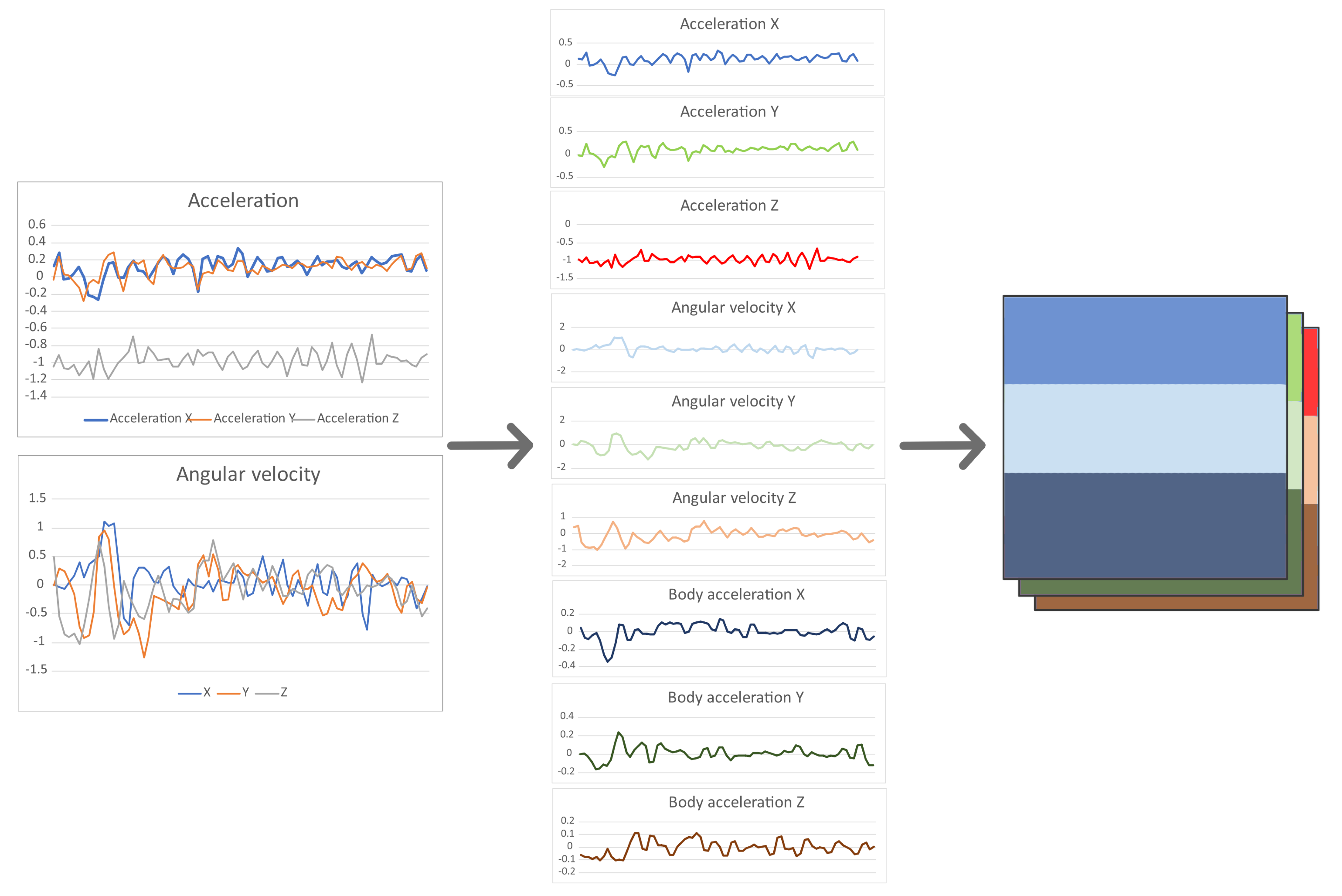
We start by analyzing the role played by different activities. For both neural network compression approaches—Any-Precision and SNN—we compute the per-activity average accuracy for all the compression levels and illustrate the results in
Figure 4. In the case of Any-Precision, we notice that some activities are almost always easy to classify correctly, regardless of the number of bits used in quantization, such as the case for lying down or going downstairs (here, only the 1-bit quantized model exhibits an accuracy drop). At the same time, the lowest accuracy is reported for sitting, where the top three quantized networks (4, 8 and 32-bit) all score similarly, at around 85%. Surprisingly, for walking downstairs and standing, the 2-bit quantized model yields the highest accuracy, which could be due to the regularization effect of quantization. In the case of SNN, we notice a more visible correlation between the compression level and the inference accuracy (as we slim the network, the accuracy drops); however, we again notice that some activities are more difficult to be accurately classified (e.g., standing) than others (e.g., laying), regardless of the network width. These results indicate that the appropriate compression level of the network should be chosen based on what we term
the difficulty of the input, which is influenced by the class to which the data point belongs.
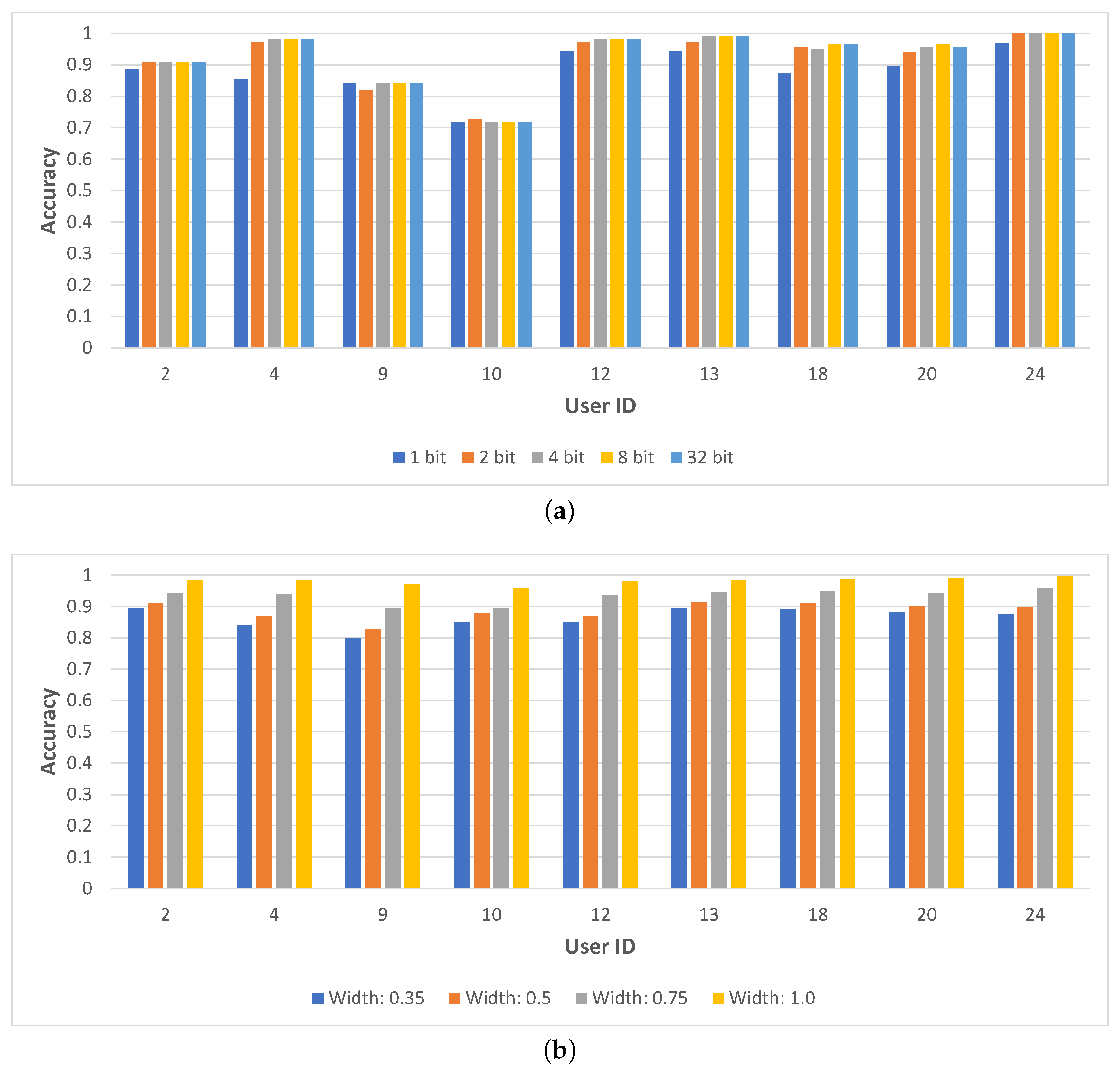
Next, we investigate the per-user differences in classification accuracy.
Figure 5 illustrates the accuracy per user (we select nine users randomly for illustrative purposes) and for each compression level for both networks. For Any-Precision, we notice important variations among users, with user 10 standing out due to a considerably lower accuracy for all networks (just above 70%) compared to the rest of the users (where on average the overall accuracy was higher than 90%). Interestingly, while the more compressed networks usually perform worse, the prominence of this effect is not the same across different users—for instance, the accuracy of inference for User 9 appears to exhibit no variation between 1-bit and 32-bit compression. In the case of SNN, we notice the same linear decrease in accuracy with the increase in slimming that is observable in the per-activity breakdown chart above. This relationship is present for all users, and the variations across users are smaller than in the case of Any-Precision.
The above analysis indicates that the classification success with different levels of compression varies from input to input and is influenced by contextual factors. These, according to our investigation, include the current physical activity and user-inherent factors; however, in different situations, other factors may play a role (e.g., device placement, etc.). Thus, our goal is to employ the maximum possible compression level that does not hurt the classification accuracy.
We first conduct a preliminary analysis on the feasibility of predicting the difficulty of the input, where a higher difficulty calls for a less compressed network. We aim to use a basic machine learning classifier in order to minimize the computational overhead of difficulty prediction.
Our difficulty predictors are trained as follows. First, we assign a label to each input sample, with a score between 0 and 1 representing the fraction of all the network’s compressed variants that achieved correct classification for that particular input. For example, if for Any-Precision and a given input datapoint, 3 out of the 5 levels of quantization correctly classified that input, the label would be
. For SNN, if 3 out of the 4 network widths had correct predictions, the label would be
. Next, we use the Orange data mining toolbox [
30] and train four basic machine learning models on the data: k-nearest neighbors (kNN), random forest (RF), support vector method (SVM) and linear regression. The goal was to correctly predict the difficulty score for the given input, and for comparison, we also included a dummy regressor which always predicted a constant value. Each input sample is comprised of all the 561 features pre-computed in the UCI HAR database [
28]. Finally, all 5 models were evaluated using five-fold cross-validation, and the mean squared error (MSE) and root mean squared error (RMSE) were used to assess the accuracy of the prediction. The results are provided in
Table 1 and show that the k-nearest neighbors algorithm delivers the best results in terms of correctly predicting the difficulty score for a given input sample.
While the above method enables input difficulty prediction, another proxy for this metric comes from the deep neural network itself. In a deep learning classifier, the final layer’s softmax function generates normalized classification scores, often termed confidence. The capability of the softmax confidence to accurately reflect the true confidence of the classifier was shown by Gu et al. [
31]. However, the authors note that calibration is needed in order to make it highly correlated with the expected accuracy. At the same time, however, Gal and Ghahramani argue that a model can be uncertain in its predictions even with a high softmax output, thus arguing against the term “confidence” [
32]. While we acknowledge that the interpretation of this term might be subject to debate, we pursue an analysis of how the softmax confidence scales with the accuracy that a neural network achieves for inputs of different activities when the network is compressed to a varying level.
Figure 6 plots the average confidence vs. average accuracy for the various compression levels for both Any-Precision and SNN on the UCI HAR dataset. This plot shows that there is a positive correlation overall between confidence and accuracy; that is, the network is more confident in the cases where it is also more accurate.
The relationship is not completely linear, and the accuracy cannot be robustly predicted from the softmax confidence. Nevertheless, there appears to be a certain connection between the softmax confidence and the accuracy. Besides, with the above standard machine learning methods, we examine the use of the network’s softmax confidence for guiding the network’s compression level.
4.2. Guiding Dynamic Network Compression with kNN
Returning to our goal of employing the maximum possible compression level that does not hurt the classification accuracy, we devise a method for automatically selecting the most appropriate DNN compression level for a given input.
We start from the observation that the kNN algorithm can forecast the difficulty of a given input for classification, and we evaluate the kNN’s utility for selecting the network’s compression level. For each sample from the training set, we compute the HAR prediction outcome (correct or incorrect) with each of the network compression levels employed. During testing, for each input, using the Euclidean distance between the features of the samples, the algorithm finds the k closest examples from the training set and selects the compression level which achieved the highest accuracy. In case of ties, the highest compression level is selected.
Three versions of the kNN algorithm are evaluated—for 20, 40 and 100 nearest neighbors—for both Any-Precision ResNet-50 and SNN MobileNet-V2. We choose these particular network models because they were previously successfully validated with the respective compression techniques [
11,
12] and were shown to achieve tolerable accuracy drop with increased compression (quantization/slimming).
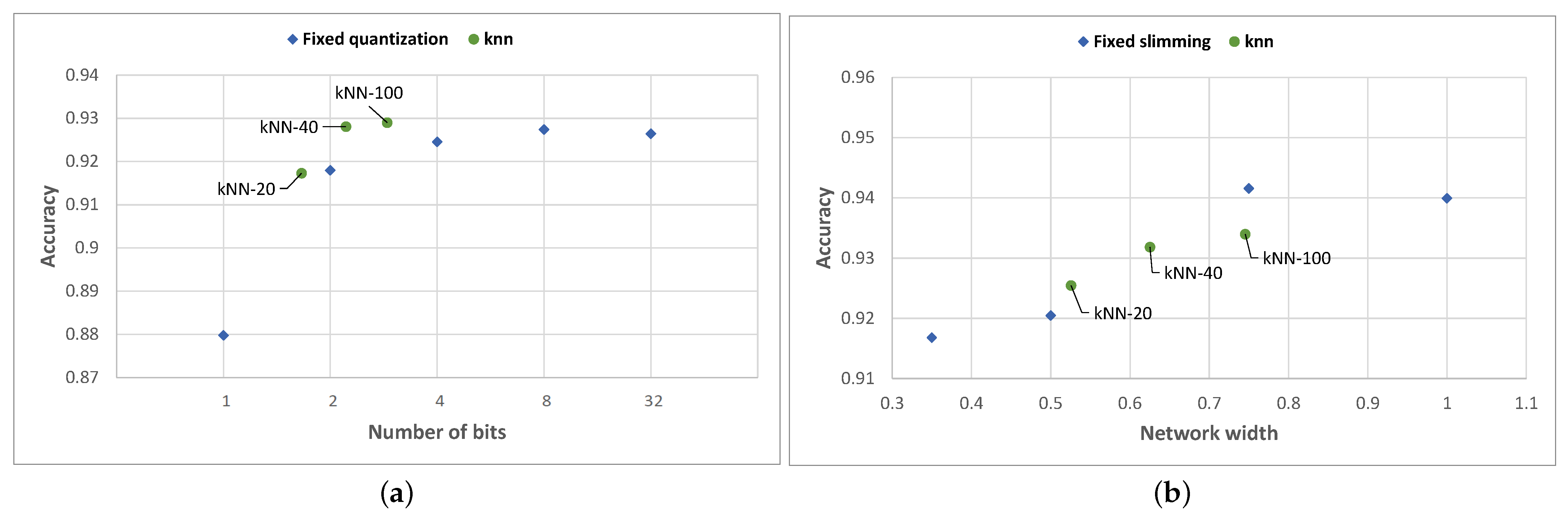
The results of the kNN algorithm are illustrated in
Figure 7 and show the average compression level selected by the kNN method, together with the HAR activity classification accuracy achieved.
In the case of Any-Precision ResNet-50, the results show that, for all flavors of the kNN algorithm, we improve the accuracy–compression trade-off; in addition, the green points remain above the Pareto front of the blue points. More specifically, kNN-driven adaptation achieves a higher classification accuracy compared to the accuracy achieved by the nearest static quantization level. Furthermore, the algorithm using k = 100 scores even higher in terms of accuracy compared to any static quantization level. This paradox is explainable by those situations in which a more quantized network (that may be selected by the kNN algorithm) for a given input is more accurate than a non-quantized network.
In the case of SNN MobileNet-V2, we notice a lower performance of the k-NN compression selection algorithm. The algorithm slightly outperformed static slimming for values of k equal to 20 and 40, but for k = 100, it failed to reach the accuracy achieved by the 0.75-width network.
4.3. Guiding Dynamic Network Compression with Softmax Confidence
The above kNN-based approach may lead to very good results (i.e., simultaneous energy savings and accuracy increase in case of Any-precision), but it does not allow the fine-tuning of the operational point—it always aims for the highest possible accuracy. Often, however, the accuracy may be traded for increased energy efficiency. Thus, we now develop another approach that in a hierarchical manner first determines to which difficulty group an input point belongs and then allows the selection of an appropriate neural network compression level yielding the desired accuracy/energy trade-off.
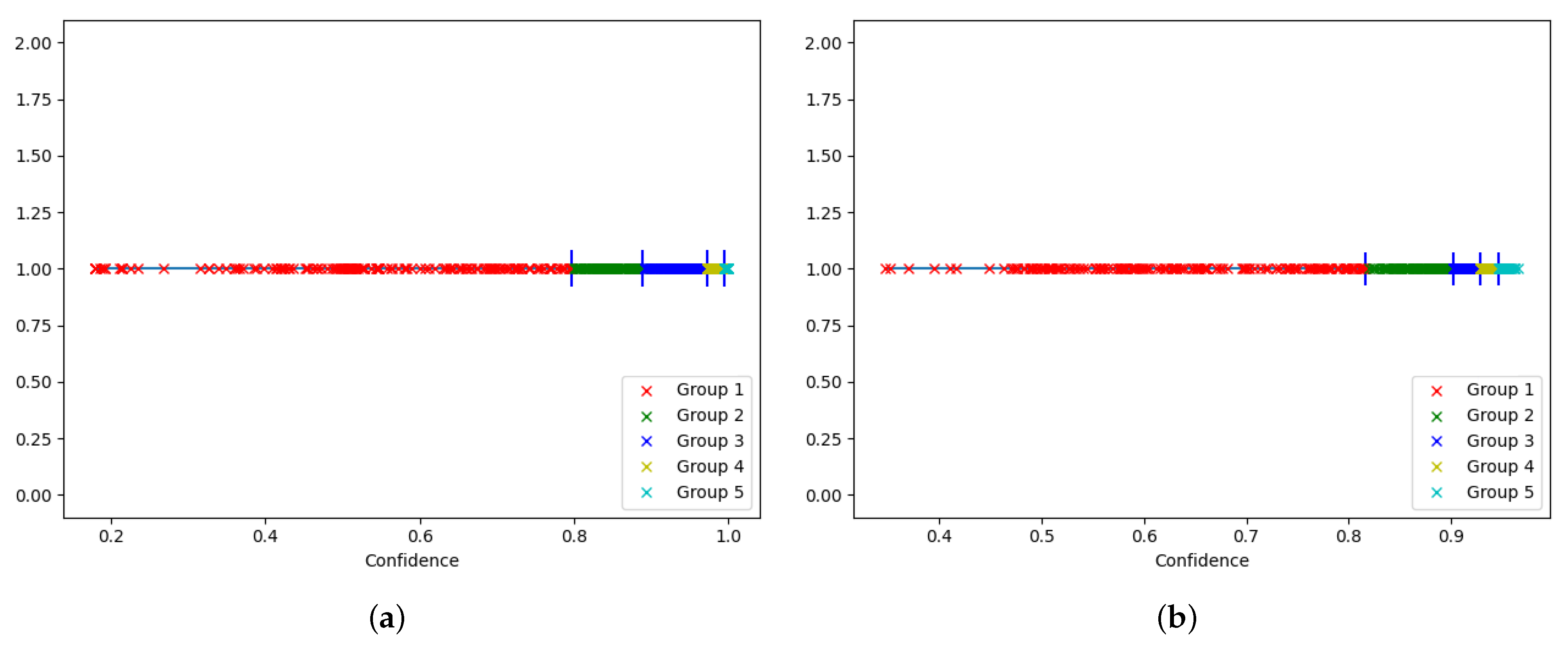
We now use the softmax confidence to guide the compression level selection algorithm. Based on the near-linear relationship between the accuracy and the confidence, we group inputs with similar prediction confidence together, as this indicates that these inputs are of a similar difficulty, thus tolerating the same level of neural network compression in order to be classified accurately. We empirically establish the number of groups and confidence interval for each group based on the prediction confidence obtained using the most compressed network (i.e., 1-bit Any-precision or 0.35%-width SNN) on the training set. We choose the group boundaries in order to obtain a balanced distribution of the samples in each group. The grouping based on the softmax confidence of the training set input samples for both networks is illustrated in
Figure 8.
After assigning each training input to a group, we then compute the average accuracy obtained by each network compression level for each of the groups. For each group, we then construct a linear model defining the relationship between the compression levels (which are encoded as numerical values; i.e., 1b–1, 2b–2, 4b–3, 8b–4, 32b–5 for Any-Precision, and 35%–1, 50%–2, 75%–3 and 100%–4 for SNN) and the corresponding accuracy achieved at a certain compression level. To build the model, we use the average accuracy values recorded on the training set when different network compression levels are employed. We then use this model to predict the most appropriate compression level for a given target accuracy.
The above set of linear relationships between the expected classification accuracy and the employed compression level that we have constructed for each of the input difficulty groups allows us to quickly identify the most appropriate compression level, should we have the softmax confidence information to hand. Thus, in the initial softmax-based approach, we first classify an incoming sample using the most compressed network model and then, based on the confidence of that prediction, we assign the input to one of the difficulty groups. If the corresponding linear model indicates that the most compressed model is the most appropriate (for the desired target accuracy), we keep the calculated classification result. Otherwise, we repeat the classification using the compression level indicated by the linear model.
The downside of this approach is that for some input samples the classification will be performed twice—in case the linear model indicates that the most compressed network is the best choice. Repeated classification may induce an overhead, diminishing the energy savings achieved through NN compression. Therefore, we devise an alternative approach where the compression level selection is guided by the confidence of the previous datapoint prediction. We base this approach on the fact that natural human mobility is not characterized by rapid variations; thus, rapid variance among subsequent data points is unlikely [
33,
34]. To further validate this hypothesis, we compute the correlations between each pair of consecutive prediction confidence values when running the network on consecutive training samples from the dataset, and we obtain a value of
indicating a medium-strong correlation [
35].
We evaluate both approaches on the UCI HAR dataset for both Any-Precision and SNN. The target accuracy threshold can be adjusted according to the requirements for achieving either a higher accuracy or a higher energy efficiency. In our evaluationl we varied the target accuracy from 0.8 to 0.99 to illustrate how the accuracy–energy savings trade-off translates into actual benefits brought by the dynamic adaptation framework.
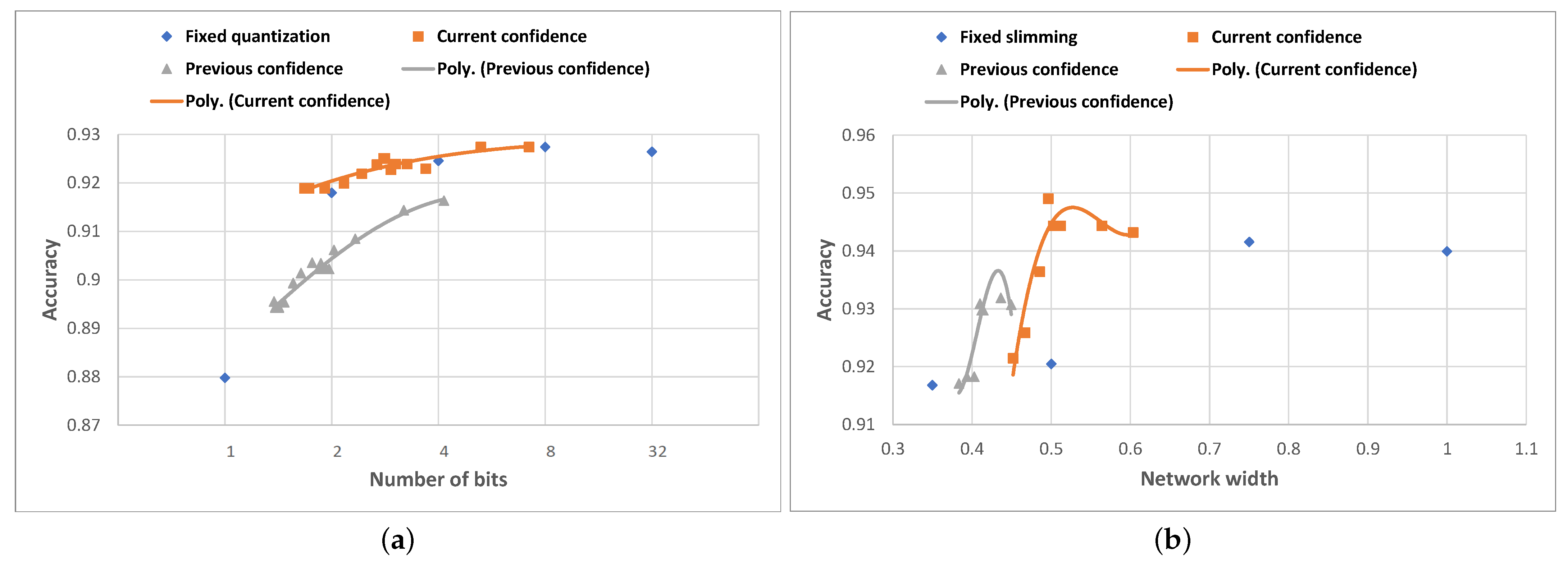
The evaluation results are displayed in
Figure 9. In the case of Any-Precision Resnet-50, we notice that the first approach (using the current confidence) achieves average accuracy scores slightly higher than those obtained using fixed quantization, but using more compressed networks on average, and thus saving more resources. Using this approach, a maximum average accuracy of
can be achieved with an average quantization level of
bits, which is equal to the maximum average accuracy obtainable using fixed 8-bit quantization. The results of the second approach (using the prediction confidence of the previous sample) are worse, however—the average accuracy is 1–2% lower than that obtained using fixed quantization, for the same quantization level. A possible explanation for this could relate to a poor correlation between the confidence of consecutive samples, very likely caused by the fact that grouping intervals are determined using the confidence scores from the most compressed network, while the algorithm selects the group based always on the previous confidence, which is computed using various network compression levels.
In the case of the SNN MobileNet-V2, both approaches yield better accuracy results compared to setting the same compression level for a static network. The first approach outperforms even the case of always running the 100% width network, with an average width of the compression levels of 50%. The second approach again underperforms for the same reasons as stated above, but in this case, it still scores better in terms of accuracy than choosing the equivalent static network compression level.
4.4. Guiding Dynamic Network Compression with LDA
So far, we have developed network compression adaptation methods based on the similarity among input datapoints’ features; i.e., the kNN approach and based on the grouping of inputs according to the softmax confidence scores. None of the methods is without its weaknesses. The kNN approach requires that the whole training set containing 561-dimensional data points should be stored on the device, which may be prohibitively expensive for resource-restricted mobile devices. The confidence-based approach, on the other hand, may require repeated classifications of the same input, essentially wasting energy.
We therefore develop an alternative approach for grouping inputs in difficulty levels by using a well established statistical method—linear discriminant analysis (LDA). LDA finds a linear combination of features that best separates classes observed in the training set. We develop two flavors of the LDA-based dynamic network compression adaptation algorithm. In both cases, we apply LDA on the space of input samples from the UCI HAR training set. Given that the input samples have a considerable number of features (561) which may result in the overfitting of the LDA algorithm, we reduce the dimensionality of the inputs using the principal component analysis (PCA) to 10 values per input sample before applying LDA.
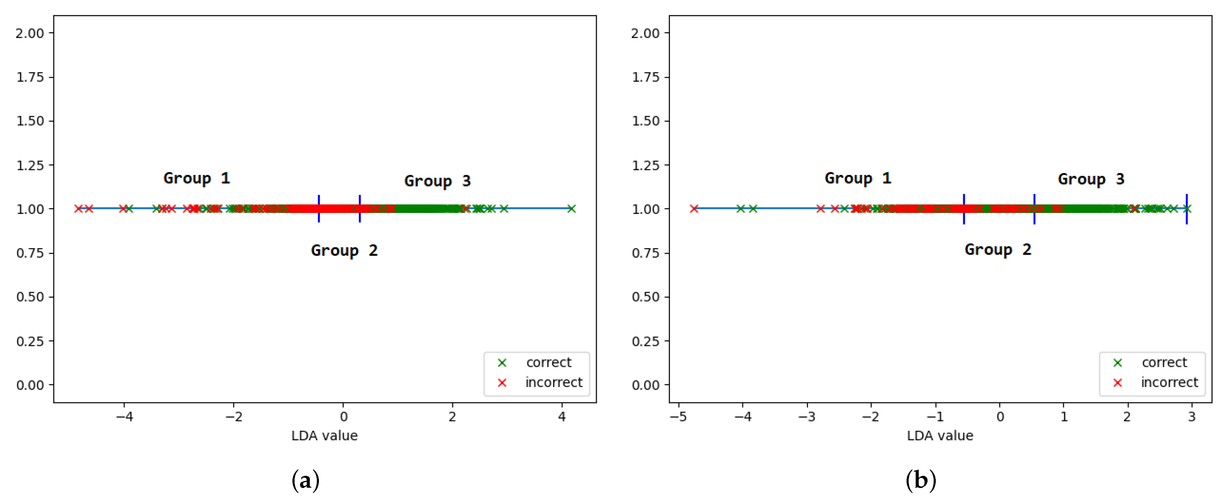
The first flavor of our algorithm uses LDA to find the subspace that best separates the inputs based on the difficulty of classifying them. To obtain a label that guides the LDA grouping, we classify each sample with all compression levels of the network. For each input, we get a set of predictions, some of which may be correct and some incorrect. We then assign each sample a score between 0 and 1 based on the number of compression levels that correctly classified that sample. We then determine the groups by combining the elements according to their position in the resulting subspace, so that inputs with a similar “difficulty” level (how likely they are to be classified correctly) are aggregated together in the same group. An illustrative example for this “correctness”-based grouping is presented in
Figure 10.
In the second flavor of the algorithm, we start from the previous observation that the actual physical activity influences the difficulty of the input and ultimately the accuracy of the network. As such, we apply LDA to separate the input vectors according to their activity class label, where we combine walking, walking upstairs and walking downstairs into dynamic and sitting, standing and lying down into static classes. The same principle for LDA grouping as with the first algorithm flavor is then applied, resulting in the “movement”-based grouping.
After establishing the groups, in both versions of the algorithm, the approach for constructing and assigning a linear accuracy-compression level model to each group (described in
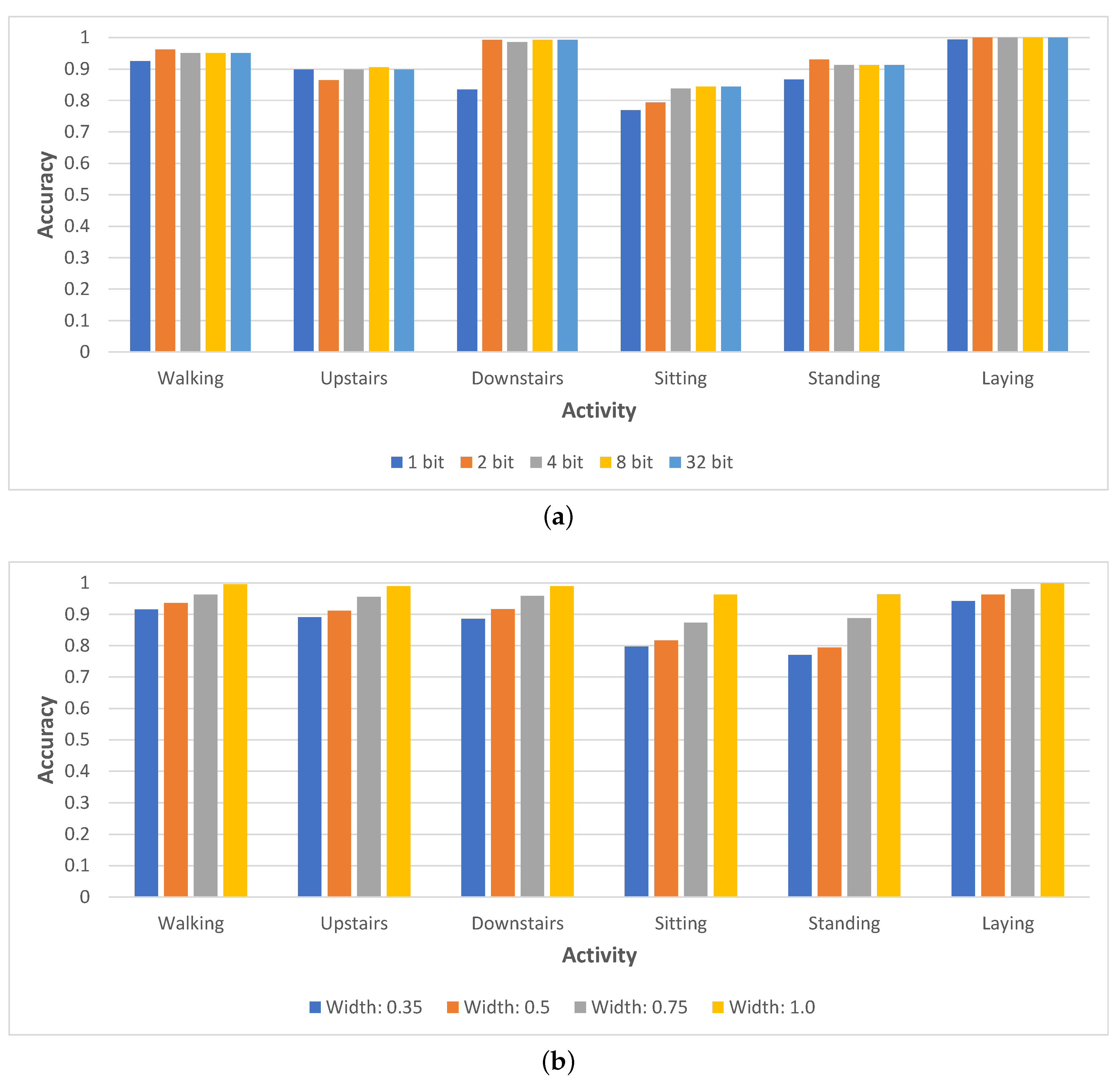
Section 4.3) is used. We evaluated both algorithms on both networks for the UCI HAR dataset, and the results are illustrated in
Figure 11.
For Any-Precision ResNet-50, the “movement”-based version of the algorithm scores very similarly in terms of average accuracy and average quantization level to the fixed quantization approach for 1, 2 and 4-bit quantization. However, it does not reach the highest average accuracy achievable with the fixed 8-bit quantization. The “correctness”-based algorithm generally scores slightly lower in terms of average accuracy compared to the “movement”-based counterpart for the same average quantization levels.
In the case of SNN MobileNet-V2, however, the results show that both versions of the algorithm are able to clearly outperform the results obtained using fixed slimming in terms of average accuracy, for all fixed slimming ratios, thus being significantly more resource-efficient. The highest average accuracy of is achieved by the “correctness”-based algorithm with an average network width of , which is higher than the maximum average accuracy achieved using fixed slimming ( obtained using the width network). The “movement”-based algorithm scores slightly lower in terms of average accuracy than its “correctness”-based counterpart, but still outperforms fixed slimming across all network widths.
4.5. Comparative Analysis
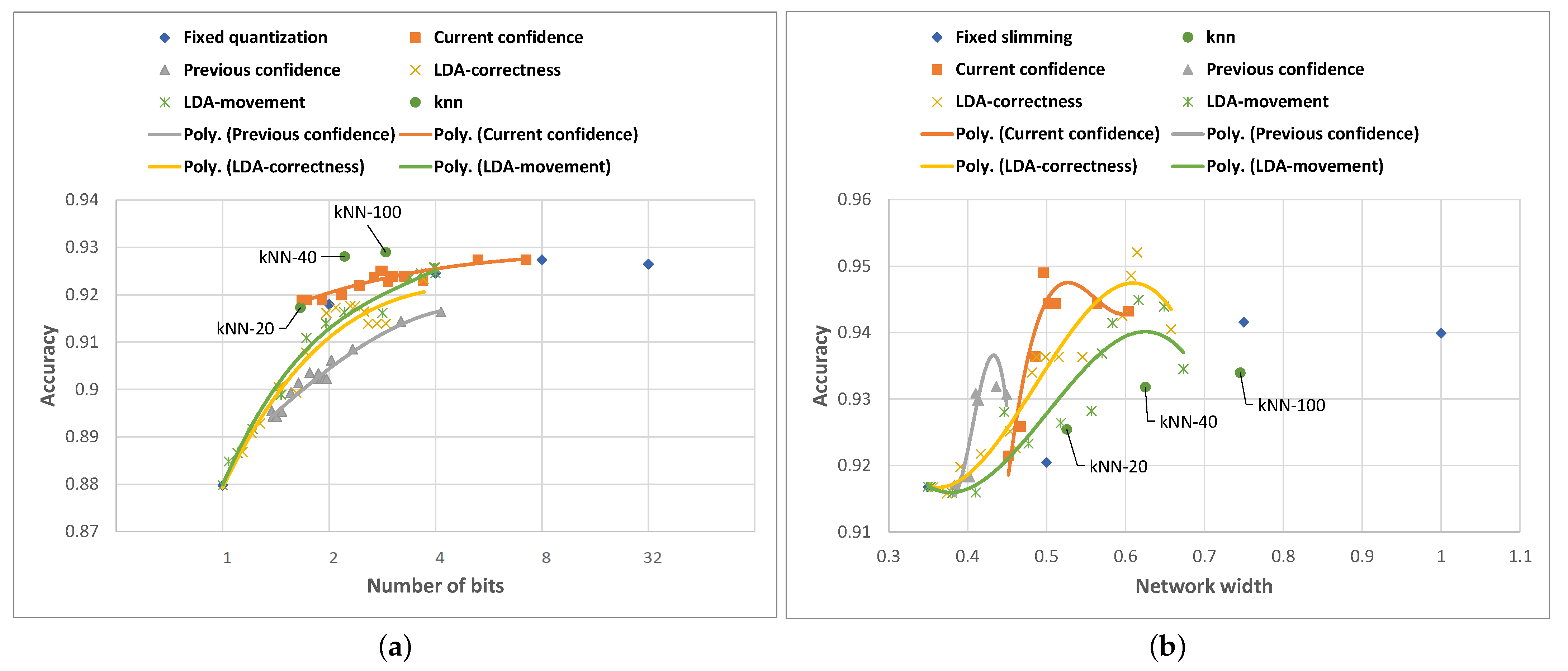
Following the evaluation of all the proposed algorithms for both Any-Precision and SNN networks, we provide a comparative analysis of the results in
Figure 12. We note that the kNN-based adaptation always aims for the best possible accuracy with the smallest amount of resources used, while the confidence-based and LDA-based adaptation allows the fine-tuning of the trade-off between the compression and the inference accuracy. Thus, for the kNN, we observe only individual points in the compression (e.g., number of bit or network width) vs. accuracy space, whereas the other approaches draw a trade-off line in this space.
We observe that the algorithms perform differently on the two networks: for Any-Precision ResNet-50, compression level adaptation based on kNN-100 delivers an improvement in both the accuracy and the resource usage over any single static compression choice. The remaining algorithms indeed allow the fine-tuning of the accuracy–resource usage trade-off, but they do not appear to deliver the improvements brought by the kNN approach. This is not to say that such approaches do not have their place—indeed, they allow us to achieve intermediate accuracies not supported by the discrete compression levels implemented for a particular neural network.
For SNN MobileNet-V2, the kNN-based approach does not improve the classification accuracy beyond that delivered via static compression. On the other hand, the methods harnessing LDA and confidence-based adaptation not only enable the fine-tuning of the accuracy–compression trade-off but also result in accuracies higher than those delivered by the static compression (or even an uncompressed network).
When analyzing these results, it is important to take into account the overhead induced by individual algorithms in terms of resource/energy consumption. The softmax confidence-based algorithm involves running the inference on the same input twice for some cases, while the k-NN has the disadvantage of high memory requirements due to the need to store all the training data on the device. As such, choosing the best compression level selection algorithm is not a trivial task and requires taking into account the resources available on the device, the specifics of the application and the context of use. Due to its low storage requirements and the ability to adapt the compression level without the need for multiple classifications of the same data point, in the rest of the paper, we focus on the LDA-based algorithm and proceed with its practical implementation.
5. Dynamic DNN Compression on Mobile Devices
After successfully validating various methods for dynamic DNN compression adaptation on the publicly available UCI HAR dataset [
28], we proceed to demonstrate its applicability in a real-world experiment. We focus on the MobileNet-V2 Slimmable Neural Network. Network slimming directly maps to a reduced number of operations and thus is bound to bring certain energy savings. The Any-Precision approach, as discussed in
Section 3.1, relies on quantization, which need not translate to actual energy savings on 32-bit or 64-bit hardware. We also focus on a single dynamic compression adaptation algorithm—correctness-guided LDA—as it provides the balance between the computational overhead and the classification accuracy on the SNN MobileNet-V2 HAR network (see
Section 4.5).
5.1. Implementation
We implement our approach on the UDOO Neo Full board, a compact IoT embedded computing device equipped with a three-axis accelerometer and a digital gyroscope. We chose this platform as its processing hardware corresponds to that found in today’s low-end smartphones; however, the platform itself runs Linux enabling a quick prototyping of dynamic DNN adaptation (at the time of our experiments, Android’s TensorFlow Lite framework did not allow dynamic neural network graph reconfiguration). We sample the acceleration and angular velocity in all three axes from the board’s sensors with a frequency of 50 Hz using the Neo.GPIO library [
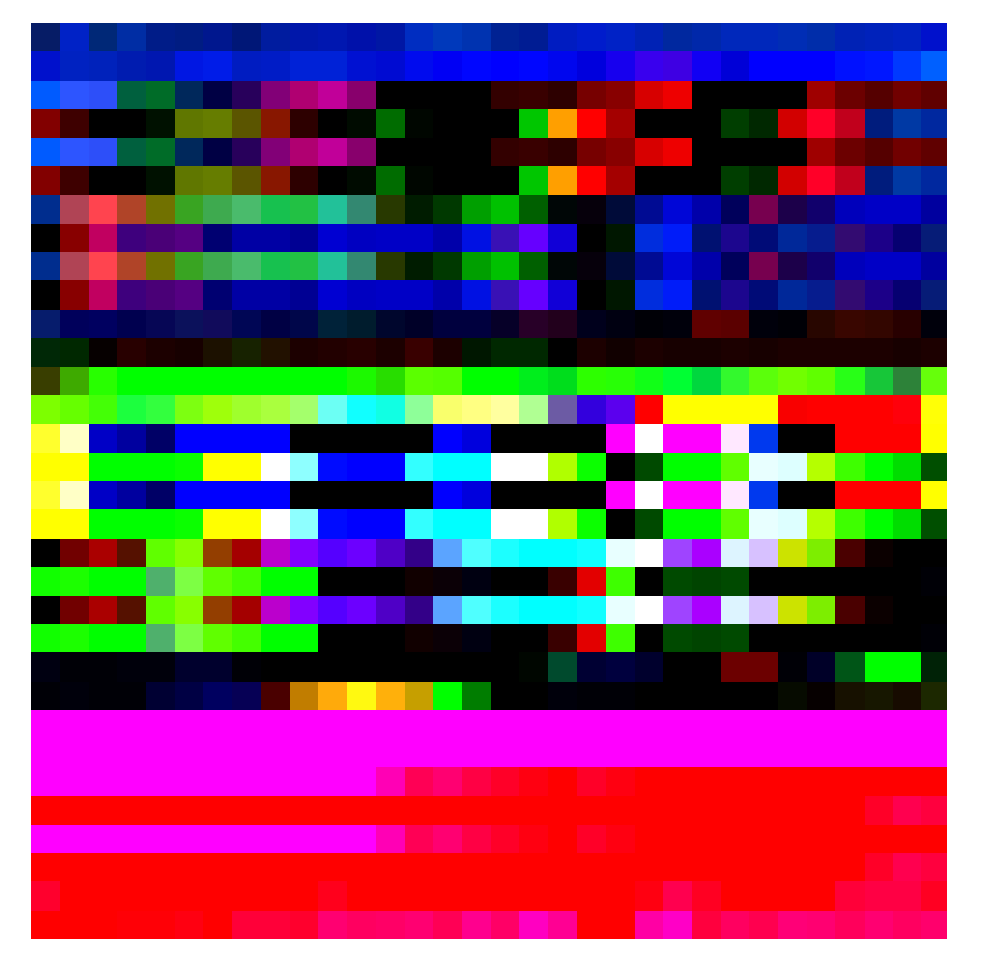
36]. The raw readings were saved to a local file (for subsequent additional analysis) but also went through a processing pipeline similar to the one used in the UCI HAR dataset. This consisted of noise removal followed by the separation of the acceleration into high and low-frequency components, resulting in nine numeric values for each sample: the three total acceleration values (high-frequency components), three angular velocities and three body acceleration values (low-frequency components). The samples were grouped into windows of 128 measurements with an overlap of 64 measurements to match the pre-processing of the original dataset. The measurements were then combined to form 3D images in the same way as described in
Section 3, which were then taken as inputs by the SNN.
In addition, from the filtered signals, we also calculated the values of 55 features (see
Table 2) that we used as an input for the compression level selection algorithm. This represents a sub-set of the total of 561 features used when evaluating the compression rate selection algorithms in
Section 4; we chose only a subset in order to reduce the computational burden given the resource constraints of the UDOO board. The chosen compression rate selection algorithm was the LDA based on “correctness” grouping, which was shown to yield the best trade-off between the accuracy of the classification and resource/energy efficiency following the comparative evaluation of the algorithms performed on the UCI HAR dataset (as shown in
Section 4.5). In the experiments, the target accuracy level for the algorithm was set to
. To select the most relevant features, we used the RReliefF algorithm [
37] and evaluated all the features based on how accurately they describe the correctness of the classification. This analysis revealed that the time-domain features yield significantly better results than the frequency-domain features. Hence, we disregarded the computation of the latter and considerably improved the overall computation speed of the feature extraction process.
Consequently, for each input, our algorithm computes the 55 features, applies the compression rate selection algorithm and selects the width of the SNN which then performs activity inference. The entire framework’s workflow—i.e., acquisition, pre-processing, compression level selection and activity inference—was performed on the UDOO Neo Full board in real time. The software saved the inference results in a local log file but also printed them to a terminal for real-time inspection via a wireless connection.
5.2. User Study Details
We evaluate the performance of our approach in terms of inference accuracy vs. energy savings enabled by the dynamic DNN compression selection algorithm on the human activity detection task. Our study involved 21 volunteers: 13 male and 8 female participants, with an average age of 29 and a standard deviation of 12 years. Our adaptation approaches were initially developed and evaluated on the UCI HAR dataset (see
Section 4; thus, we ensure that our study is conducted under similar conditions to those described in the original study. Namely, the participants were equipped with a battery-powered UDOO board placed to replicate, as accurately as possible, the positioning of the smartphone in the original UCI HAR experiment, and the activities conducted in our guided scenario are the same as those used in the original UCI HAR experiment.
The experiments were conducted in a university campus building at our institution’s premises. The volunteers performed all six activities in a row. They first sat in a chair for two minutes without leaning against a table. They then stood still for two minutes, followed by two more minutes of lying down. After completion of these three static activities, the volunteers walked up and down a hallway, which lasted from two to three minutes. This was followed by walking down and up the stairs. In doing so, we were limited by the total number of stairs, so the walk in each direction took about 45 s.
5.3. Experimental Results
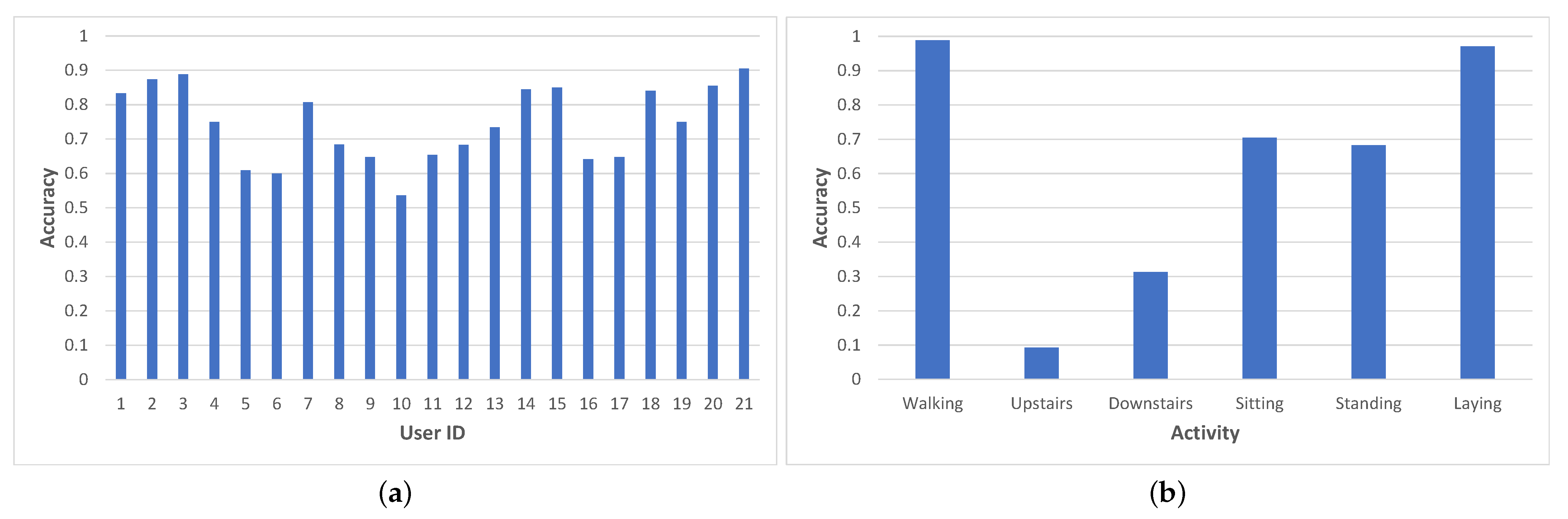
Our dynamic mobile deep learning adaptation network achieved an overall average accuracy of 74.6% for all users in this study. This accuracy is lower than that achieved by the framework on the UCI HAR dataset, which is to be expected given that the network was trained on that dataset and now used to infer the activity based on samples collected in a different environment, on a different target group of users and with different hardware. Factors such as the different positioning of the device on the body of the user, different geometry of the chair and stairs compared to those used for creating the dataset may all impact the outcome of the classification, which overall still achieved relatively high accuracy.
In particular, our study showed the framework to exhibit high variations between users, as shown in
Figure 13a. For nine users, the average accuracy was over 80% (with a max accuracy of 91%), while for five users, the values were below 70%, with the lowest being 54%.
We analyze the accuracy variation among the different activity states and illustrate it in
Figure 13b. This analysis also reveals important variations: activities such as lying or walking can be inferred with a high accuracy (almost 100%), while other activities are more difficult to classify correctly. Sitting and standing are often confused by the network with one another and thus exhibit a slightly lower accuracy (around 70%); this can be explained by the similarities in terms of acceleration and angular velocities for these two activities. The worst classification accuracy is reported for walking upstairs and downstairs (under 40%), with one possible reason being the geometry of the staircase used for performing the experiments (a half landing staircase—U shaped—which implies that the user performs a 180° turn every half floor).
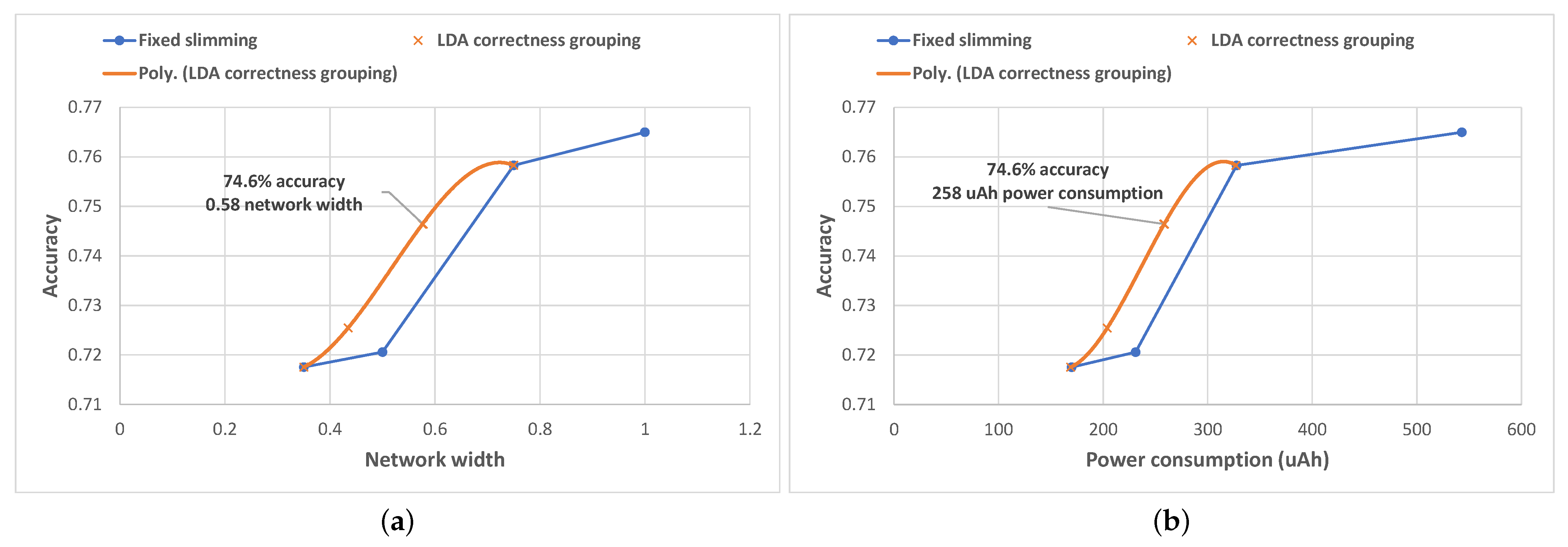
We then further explored the analysis of the efficiency of our LDA-based compression level selection algorithm during this user study and investigated the relationship between the average classification accuracy and the average network width and average power consumption, respectively. During the experiments, the sequence of network width selections performed by the algorithm resulted in an average accuracy of
and an overall average width of the SNN of
(see
Figure 14a). In terms of accuracy, this scores higher than the accuracy obtained by using a fixed width of either 35% (
) or using
of the network (
) and slightly lower than using either the
or the
fixed width networks (which achieved an accuracy of
, and
, respectively).
In addition, we performed the post processing of the results in order to illustrate the performance of our algorithm for the entire range of possible target accuracy values in more depth. We plot all resulting datapoints together with their corresponding trend-line in
Figure 14a and notice that our algorithm outperforms the results obtained by using fixed slimming, achieving a higher accuracy (the trend-line is always above the fixed slimming line) for the same network width, and thus is more resource-efficient.
5.4. Power Consumption Evaluation
In order to assess the power consumption of our LDA-based compression level selection algorithm on the MobileNet-V2 SNN, we measure the power consumption of running inference using each SNN width, together with the additional power consumption required by the adaptation algorithm. We perform the measurements on the same device used during the real-world experiments, the UDOO Neo board, using the Monsoon power monitor tool [
38]—a high sampling frequency platform commonly used for power measurements in mobile and embedded computing [
39]. The power consumption for performing inference using each of the fixed slimming widths of the MobileNet-V2 SNN is depicted in
Figure 14b.
To assess the overhead induced by the LDA-based compression level selection algorithm, we performed power measurements on the UDOO board during inference with the MobileNet-v2 SNN with and without the algorithm and compared the results. Using the algorithm induced no measurable overhead in terms of power consumption, with the resulting power consumption readings for the two cases being almost identical (4.88 mAh vs. 4.87 mAh for running classification on all the UCI HAR test-set samples with and without the compression level selection algorithm, respectively).
Based on these measurements, we were able to assess the energy savings brought by our algorithm during the real-world study. These results, illustrated in
Figure 14b, show that compared to to the top two network widths, the adaptation algorithm achieved considerable energy savings: an average power consumption of
compared to
for the fixed
width network and
for the fixed
network). Analyzing the power consumption across the entire range of possible target accuracy values, we again notice that our algorithm outperforms fixed slimming in terms of energy efficiency: to achieve the same average accuracy, the algorithm consumes less power.
6. Discussion
Our framework enabling self-adaptive mobile deep learning solutions can easily be integrated with any neural network compression method that enables real-time adjustment of the compression level. As such, it has the potential to foster the deployment of neural networks on resource-constrained devices where the operation is hindered by the networks’ inherent complexity. By enabling neural networks to operate, albeit approximately, under even scarcer resources, a wide range of embedded devices can develop to become edge computing platforms: from wearables, smart speakers and smart appliances, to earables and smart toothbrushes. Consequently, our approach represents an important contribution to the Artificial Intelligence of Things (AIoT) [
40], the newly emerging research area resulting from the synergy between AI and IoT. In this context, our solution enables DL models to self-adapt in real time to the dynamic and varied IoT application scenarios, contexts of use and platform resources (i.e., computation, storage and battery resources) available in each particular use case.
In the experiments described in this paper, the selection of the appropriate network compression level at each inference step was driven by the estimated “difficulty” of the input; however, our algorithms also allow for an environmental adaptation of the network’s compression, driven for example in an IoT use case by the constantly changing environmental context including application data, knowledge base, task-related performance requirements and platform-imposed resource constraints. This enables an on-demand model compression which can achieve the desired balance between the model’s performance and the environment’s budget, reducing costs and improving computational efficiency with negligible performance degradation.
In addition, our approach’s applicability is not limited to resource-constrained embedded computing nodes in the IoT but can be applied in any “sensing” scenario where computing resources or the available energy budget are limited. One such example is Unmanned Aerial Vehicle (UAV)-based Earth Observation imagery applications, where the on-board resource usage directly impacts the flight autonomy of the device. In such cases, our algorithms can self-adapt the network compression to optimize the resource usage based on the
difficulty of the image for the given task (e.g., in weed detection applications, the crop particularities such as type or growth stage significantly impact the difficulty of the processing task [
41], opening the door to important energy savings if
easier images are processed using the
more compressed networks).
While we demonstrated our framework on both Any-Precision and Slimmable Neural Networks, only the latter showed its practical viability for achieving important energy savings. For the latter, the compiler-level support for enabling the quantization of the network’s parameters to be translated into an actual reduction in the number of bits used for computations at the CPU level is still missing. As of the time of writing this manuscript, the native support for dynamic quantization during inference provided by PyTorch remains limited to 8 bits on CPUs (GPU support is not available). Future research directions could address these limitations through custom implementations using custom machine learning compiler frameworks, such as TVM [
27].
7. Conclusions
In this paper, we introduced a framework for dynamic mobile deep learning adaptation which aims to translate the theoretical advantages advertised by the recent neural network compression techniques into real-world resource and energy savings on ubiquitous computing devices.
We exemplify the operation of the framework using two of the most promising neural network compression techniques—Any-Precision [
12] and Slimmable Neural Networks [
11]—both of which allow the dynamic selection of the compression rate during inference (either the number of bits used for quantization or the width of the network, respectively). As a use case, we choose human activity recognition on a smartphone, and we train both networks on the publicly available UCI HAR dataset [
28].
Starting from the analysis on context-related factors impacting the accuracy of the classification and the difficulty of the input, we introduced three algorithms for the dynamic selection of the compression rate during inference (kNN, softmax confidence and LDA subspace projections) and assessed their performance for both neural network compression techniques on the UCI HAR dataset. The three-way comparison of these algorithms confirmed their feasibility in offering a scalable trade-off between the inference accuracy and the resource usage and revealed that selecting the most appropriate algorithm depends on the neural network model and compression technique used, but also on the constraints in terms of hardware resources and context of use.
The user study we conducted to confirm these theoretical findings validated the proposed framework both in terms of the accuracy of the classification and in terms of the efficiency of the compression level selection algorithm compared to using a static neural network compression level. In the study, we configured our framework with the LDA correctness-based grouping algorithm on the SNN MobileNet-V2 network and achieved an accuracy of while using only of the network width. Compared to applying a fixed network width of , our framework used less energy with only a drop in the average accuracy of the classification.
The results obtained and presented in this paper confirm that our self-adaptive approximate mobile deep learning approach has the potential to foster the deployment of deep learning on resource-constrained computing devices by enabling neural networks to scale their resource usage and thus their energy consumption, according to environmental factors and context of use, with negligible accuracy drops.


