
Predicting Out-of-Stock Using Machine Learning: An Application in a Retail Packaged Foods Manufacturing Company


Abstract
:1. Introduction
2. Literature Review
2.1. The out of Stock Problem: Drivers and Consumer Response
2.2. Out of Stock: Detection and Prediction
3. Methodology
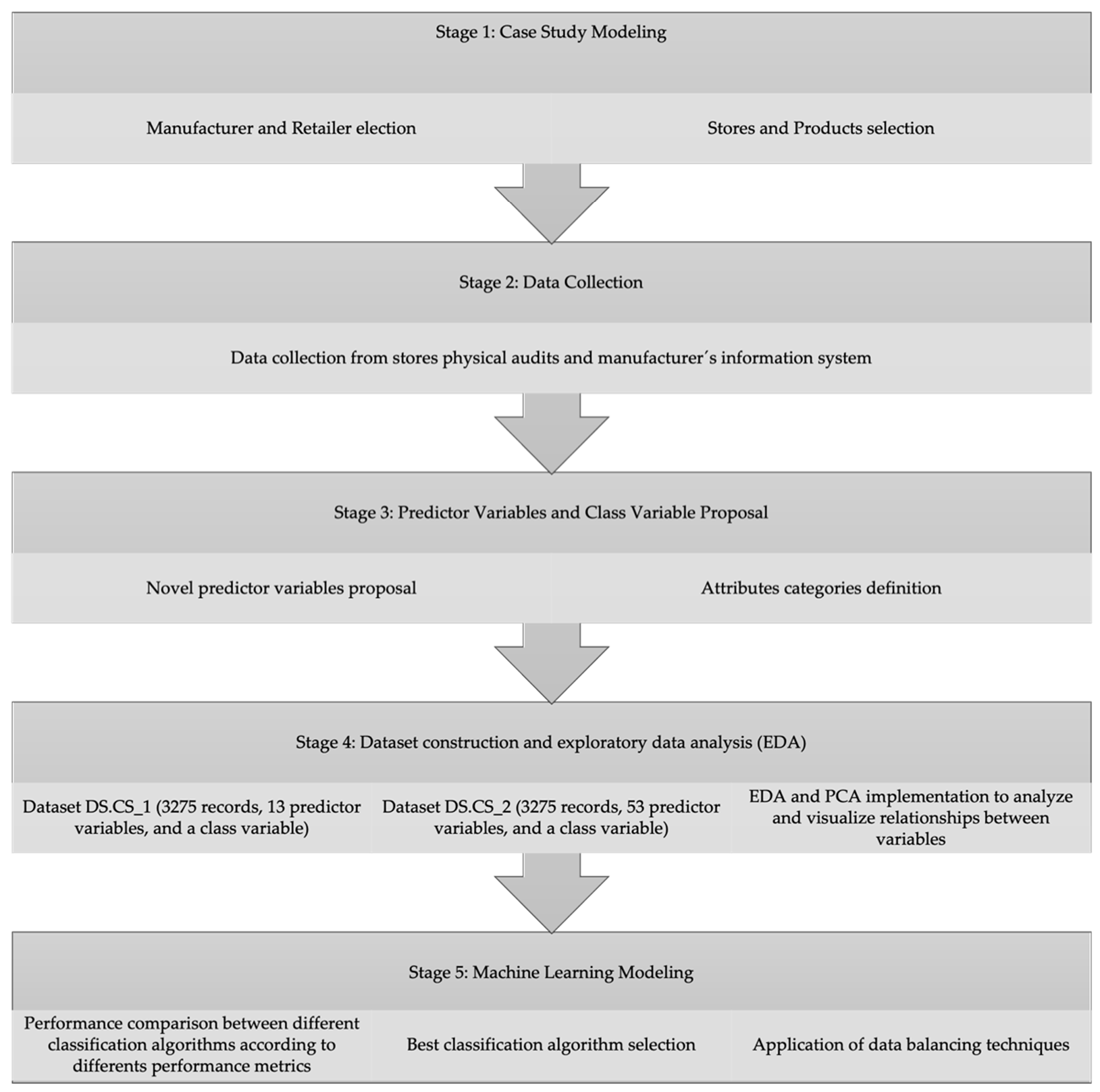
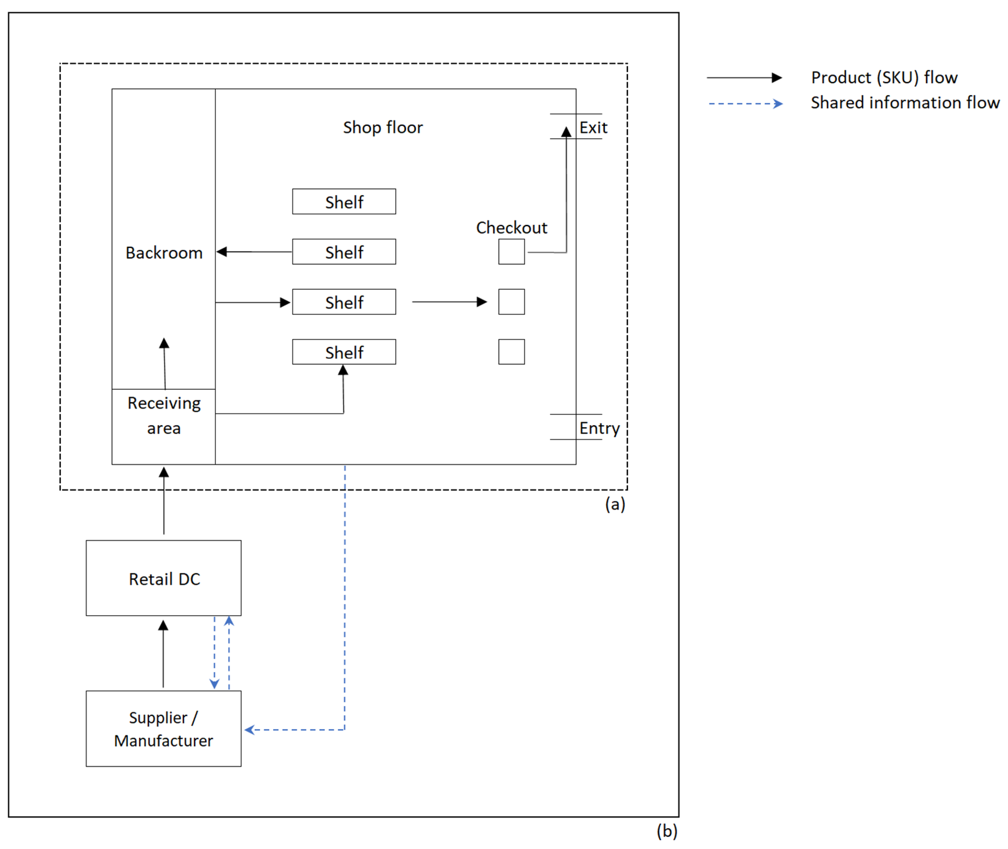
3.1. Case Study Modeling
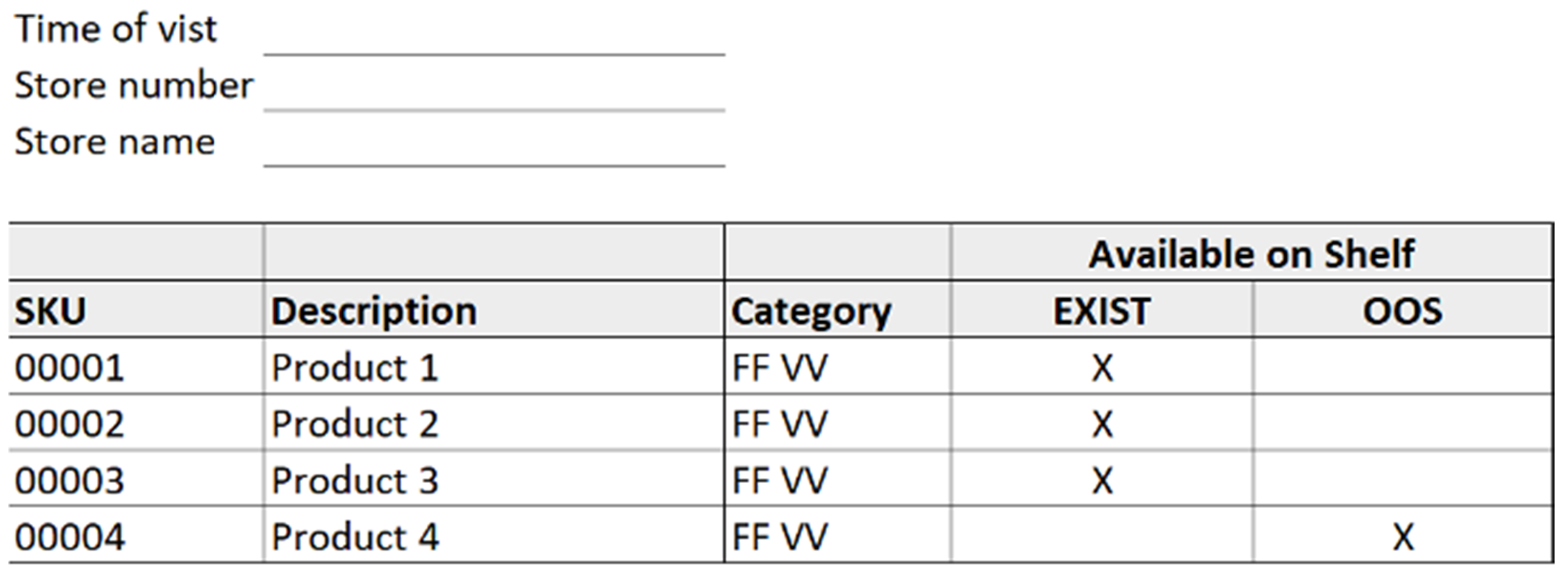
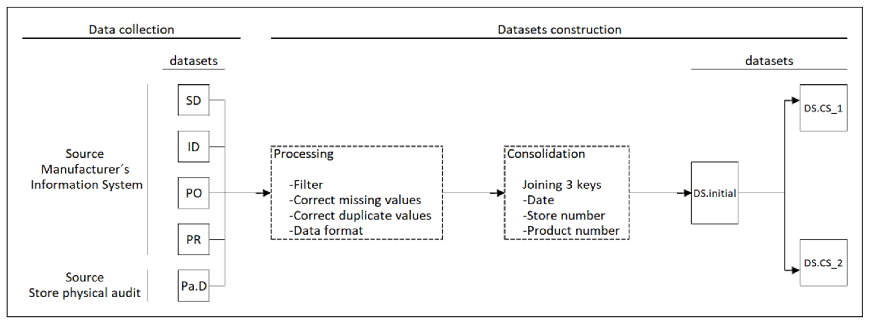
3.2. Data Collection
3.3. Predictor Variables and Class Variable Proposal
- Sales features describe the sales of each pair product-store for a time period.
- Inventory features present information on inventory records, In stock, and adjustments for each pair product-store for a time period.
- Product features describe the product’s inherent characteristics.
- Context features present information regarding external variables that impact certain aspects of the product.
- Ordering features contain information regarding the purchase orders issued to the manufacturer and received by the retailer for each product-store for a time period.
- Supply chain features describe logistics and replenishments methods.
- Description features present categorical data for the identification of products, stores, and purchase orders. It also includes date data.
3.4. Dataset Construction and EDA
- DS.CS_1 contains only some of the predictor variables presented in [7]. The predictor variables selected were 13 and correspond to the main ones in terms of information gain. The DS.CS_1 dimension was 3275 records, 13 predictor variables, and a class variable.
- DS.CS_2 was built with 13 predictor variables selected from [7] and 40 new predictor variables proposed in this work. The DS.CS_2 contained 3275 records, 53 predictor variables, and a class variable. The unimportant variables, such as description features, were not considered in these three datasets.
3.5. Machine Learning Modeling
- RF hyperparameters for DS.CS_1 was number of trees = 900 and number of variables to possibly split at in each node = 6. The hyperparameters for DS.CS_2 was number of trees = 600 and number of variables to possibly split at in each node = 6. The range of values studied for number of trees was 1 to 1000, and for the number of variables to test for a possible split in each node was 2 to 7.
- DT hyperparameter for DS.CS_1 was the maximum depth of any node of the final tree = 3. The hyperparameter for DS.CS_2 was the maximum depth of any node of the final tree = 4. The range of values studied for the maximum depth of any node of the final tree was 1 to 30.
- rSVM hyperparameter for DS.CS_1 was cost of constraints violation = 1 and sigma = 0.4. The hyperparameter for DS.CS_2 was cost of constraints violation = 1 and sigma = 0.3. The range of values studied for cost of constraints violation was 1 to 10, and for sigma was 0 to 1, in sequences of 0.1.
- NNET hyperparameter for DS.CS_1 was size = 20 (number of hidden units) and decay = 0.50. The hyperparameter for DS.CS_2 was size = 15 (number of hidden units) and decay = 0.53. The range of values studied for size was 1 to 25, and for decay was 0 to 1, in sequences of 0.01.
3.6. Performance Metrics
- Accuracy was used to measure the overall prediction performance of the classification algorithms.
- Sensitivity (Recall)* was used to determine the algorithm ability to detect correctly OOS products out of all the existing OOS in the store. A high value of Sensitivity shows that the algorithm can detect a high number of OOS.
- Positive predicted value (Precision)* describes the number of times that the algorithm has correctly identified an OOS event as such. A high value of Positive predicted value shows that the algorithm has a high detection power, presenting a low number of FP, allowing the system to be more efficient in the use of resources to correct OOS (controlling Type I error).
- Specificity was used to determine the algorithm ability to detect correctly EXIST products out of all the existing EXIST in the store. A high value of Specificity shows that the algorithm has a low number of FP, allowing the system to be more efficient in the use of resources to correct OOS.
- Negative predicted value describes the number of times that the algorithm has correctly identified an OOS event as such. A high value of Negative predicted value shows that the algorithm is presenting a low number of FN, allowing us the system to be more efficient in the use of resources to correct OOS (controlling Type II error).
4. Results
4.1. Case Study Modeling
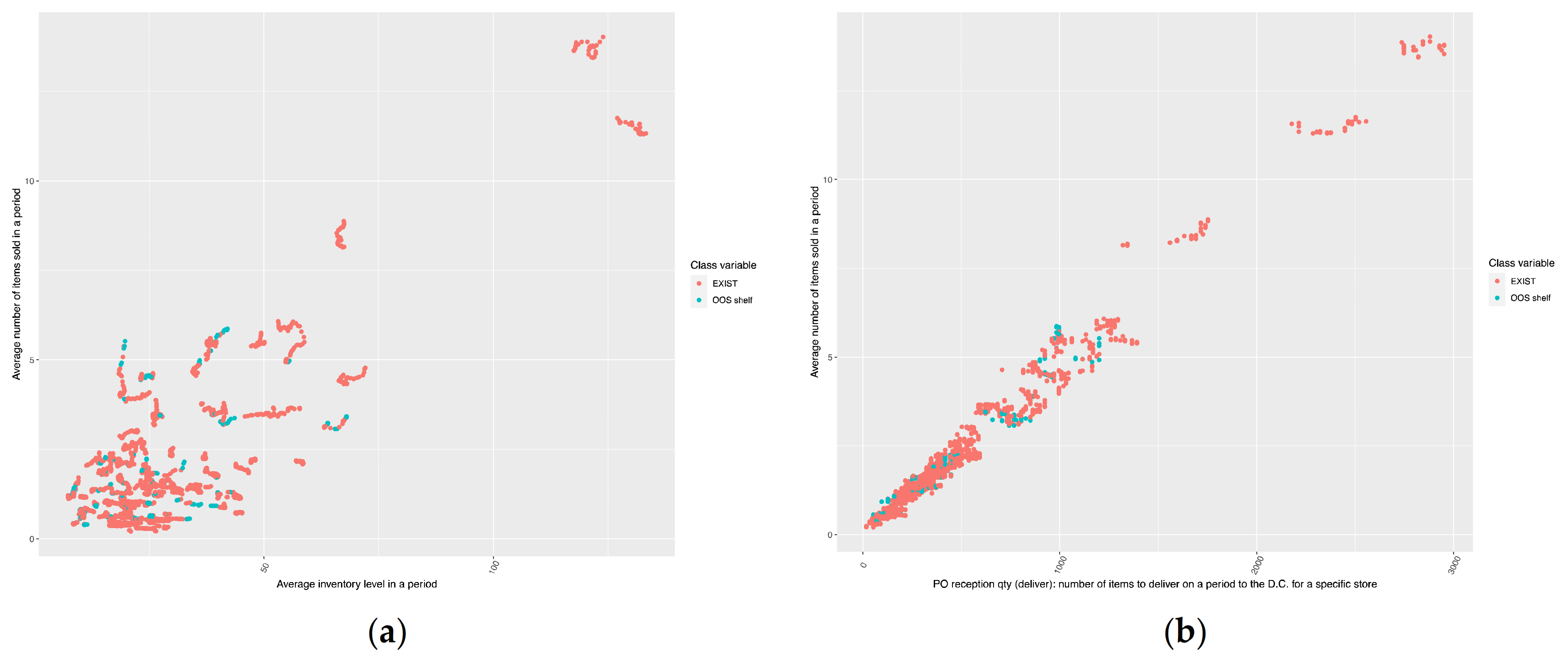
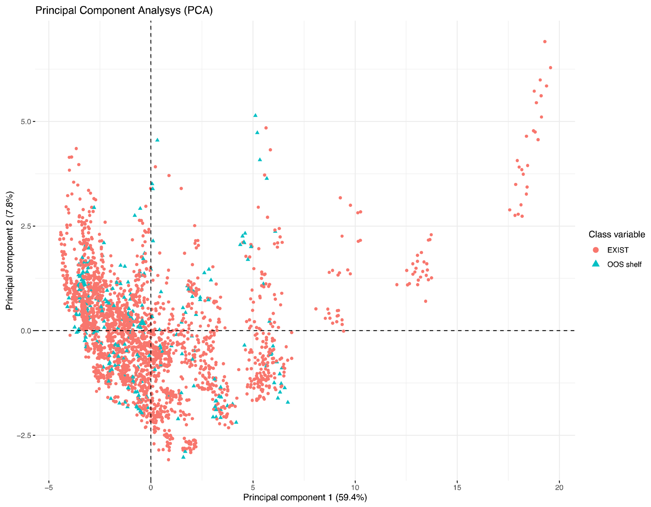
4.2. Data Set Construction and Exploratory Data Analysis (EDA)
4.3. Classification Algorithms Evaluation
4.4. Imbalance Data Problem
4.5. Machine Learning Based System implementation: Real-World Setting
5. Discussion
6. Conclusions
Author Contributions
Funding
Data Availability Statement
Conflicts of Interest
References
- García-Arca, J.; Prado-Prado, J.C.; González-Portela Garrido, A.T. On-shelf availability and logistics rationalization. A participative methodology for supply chain improvement. J. Retail. Consum. Serv. 2020, 52, 101889. [Google Scholar] [CrossRef]
- Mou, S.; Robb, D.J.; DeHoratius, N. Retail store operations: Literature review and research directions. Eur. J. Oper. Res. 2018, 265, 399–422. [Google Scholar] [CrossRef]
- Berger, R. Optimal Shelf Availability: Increasing Shopper Satisfaction at the Moment of Truth; Roland Berger Consultants: Kontich, Belgium, 2003; pp. 1–64. [Google Scholar]
- Corsten, D.; Gruen, T. Desperately seeking shelf availability: An examination of the extent, the causes, and the efforts to address retail out-of-stocks. Int. J. Retail Distrib. Manag. 2003, 31, 605–617. [Google Scholar] [CrossRef]
- Gruen, T.W.; Corsten, D. A Comprehensive Guide To Retail Reduction In the Fast-Moving Consumer Goods Industry; Grocery Manufacturers of America: Washington, DC, USA, 2008; ISBN 9783905613049. [Google Scholar]
- Buzek, G. Worldwide Costs of Retail Out-of-Stocks. Available online: https://www.ihlservices.com/news/analyst-corner/2018/06/worldwide-costs-of-retail-out-of-stocks/ (accessed on 1 June 2021).
- Papakiriakopoulos, D. Predict on-shelf product availability in grocery retailing with classification methods. Expert Syst. Appl. 2012, 39, 4473–4482. [Google Scholar] [CrossRef]
- Papakiriakopoulos, D.; Pramatari, K.; Doukidis, G. A decision support system for detecting products missing from the shelf based on heuristic rules. Decis. Support Syst. 2009, 46, 685–694. [Google Scholar] [CrossRef]
- Papakiriakopoulos, D. Developing a mechanism to support decisions for products missing from the shelf. J. Decis. Syst. 2011, 20, 417–441. [Google Scholar] [CrossRef]
- Chuang, H.H.C.; Oliva, R.; Liu, S. On-Shelf Availability, Retail Performance, and External Audits: A Field Experiment. Prod. Oper. Manag. 2016, 25, 935–951. [Google Scholar] [CrossRef]
- Montoya, R.; Gonzalez, C. A hidden Markov model to detect on-shelf out-of-stocks using point-of-sale data. Manuf. Serv. Oper. Manag. 2019, 21, 932–948. [Google Scholar] [CrossRef] [Green Version]
- Geng, Z.; Wang, Z.; Weng, T.; Huang, Y.; Zhu, Y. Shelf Product Detection Based on Deep Neural Network. In Proceedings of the 2019 12th International Congress on Image and Signal Processing, BioMedical Engineering and Informatics (CISP-BMEI), Suzhou, China, 19–21 October 2019; pp. 1–6. [Google Scholar]
- Mehta, R.N.; Joshi, H.V.; Dossa, I.; Gyanch Yadav, R.; Mane, S.; Rathod, M. Supermarket Shelf Monitoring Using ROS based Robot. In Proceedings of the 2021 5th International Conference on Trends in Electronics and Informatics (ICOEI), Tirunelveli, India, 3–5 June 2021; pp. 58–65. [Google Scholar]
- Craciunescu, M.; Baicu, D.; Mocanu, S.; Dobre, C. Determining on-shelf availability based on RGB and ToF depth cameras. In Proceedings of the 2021 23rd International Conference on Control Systems and Computer Science (CSCS), Bucharest, Romania, 26–28 May 2021; pp. 243–248. [Google Scholar]
- Chen, J.; Wang, S.-L.; Lin, H.-L. Out-of-Stock Detection Based on Deep Learning. In Proceedings of the 15th International Conference, ICIC 2019, Nanchang, China, 3–6 August 2019; pp. 228–237. [Google Scholar]
- Higa, K.; Iwamoto, K. Robust shelf monitoring using supervised learning for improving on-shelf availability in retail stores. Sensors 2019, 19, 2722. [Google Scholar] [CrossRef] [Green Version]
- Yilmazer, R.; Birant, D. Shelf auditing based on image classification using semi-supervised deep learning to increase on-shelf availability in grocery stores. Sensors 2021, 21, 327. [Google Scholar] [CrossRef]
- Avlijas, G.; Vukanovic Dumanovic, V.; Radunovic, M. Measuring the effects of automatic replenishment on product availability in retail stores. Sustainability 2021, 13, 1391. [Google Scholar] [CrossRef]
- Aastrup, J.; Kotzab, H. Forty years of Out-of-Stock research—And shelves are still empty. Int. Rev. Retail. Distrib. Consum. Res. 2010, 20, 147–164. [Google Scholar] [CrossRef]
- Moussaoui, I.; Williams, B.D.; Hofer, C.; Aloysius, J.A.; Waller, M.A. Drivers of retail on-shelf availability: Systematic review, critical assessment, and reflections on the road ahead. Int. J. Phys. Distrib. Logist. Manag. 2016, 46, 516–535. [Google Scholar] [CrossRef]
- Fitzsimons, G.J. Consumer response to stockouts. J. Consum. Res. 2000, 27, 249–266. [Google Scholar] [CrossRef]
- Koos, S.E.; Shaikh, N.I. Dynamics of Consumers’ Dissatisfaction Due to Stock-Outs. Int. J. Prod. Econ. 2019, 208, 461–471. [Google Scholar] [CrossRef]
- Azeem, M.M.; Baker, D.; Villano, R.A.; Mounter, S.; Griffith, G. Response to stockout in grocery stores: A small city case in a changing competitive environment. J. Retail. Consum. Serv. 2019, 49, 242–252. [Google Scholar] [CrossRef]
- Hamilton, R.; Thompson, D.; Bone, S.; Chaplin, L.N.; Griskevicius, V.; Goldsmith, K.; Hill, R.; John, D.R.; Mittal, C.; O’Guinn, T.; et al. The effects of scarcity on consumer decision journeys. J. Acad. Mark. Sci. 2019, 47, 532–550. [Google Scholar] [CrossRef]
- Verbeke, W.; Farris, P.; Thurik, R. Consumer response to the preferred brand out-of-stock situation. Eur. J. Mark. 1998, 32, 1008–1028. [Google Scholar] [CrossRef]
- Campo, K.; Gijsbrechts, E.; Nisol, P. Towards understanding consumer response to stock-outs. J. Retail. 2000, 76, 219–242. [Google Scholar] [CrossRef]
- Ehrenthal, J.C.F.; Stölzle, W. An examination of the causes for retail stockouts. Int. J. Phys. Distrib. Logist. Manag. 2013, 43, 54–69. [Google Scholar] [CrossRef]
- Andersen Consulting. The Retail Problem of Out-of-Stock Merchandise; Coca-Cola Retailing Research Council: Atlanta, Georgia, 1996. [Google Scholar]
- Kang, Y.; Gershwin, S.B. Information inaccuracy in inventory systems: Stock loss and stockout. IIE Trans. 2005, 37, 843–859. [Google Scholar] [CrossRef]
- Frontoni, E.; Marinelli, F.; Rosetti, R.; Zingaretti, P. Shelf space re-allocation for out of stock reduction. Comput. Ind. Eng. 2017, 106, 32–40. [Google Scholar] [CrossRef]
- Reiner, G.; Teller, C.; Kotzab, H. Analyzing the efficient execution of in-store logistics processes in grocery retailing—The case of dairy products. Prod. Oper. Manag. 2013, 22, 924–939. [Google Scholar] [CrossRef] [Green Version]
- Condea, C.; Thiesse, F.; Fleisch, E. RFID-enabled shelf replenishment with backroom monitoring in retail stores. Decis. Support Syst. 2012, 52, 839–849. [Google Scholar] [CrossRef]
- Rosales, C.R.; Whipple, J.M.; Blackhurst, J. The Impact of Distribution Channel Decisions and Repeated Stockouts on Manufacturer and Retailer Performance. IEEE Trans. Eng. Manag. 2019, 66, 312–324. [Google Scholar] [CrossRef]
- Avlijas, G.; Simicevic, A.; Avlijas, R.; Prodanovic, M. Measuring the impact of stock-keeping unit attributes on retail stock-out performance. Oper. Manag. Res. 2015, 8, 131–141. [Google Scholar] [CrossRef]
- Williams, B.D.; Waller, M.A.; Ahire, S.; Ferrier, G.D. Predicting retailer orders with POS and order data: The inventory balance effect. Eur. J. Oper. Res. 2014, 232, 593–600. [Google Scholar] [CrossRef]
- Chen, C.Y.; Lee, W.I.; Kuo, H.M.; Chen, C.W.; Chen, K.H. The study of a forecasting sales model for fresh food. Expert Syst. Appl. 2010, 37, 7696–7702. [Google Scholar] [CrossRef]
- Waller, M.A.; Williams, B.D.; Tangari, A.H.; Burton, S. Marketing at the retail shelf: An examination of moderating effects of logistics on SKU market share. J. Acad. Mark. Sci. 2010, 38, 105–117. [Google Scholar] [CrossRef]
- Fisher, M.; Raman, A. The New Science of Retailing; Harvard Business Review Press: Cambridge, MA, USA, 2010; ISBN 9781422110577. [Google Scholar]
- Bottani, E.; Bertolini, M.; Rizzi, A.; Romagnoli, G. Monitoring on-shelf availability, out-of-stock and product freshness through RFID in the fresh food supply chain. Int. J. RF Technol. Res. Appl. 2017, 8, 33–55. [Google Scholar] [CrossRef]
- Metzger, C.; Thiesse, F.; Gershwin, S.; Fleisch, E. The impact of false-negative reads on the performance of RFID-based shelf inventory control policies. Comput. Oper. Res. 2013, 40, 1864–1873. [Google Scholar] [CrossRef]
- Mersereau, A.J. Demand estimation from censored observations with inventory record inaccuracy. Manuf. Serv. Oper. Manag. 2015, 17, 335–349. [Google Scholar] [CrossRef] [Green Version]
- Sarac, A.; Absi, N.; Dauzere-Pérès, S. A literature review on the impact of RFID technologies on supply chain management. Int. J. Prod. Econ. 2010, 128, 77–95. [Google Scholar] [CrossRef]
- Piramuthu, S.; Wochner, S.; Grunow, M. Should retail stores also RFID-tag “cheap” items? Eur. J. Oper. Res. 2014, 233, 281–291. [Google Scholar] [CrossRef]
- Franco, A.; Maltoni, D.; Papi, S. Grocery product detection and recognition. Expert Syst. Appl. 2017, 81, 163–176. [Google Scholar] [CrossRef]
- Fleisch, E.; Tellkamp, C. Inventory inaccuracy and supply chain performance: A simulation study of a retail supply chain. Int. J. Prod. Econ. 2005, 95, 373–385. [Google Scholar] [CrossRef]
- Chen, L. Fixing Phantom Stockouts: Optimal Data-Driven Shelf Inspection Policies. SSRN Electron. J. 2015, 1–21. [Google Scholar] [CrossRef] [Green Version]
- Chuang, H.H.C. Fixing shelf out-of-stock with signals in point-of-sale data. Eur. J. Oper. Res. 2018, 270, 862–872. [Google Scholar] [CrossRef]
- R Core Team. R: A Language and Environment for Statistical Computing; R Foundation for Statistical Computing: Vienna, Austria, 2020. [Google Scholar]
- Kassambara, A.; Mundt, F. factoextra: Extract and Visualize the Results of Multivariate Data Analyses, R package version 1.0.7; R Foundation for Statistical Computing: Vienna, Austria, 2020; Available online: https://CRAN.R-project.org/package=factoextra (accessed on 1 June 2021).
- Dimitriadou, E.; Hornik, K.; Leisch, F.; Meyer, D.; Weingessel, A. e1071: Misc Functions of them Department of Statistics, Probability Theory Group (Formerly: E1071), R package version 1.7-4; R Foundation for Statistical Computing: Vienna, Austria, 2020; Available online: https://CRAN.R-project.org/package=e1071 (accessed on 1 June 2021).
- Hothorn, T.; Hornik, K.; Zeileis, A. Unbiased Recursive Partitioning: A Conditional Inference Framework. J. Comput. Graph. Stat. 2006, 15, 651–674. [Google Scholar] [CrossRef] [Green Version]
- Wright, M.N.; Ziegler, A. ranger: A Fast Implementation of Random Forests for High Dimensional Data in C++ and R. J. Stat. Softw. 2017, 77, 1–17. [Google Scholar] [CrossRef] [Green Version]
- Venables, W.N.; Ripley, B.D. Modern Applied Statistics with R, 4th ed.; Springer: New York, NY, USA, 2002; ISBN 0-387-95457-0. [Google Scholar]
- Kuhn, M. Caret: Classification and Regression Training, R package version 6.0-86; R Foundation for Statistical Computing: Vienna, Austria, 2020; Available online: https://CRAN.R-project.org/package=caret (accessed on 1 June 2021).
- Polikar, R. Ensemble based systems in decision making. IEEE Circuits Syst. Mag. 2006, 6, 21–44. [Google Scholar] [CrossRef]
- Sasaki, Y. The truth of the F-measure. Teach Tutor Mater. 2007, 1, 1–5. [Google Scholar]
- Lunardon, N.; Menardi, G.; Torelli, N. ROSE: A Package for Binary Imbalanced Learning. R. J. 2014, 6, 82–92. [Google Scholar] [CrossRef] [Green Version]
- Gruen, T.W.; Corsten, D.S.; Bharadwaj, S. Retail Out-of-Stocks: A Worldwide Examination of Causes, Rates, and Consumer Responses; Grocery Manufacturers of America: Washington, DC, USA, 2002. [Google Scholar]
- Das, S.; Datta, S.; Chaudhuri, B.B. Handling data irregularities in classification: Foundations, trends, and future challenges. Pattern Recognit. 2018, 81, 674–693. [Google Scholar] [CrossRef]


| DS.Initial | DS.CS_1 | DS.CS_2 | ||||
|---|---|---|---|---|---|---|
| Attribute Category | Attribute Description | Attribute Name | Predictor Variables Selection | Predictor Variables Selection | Predictor Variables Source | References |
| Sales features | Items sold for the specific day | SF 1 | YES | YES | Information system | [7,8] |
| Average number of items sold in a period | SF 2 | YES | YES | Computed | [7,8] | |
| Standard deviation of items sold in a period | SF 3 | YES | YES | Computed | [7,8] | |
| Average items sold for a specific day of the week in a period | SF 4 | YES | YES | Computed | [7,8] | |
| Standard deviation of items sold for a specific day of the week in a period | SF 5 | YES | YES | Computed | [7,8] | |
| Average number of sales using only the days that a product made a sale in a period | SF 6 | YES | YES | Computed | [7,8] | |
| Standard deviation of sales using only the days that a product made a sale in a period | SF 7 | YES | YES | Computed | [7,8] | |
| The number of days that a product hasn’t sold any single unit in a period | SF 8 | YES | YES | Computed | [7,8] | |
| The average number of days that the product is not selling a unit | SF 9 | YES | YES | Computed | [7,8] | |
| The standard deviation of days that the product is not selling a unit | SF 10 | YES | YES | Computed | [7,8] | |
| The number of days that a product hasn´t sold any single unit in a period/Total number of days in a period (percent) | SF 11 | YES | YES | Computed | New attribute | |
| The total number of days that a product hasn´t sold any single unit in a period | SF 12 | YES | YES | Computed | New attribute | |
| Median number of items sold in a period | SF 13 | YES | YES | Computed | New attribute | |
| Items sold for the specific day/Average number of items sold in a period (percent) | SF 14 | YES | YES | Computed | New attribute | |
| Inventory features | Inventory level for the specific day | IF 1 | NO | YES | Information system | New attribute |
| Inventory level for the specific day before | IF 2 | NO | YES | Computed | New attribute | |
| Average inventory level in a period | IF 3 | NO | YES | Computed | New attribute | |
| Standard deviation inventory level in a period | IF 4 | NO | YES | Computed | New attribute | |
| Average inventory level for a specific day of the week in a period | IF 5 | NO | YES | Computed | New attribute | |
| Standard deviation inventory level for a specific day of the week in a period | IF 6 | NO | YES | Computed | New attribute | |
| Average inventory level using only the days that a product has positive stock in a period | IF 7 | NO | YES | Computed | New attribute | |
| Standard deviation inventory level using only the days that a product has positive stock in a period | IF 8 | NO | YES | Computed | New attribute | |
| In stock for the specific day | IF 9 | NO | YES | Information system | New attribute | |
| Stock adjustment for the specific day | IF 10 | NO | YES | Information system | New attribute | |
| Average Stock adjustment in a period | IF 11 | NO | YES | Computed | New attribute | |
| Standard deviation Stock adjustment in a period | IF 12 | NO | YES | Computed | New attribute | |
| Average Stock adjustment for a specific day of the week in a period | IF 13 | NO | YES | Computed | New attribute | |
| Standard deviation Stock adjustment for a specific day of the week in a period | IF 14 | NO | YES | Computed | New attribute | |
| The number of days that a product has been adjusted in a period | IF 15 | NO | YES | Computed | New attribute | |
| The number of days that a product has been adjusted in a period/Total number of days in a period (percent) | IF 16 | NO | YES | Computed | New attribute | |
| The number of days that a product has been positive adjusted in a period | IF 17 | NO | YES | Computed | New attribute | |
| The number of days that a product has been positive adjusted in a period/Total number of days in a period (percent) | IF 18 | NO | YES | Computed | New attribute | |
| The number of days that a product has been negative adjusted in a period | IF 19 | NO | YES | Computed | New attribute | |
| The number of days that a product has been negative adjusted in a period/Total number of days in a period (percent) | IF 20 | NO | YES | Computed | New attribute | |
| Product features | The product is a regular line product or a promotional item | PF 1 | NO | NO | Information system | [7,8] |
| The product is new or regular | PF 2 | NO | NO | Information system | [7,8] | |
| Product category | PF 3 | NO | NO | Information system | [7,8] | |
| Product subcategory | PF 4 | NO | NO | Information system | [7,8] | |
| Product Shelf Life | PF 5 | NO | NO | Information system | New attribute | |
| Product Status | PF 6 | NO | NO | Information system | New attribute | |
| Context features | The size of the store | CF 1 | YES | YES | Information system | [7,8] |
| The day of the week | CF 2 | YES | YES | Information system | [7,8] | |
| Moving index | CF 3 | YES | YES | Computed | [7,8] | |
| Supply Chain features | The logistics method for the specific product in the specific store (Product distribution) | SC 1 | NO | NO | Information system | New attribute |
| The replenishment method for the specific product in the specific store (Product replenishment) | SC 2 | NO | NO | Information system | [7,8] | |
| Ordering features | PO emission: number of items purchased on a specific day in the specific store | OF 1 | NO | YES | Information system | New attribute |
| Average PO emission in a period | OF 2 | NO | YES | Computed | New attribute | |
| Standard deviation PO emission in a period | OF 3 | NO | YES | Computed | New attribute | |
| Average PO emission for a specific day of the week in a period | OF 4 | NO | YES | Computed | New attribute | |
| Standard deviation PO emission for a specific day of the week in a period | OF 5 | NO | YES | Computed | New attribute | |
| PO reception qty (deliver): number of items to deliver on a specific day to the DC for a specific store | OF 6 | NO | YES | Information system | New attribute | |
| PO reception qty (received): number of items received on a specific day to the DC for a specific store | OF 7 | NO | YES | Information system | New attribute | |
| Fill rate percent: number of item received/number of items purchased on a specific day in the specific store | OF 8 | NO | YES | Computed | New attribute | |
| Fill rate percent in a period | OF 9 | NO | YES | Computed | New attribute | |
| Average PO emission last 14 days | OF 10 | NO | YES | Computed | New attribute | |
| Standard deviation PO last 14 days | OF 11 | NO | YES | Computed | New attribute | |
| Fill rate percent last 14 days | OF 12 | NO | YES | Computed | New attribute | |
| The number of days that a product has been ordered in a period | OF 13 | NO | YES | Computed | New attribute | |
| The number of days that a product has been ordered in a period/Total number of days in a period (percent) | OF 14 | NO | YES | Computed | New attribute | |
| PO reception qty (deliver): number of items to deliver on a period to the DC for a specific store | OF 15 | NO | YES | Computed | New attribute | |
| PO reception qty (received): number of items received on a period to the DC for a specific store | OF 16 | NO | YES | Computed | New attribute | |
| Description features | Product number | DI 1 | NO | NO | Information system | |
| Product description | DI 2 | NO | NO | Information system | ||
| Store number | DI 3 | NO | NO | Information system | ||
| Store description | DI 4 | NO | NO | Information system | ||
| Date | DI 5 | NO | NO | Information system | ||
| PO emission number | DI 6 | |||||
| PO reception number | DI 7 | NO | NO | Information system | ||
| Total number of attributes per datasets | 68 | 13 | 53 | |||
| Actual | |||
|---|---|---|---|
| OOS Shelf | EXIST | ||
| Prediction | OOS Shelf | True Positive (TP) | False Negative (FN) |
| EXIST | False Positive (FP) | True Negative (TN) | |
| Dataset | Description | Observed Class | Total | Rate | Category | Product Characteristics | |
|---|---|---|---|---|---|---|---|
| EXIST | OOS | EXIST + OOS | OOS | ||||
| Pa.D | Store physical audit dataset | 2948 | 327 | 3275 | 10.0% | Fresh fruits and vegetables | Non-perishable food (Nuts and Dried fruit) |
| DS.CS_1 | DS.CS_2 | ||||||||||||
|---|---|---|---|---|---|---|---|---|---|---|---|---|---|
| Accuracy | Sensitivity | Pos. Pred. value | Specificity | Neg. Pred. value | F-measure | Accuracy | Sensitivity | Pos. Pred. value | Specificity | Neg. Pred. value | F-measure | ||
| Random Forest | mean | 0.91371 | 0.24164 | 0.73593 | 0.98991 | 0.92012 | 0.36381 | 0.93483 | 0.46179 | 0.85182 | 0.99054 | 0.93989 | 0.59890 |
| sd | 0.00845 | 0.03856 | 0.08690 | 0.00424 | 0.00872 | 0.05341 | 0.00909 | 0.05364 | 0.05610 | 0.00385 | 0.00962 | 0.05484 | |
| Logistics Regression | mean | 0.89786 | 0.00998 | 0.33848 | 0.99834 | 0.89910 | 0.01939 | 0.89378 | 0.11894 | 0.48455 | 0.98479 | 0.90493 | 0.19100 |
| sd | 0.00811 | 0.01016 | 0.33726 | 0.00142 | 0.00817 | 0.01972 | 0.01066 | 0.03310 | 0.11306 | 0.00553 | 0.01061 | 0.05121 | |
| Decision Tree | mean | 0.89719 | 0.10076 | 0.44402 | 0.98739 | 0.90657 | 0.16425 | 0.89838 | 0.27292 | 0.53902 | 0.97196 | 0.91924 | 0.36236 |
| sd | 0.00858 | 0.05844 | 0.16184 | 0.00737 | 0.00968 | 0.08587 | 0.01099 | 0.07337 | 0.09683 | 0.00997 | 0.01194 | 0.08348 | |
| Naïve Bayes | mean | 0.84537 | 0.19484 | 0.22353 | 0.91909 | 0.90979 | 0.20820 | 0.49551 | 0.70547 | 0.13648 | 0.47089 | 0.93096 | 0.22871 |
| sd | 0.01885 | 0.03041 | 0.05639 | 0.02300 | 0.00782 | 0.03951 | 0.05285 | 0.04651 | 0.01934 | 0.06058 | 0.01383 | 0.02732 | |
| radial Support Vector Machines | mean | 0.89768 | 0.02031 | 0.46870 | 0.99701 | 0.89990 | 0.03893 | 0.89718 | 0.03019 | 0.77800 | 0.99900 | 0.89767 | 0.05812 |
| sd | 0.00829 | 0.01287 | 0.28384 | 0.00244 | 0.00849 | 0.02461 | 0.01046 | 0.01397 | 0.26620 | 0.00121 | 0.01081 | 0.02655 | |
| Neural Networks | mean | 0.89943 | 0.07371 | 0.55110 | 0.99293 | 0.90447 | 0.13003 | 0.89631 | 0.13215 | 0.53547 | 0.98603 | 0.90640 | 0.21199 |
| sd | 0.00853 | 0.02628 | 0.13326 | 0.00311 | 0.00865 | 0.04391 | 0.01102 | 0.06019 | 0.17137 | 0.00902 | 0.01110 | 0.08909 | |
| Ensemble (stacking-linear regression) | mean | 0.91667 | 0.31467 | 0.70757 | 0.98497 | 0.92689 | 0.43561 | 0.93967 | 0.56735 | 0.80480 | 0.98358 | 0.95072 | 0.66553 |
| sd | 0.00844 | 0.04419 | 0.07698 | 0.00534 | 0.00874 | 0.05615 | 0.00880 | 0.05451 | 0.05792 | 0.00590 | 0.00901 | 0.05616 | |
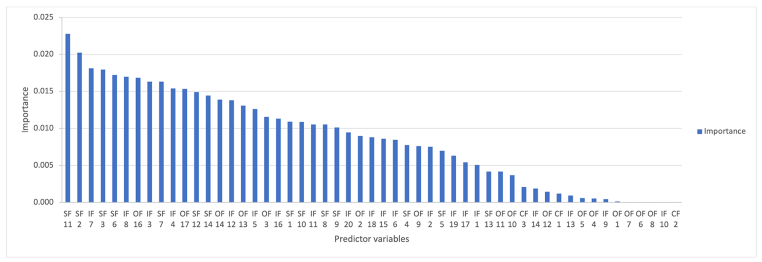
| Predictor Variables | Attribute Description | Importance | Rank | References |
|---|---|---|---|---|
| SF 11 | The number of days that a product has not sold any single unit in a period/Total number of days in a period (percent) | 0.02280 | 1 | New attribute |
| SF 2 | Average number of items sold in a period | 0.02022 | 2 | [7,8] |
| IF 7 | Average inventory level using only the days that a product has positive stock in a period | 0.01811 | 3 | New attribute |
| SF 3 | Standard deviation of items sold in a period | 0.01793 | 4 | [7,8] |
| SF 6 | Average number of sales using only the days that a product made a sale in a period | 0.01721 | 5 | [7,8] |
| IF 8 | Standard deviation inventory level using only the days that a product has positive stock in a period | 0.01700 | 6 | New attribute |
| OF 16 | PO reception qty (deliver): number of items to deliver on a period to the D.C. for a specific store | 0.01685 | 7 | New attribute |
| IF 3 | Average inventory level in a period | 0.01634 | 8 | New attribute |
| SF 7 | Standard deviation of sales using only the days that a product made a sale in a period | 0.01632 | 9 | [7,8] |
| IF 4 | Standard deviation inventory level in a period | 0.01540 | 10 | New attribute |
| OF 17 | PO reception qty (received): number of items received on a period to the D.C. for a specific store | 0.01534 | 11 | New attribute |
| SF 12 | The number of days that a product hasn’t sold any single unit in a period | 0.01491 | 12 | New attribute |
| SF 14 | Items sold for the specific day/Average number of items sold in a period (percent) | 0.01445 | 13 | New attribute |
| OF 14 | The number of days that a product has been ordered in a period/Total number of days in a period (percent) | 0.01389 | 14 | New attribute |
| IF 12 | Standard deviation Stock adjustment in a period | 0.01381 | 15 | New attribute |
| Dataset | Statistics | Random Forest | |||||
|---|---|---|---|---|---|---|---|
| Accuracy | Sensitivity | Pos. Pred. Value | Specificity | Neg. Pred. Value | F-Measure | ||
| Not Balanced Data DS.CS_2 | mean | 0.93430 | 0.46316 | 0.85453 | 0.99058 | 0.93924 | 0.60073 |
| sd | 0.00850 | 0.05119 | 0.05436 | 0.00383 | 0.00912 | 0.05273 | |
| Balanced Data Oversampling 20% | mean | 0.93457 | 0.50002 | 0.81394 | 0.98628 | 0.94317 | 0.61948 |
| sd | 0.00827 | 0.05927 | 0.06509 | 0.00538 | 0.00853 | 0.06204 | |
| Balanced Data Oversampling 30% | mean | 0.93608 | 0.56350 | 0.77449 | 0.98045 | 0.94973 | 0.65236 |
| sd | 0.00831 | 0.06287 | 0.05794 | 0.00560 | 0.00869 | 0.06030 | |
| Balanced Data Oversampling 40% | mean | 0.93650 | 0.58342 | 0.76570 | 0.97855 | 0.95182 | 0.66225 |
| sd | 0.00804 | 0.05603 | 0.06268 | 0.00669 | 0.00795 | 0.05917 | |
| Balanced Data Oversampling 50% | mean | 0.93530 | 0.58124 | 0.75573 | 0.97750 | 0.95150 | 0.65710 |
| sd | 0.00853 | 0.06036 | 0.06206 | 0.00665 | 0.00862 | 0.06120 | |
| Balanced Data Oversampling 20% | mean | 0.92662 | 0.57491 | 0.68717 | 0.96841 | 0.95049 | 0.62605 |
| sd | 0.00926 | 0.06244 | 0.06812 | 0.00911 | 0.00808 | 0.06515 | |
| Balanced Data Oversampling 30% | mean | 0.90437 | 0.66823 | 0.54283 | 0.93247 | 0.95948 | 0.59904 |
| sd | 0.01205 | 0.06372 | 0.05755 | 0.01327 | 0.00842 | 0.06048 | |
| Balanced Data Oversampling 40% | mean | 0.86063 | 0.75208 | 0.41646 | 0.87361 | 0.96742 | 0.53607 |
| sd | 0.01772 | 0.06137 | 0.04482 | 0.02103 | 0.00842 | 0.05181 | |
| Balanced Data Oversampling 50% | mean | 0.78274 | 0.82056 | 0.30694 | 0.77814 | 0.97351 | 0.44676 |
| sd | 0.02543 | 0.05332 | 0.03150 | 0.03011 | 0.00741 | 0.03960 | |
| Dataset | Statistics | Ensemble | |||||
|---|---|---|---|---|---|---|---|
| Accuracy | Sensitivity | Pos. Pred. Value | Specificity | Neg. Pred. Value | F-Measure | ||
| Not Balanced Data DS.CS_2 | mean | 0.93967 | 0.56735 | 0.80480 | 0.98358 | 0.95072 | 0.66553 |
| sd | 0.00880 | 0.05451 | 0.05792 | 0.00590 | 0.00901 | 0.05616 | |
| Balanced Data Oversampling 20% | mean | 0.93123 | 0.44123 | 0.82372 | 0.98863 | 0.93801 | 0.57465 |
| sd | 0.00971 | 0.06576 | 0.06237 | 0.00510 | 0.01100 | 0.06402 | |
| Balanced Data Oversampling 30% | mean | 0.92754 | 0.39072 | 0.82858 | 0.99031 | 0.71529 | 0.53103 |
| sd | 0.01015 | 0.07590 | 0.06494 | 0.00465 | 0.40148 | 0.06999 | |
| Balanced Data Oversampling 40% | mean | 0.91935 | 0.26699 | 0.87367 | 0.99547 | 0.92093 | 0.40899 |
| sd | 0.01105 | 0.05479 | 0.07258 | 0.00269 | 0.01076 | 0.06244 | |
| Balanced Data Oversampling 50% | mean | 0.90772 | 0.12876 | 0.90673 | 0.99864 | 0.90767 | 0.22550 |
| sd | 0.01291 | 0.06572 | 0.13297 | 0.00197 | 0.01254 | 0.08796 | |
| Balanced Data Oversampling 20% | mean | 0.92604 | 0.61306 | 0.66034 | 0.96262 | 0.95522 | 0.63582 |
| sd | 0.00957 | 0.06414 | 0.05996 | 0.01010 | 0.00896 | 0.06198 | |
| Balanced Data Oversampling 30% | mean | 0.89986 | 0.70397 | 0.51847 | 0.92288 | 0.96383 | 0.59714 |
| sd | 0.01580 | 0.05737 | 0.06056 | 0.01619 | 0.00864 | 0.05892 | |
| Balanced Data Oversampling 40% | mean | 0.85877 | 0.76567 | 0.40731 | 0.86970 | 0.96946 | 0.53174 |
| sd | 0.01623 | 0.04774 | 0.03135 | 0.01833 | 0.00753 | 0.03784 | |
| Balanced Data Oversampling 50% | mean | 0.81420 | 0.81740 | 0.34075 | 0.81412 | 0.97430 | 0.48099 |
| sd | 0.02507 | 0.04362 | 0.03980 | 0.02811 | 0.00760 | 0.04162 | |
| Stages: | Stage 1 | Stage 2 | Stage 3 | Stage 4 | Stage 5 | Stage 6 |
|---|---|---|---|---|---|---|
| Activity: | Daily POS data extraction and consolidation from the manufacturer´s IS | Data processing | Computation of Predictor variables | OOS prediction | Preparation of daily reports for the manufacturer´s store visitors’ staff | Store visits to correct potential OOS events |
| Resource: | IT staff | IT staff | IT staff | IT staff | IT staff | Store visitors’ staff |
| Dataset | Description | Observed Class | Total | Rate | Category | Product Characteristics | |
|---|---|---|---|---|---|---|---|
| EXIST | OOS | EXIST + OOS | OOS | ||||
| Pa.D_Val | Store physical audit dataset: Machine Learning system validation | 1713 | 51 | 1764 | 2.9% | Fresh fruits and vegetables | Non-perishable food (Nuts and Dried fruit) |
| DETECTION SYSTEM | Performance Metrics | ||
|---|---|---|---|
| Sensitivity | Pos. Pred. Value | F-Measure | |
| Machine Learning based system: Real-world OOS prediction (Ensemble) | 0.58000 | 0.77333 | 0.66286 |
| Machine Learning based system: Real-world OOS prediction (Random Forest) | 0.68000 | 0.72340 | 0.70103 |
Publisher’s Note: MDPI stays neutral with regard to jurisdictional claims in published maps and institutional affiliations. |
© 2021 by the authors. Licensee MDPI, Basel, Switzerland. This article is an open access article distributed under the terms and conditions of the Creative Commons Attribution (CC BY) license (https://creativecommons.org/licenses/by/4.0/).
Share and Cite
Andaur, J.M.R.; Ruz, G.A.; Goycoolea, M. Predicting Out-of-Stock Using Machine Learning: An Application in a Retail Packaged Foods Manufacturing Company. Electronics 2021, 10, 2787. https://doi.org/10.3390/electronics10222787
Andaur JMR, Ruz GA, Goycoolea M. Predicting Out-of-Stock Using Machine Learning: An Application in a Retail Packaged Foods Manufacturing Company. Electronics. 2021; 10(22):2787. https://doi.org/10.3390/electronics10222787
Chicago/Turabian StyleAndaur, Juan Manuel Rozas, Gonzalo A. Ruz, and Marcos Goycoolea. 2021. "Predicting Out-of-Stock Using Machine Learning: An Application in a Retail Packaged Foods Manufacturing Company" Electronics 10, no. 22: 2787. https://doi.org/10.3390/electronics10222787
APA StyleAndaur, J. M. R., Ruz, G. A., & Goycoolea, M. (2021). Predicting Out-of-Stock Using Machine Learning: An Application in a Retail Packaged Foods Manufacturing Company. Electronics, 10(22), 2787. https://doi.org/10.3390/electronics10222787