Methodology of Adaptive Instantaneous Overcurrent Protection Setting

Abstract

This paper proposed a methodology of adaptive instantaneous overcurrent protection (AIOCP) setting that ensures that the protection coverage remains unchanged regardless of the operating condition of the electrical network. The methodology calculates the protection setting parameters based on the real-time estimation of the Thevenin equivalent circuit (TEC). The estimation algorithm uses the positive-sequence voltage and current values and a system of non-linear equations, which is solved iteratively by the Gauss–Newton method. The proposed methodology calculates the IOCP settings in real time by using the real-time estimation of the TEC; therefore, any change in the electric network conditions is represented in the TEC, and the calculated setting keeps the desired protection coverage constant. Simulation results demonstrate that the proposed AIOCP can keep constant the protection coverage overcoming the classical problems of classical IOCP: sub-allocation and over-coverage.

1. Introduction

1.1. Motivation

The ultimate goal of an overcurrent (OC) protective system is to disconnect a faulty system element (or elements) as quickly as possible so that the impact on the rest of the system is minimised and as much as possible is left intact. The OC protection (OCP) is directed entirely to the clearance of faults, short circuits.

Five functional characteristics define the performance of the protection system [1]: reliability, selectivity, speed, cost, and simplicity. The selectivity can be achieved with “inherently selective” devices, which means the device operates only on faults within its “zone of protection” and does not ordinarily sense faults outside that zone. The sensitivity, together with the selectivity, is vital to assure that the proper circuit breakers will be tripped, but speed is the “pay-off” [1].

Two main methods achieve the selectivity of OCP: (i) time-grading/current grading: relays are set to operate depending on the time and current characteristics, OCP coordination, and (ii) unit protection principle: current is measured at several points and compared, the fundamental element of the differential protection scheme.

OCP coordination (OCPC) objectives are to determine the characteristics, ratings, and settings of OCP devices that minimise equipment damage and interrupt short circuits as rapidly as possible. There are various possible methods used to achieve correct OC relay coordination (for primary and backup protection) [2], but all use discrimination either by time, overcurrent, or a combination of both. The appropriate instantaneous OC (IOC) relay coordination requires knowledge of the fault currents that can flow in each part of the network, as well as an adequate understanding of the operation and the characteristic curve of the OC relay. The momentary short-circuit currents (I_kss) are used to determine the maximum and minimum currents instantaneous trip devices respond to.

One of the significant disadvantages of OCP is the explicit dependence of the short-circuit currents to the source impedance variations. As a consequence, there is a loss of protection selectivity, which negatively affects the reliability of service to the loads provided by the network.

The most fundamental principle involved in determining the magnitude of short-circuit current is Ohm’s Law, which defines the fault current measured by IOC. The Thevenin equivalent (TE) model behind the protection is used to calculate the short-circuit currents in large power systems systematically. However, the TE impedance (TEI, sometimes called the driving-point impedance, Z_th) and the TE voltage (V_th) dynamically change during the system operation. The changes in the TE model parameters (V_th and Z_th) depend on many factors, such as the type and location of the fault, the topology of the electrical network, and the operating regime of generators, among others [3]. As the value of the TE model parameter changes, the fault current measured by the IOC protection changes.

The main impact of the changes in momentary short-circuit currents is on “the coverage areas” of the instantaneous OCPs. This is because the coverage of the IOCP is not constant and that they increase or decrease depending on the operating conditions of the electrical network before the fault occurs. Traditionally, the IOC protection of a distribution line is set between 80 and 90% of the line length to avoid problems of protection coordination with the IOC protections of the adjacent lines, but this practice could fail in modern active distribution networks.

This paper proposes a methodology of adaptive instantaneous overcurrent protection (AIOCP) setting that ensures that the protection coverage remains unchanged regardless of the operating condition of the power system, based only on positive-sequence voltage and current measurements. The proposed methodology is based on the estimation of the parameters of the TE model (TEM) in real time. It ensures the IOC protection settings are immune to the system changes and the maximum coverage area. Real-time implementation of the proposed methodology is not included in this paper.

1.2. Literature Review

The concept of adaptive protection is nothing new, but the actual implementation is relatively new [4]. However, the adaptive capability was very limited in old electromechanically and solid-state analogic systems. Later technological development made possible the full progress of the adaptive concept in OCP schemes. The literature related to adaptive OCP could be divided into two main categories, in historical sequence: (i) the traditional passive electric networks and (ii) active distribution systems, including distributed generation (DG).

Pioneering schemes of the adaptive overcurrent protection can be found in [5], where Rockefeller et al. propose the adaptive sequential instantaneous tripping but the installation of a multi-pilot scheme. The development of the classical adaptive OCP schemes is found mainly in the late 1980s and early 1990s. The primary focus was the development of the computer overcurrent relaying concept for distribution [6,7,8,9]. The idea of adaptive coordination of overcurrent relays in an interconnected power system using directional overcurrent relays is presented in [10]. A time overcurrent adaptive relay is proposed by Vazquez et al. in [11]. The modern era of adaptive OCP is marked by the rise of active distribution systems with DG in the early 2000s. The modern adaptive OCP is developed using the advances of digital technology and advanced algorithms: agent-based [12], adaptive fuzzy [13], adaptive network, and fuzzy inference systems [14]; Q-learning-based cooperative multi-agent systems [15]; and multi-agents [16].

Two OCP schemes using the locally available information to update relay settings are put forward in [17,18]. Another method to improve the functionality of the OC relay based on local measurements is described in [19]. These adaptive protection methods mainly focus on inverse-time OC protection.

The online TE is analysed in [20], a method with unsynchronised data considering measurement errors. Use of the synchrophasor voltage and current measurements from PMU is proposed in [21] for TE estimation. An adaptive algorithm for IOC relays based on frequency estimation is introduced in [22,23] describes a definite-time OC protection applied to the ungrounded distribution system. An online Thevenin equivalent circuit was employed to calculate varying short-circuit currents regarding any change in the grid [24], where the initial conditions were evaluated with a power flow analysis.

1.3. Contributions

This paper proposes a new methodology of adaptive instantaneous overcurrent protection (AIOCP) independent of the distribution electrical network configuration and operating regime of generators behind the protective relay. Consequently, the AIOCP is immune to sub-location and over-coverage; therefore, relay coverage remains constant (demonstrated in Section 5). Simulation results demonstrate the AIOCP could be adjusted without overlap with the coverage zone of the relay in the next line.

The AIOCP is based on real-time estimation of the Thevenin equivalent circuit (formulation presented in Section 3). It uses incremental signals to eliminate the steady-state components, making fault detection function immune to harmonics [25], which are common in distribution networks due to non-linear load and power electronic converters. Real-time implementation of the proposed methodology is outside the scope of this scientific paper.

1.4. Paper Organisation

The paper is structured into five sections: Section 1 presents the problem to be solved and the purpose of the article. A description of the instantaneous overcurrent protection is given in Section 2. The explanation of the proposed AIOCP is made in Section 3. The test system employed and simulations results are presented in Section 4, and Section 5 offers the conclusions of the paper.

2. Instantaneous Overcurrent Relay: Problem Formulation

OC relaying is the most straightforward and cheapest protection scheme, but it is the most difficult to apply and the quickest to need readjustment or even replacement as the power system changes. The operating principle of the OC relay (OCR) is based on the change in the current measured by the protection.

The IOC or a definite-time overcurrent (DTOC), ANSI device number 50, operates as soon as the current (I_meas) becomes higher than a pre-set value (I_pick). It has no intentional time delay set, but there is always an inherent time delay of the order of a few milliseconds. Therefore, the time–current curve (t-I) of the IOC relay is time definite since the operating time is independent of the magnitude of the fault current. Because of this, this type of OC protection does not perform backup functions.

The short-circuit current (I_cc) of radial feeders is calculated, at any location, as the ratio between (E_s) voltage and the total impedance from the source to the fault location. Therefore, it is expected that the magnitude of the short-circuit current (|I_cc|) decreases as the fault location moves away from the generation source. This situation is depicted in Figure 1b. Figure 1b shows the magnitude of the fault current of node A is higher than in node B and greater than the corresponding short-circuit at node C (|I_cc,A| > |I_cc,B| > |I_cc,C|).

The percentage of coverage of an IOC relay is one of the indicators used to describe the performance of IOC protection on a line. The IOC relay coverage (X), protecting lines between nodes A and B, is represented by:

$$X=\frac{K_s\left(1-K_i\right)+1}{K_i}$$

(1)

where the current (K_i) and impedance (K_s) coefficients are calculated from:

$$K_i=\frac{I_{pickup}}{I_{end}}{K}_s=\frac{Z_s}{Z_{element}}$$

(2)

From Figure 1, I_pickup represents the minimum current value for setting the relay R1 (I_50,1), and I_end represents the short-circuit current at the end of the element where the relay coverage is calculated (for this case, Z_element = Z_AB):

$$I_{pickup}=\frac{E}{Z_s+X{Z}_{AB}}{I}_{end}=\frac{E}{Z_s+Z_{AB}}$$

(3)

where E represents the voltage at the relay CT point, Z_s is the source impedance, Z_element impedance of the element being protected (Z_element = Z_AB), and X is the percentage of line protected. The IOC relay R coverage is not constant but varies depending on the position of the fault, the type of fault, and the magnitude of the impedance behind the relay to the source.

Figure 1c–e presents the time–distance plot of three different situations depending on the IOC relays, R1 and R2 settings (I_50,1 and I_50,2). Figure 1c,d shows the cases of the correct and incorrect settings of the IOC relays.

The appropriate settings of the IOC R1 and R2 are demonstrated in Figure 1c. Here, the relay coverage of R1 ends before reaching node B, avoiding the over-coverage on the power line BC. In Figure 1d, the setting of IOC R1 (I_50,1) causes the coverage area to overlap with the coverage area of the IOC R2 (I_50,2). As both IOC relays (R1 and R2) have no time delay when a short circuit occurs in line BC at the overlap zone of both relays, both relays operate simultaneously. This represents a loss of the coordination between the relays since the R1 must not operate for any fault that occurs on the line BC. It is evident this philosophy of protection has difficulty distinguishing between fault currents at one or another point when the impedance between these points is small compared to the impedance between the fault point and the source, which can lead to a loss of coordination. In such situations, it is impossible to select the protections by current and intentional time delays (Δt) must be introduced for the protections to be coordinated in time. In the case of Figure 1e, the coordination problem is solved if R1 has a time delay in its operation. Thus, in the event of a fault in the overlap of the coverage zones, the relay R2 will first operate (I_50,2, instantaneous), and only if the fault persists after a time delay (Δt) would the protection R1 operate (I_50,1, feature with dashed red line) [26].

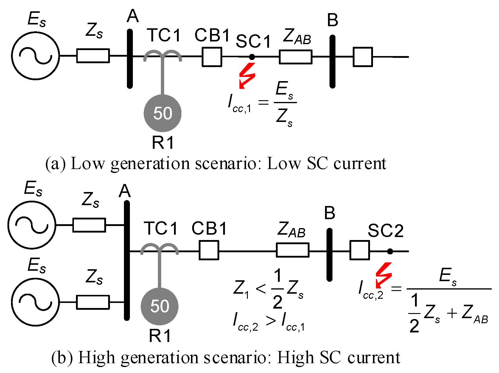
Figure 2 shows a classical situation where the setting of the IOC relay R1 for line faults is impractical (R1 setting: I_50,1 < I_cc,1 and I_50,1 > I_cc,2). In this case, the IOC relay is not suitable for OC protection because the boundary values of the short-circuit current at the relay point do not allow the fault’s discrimination.

3. Adaptive Instantaneous Overcurrent Protection: The Adjustment Algorithm

The idea of having a relay whose setting changes to adapt to the system conditions is not new; DyLiacco proposed that idea in 1967 [27]. The original idea considers the adaptive protection action as automatic but also takes into account the possibility of timely human intervention. The adaptive relay is the core of the smart adaptive protection scheme. The relay has the capability of changing its settings, characteristics, or logic functions changed online in a timely manner by means of externally generated signals or control action [5].

This paper proposed a methodology of AIOCP setting that ensures that the protection coverage remains unchanged regardless of the operating condition of the power system. A general overview of the proposed methodology is presented in Figure 3 and explained in the following sub-sections.

3.1. Positive-Sequence Phasor Estimation

The first step of the proposed methodology of AIOCP setting is the positive-sequence phasor estimation of the voltage and current at the AIOCP location. Several phasor estimation methods have been proposed in the scientific literature, including least-squares fitting (LSF) [3], discrete Fourier transform (DFT) [3,28], etc.

The process used in this paper consists of taking the sampled measurements of the waveforms of the bus voltage and of the current (v, i) and processing the signals to calculate the correspondent voltage and current phasors (V = |V|∠θ, I = |I|, taken as references to the estimation process).

The signal processing of the sampled voltages and current includes: an anti-aliasing filter, sample and hold, and an analogic/digital converter. The anti-aliasing filter is used to eliminate spectrum superposition from the sampled input voltage and current signals. Details of the analogic/digital converter are not included here.

The positive-sequence component voltage and current values are calculated using a one-cycle Fourier filter with 256 samples per cycle and a second-order Butterworth anti-aliasing analogic filter with a cut-off frequency of 360 Hz.

3.2. Identification of TEC Parameters

The core of the proposed methodology of AIOCP setting is the calculation of the TEC parameters in real time and uses the TEC to set an IOC relay adjustment criterion for the desired relay coverage. The process of identification of TEC parameters estimates in real time four electrical parameters: |E_s|, δ_s, R_s, and X_s. The algorithm described below is independent of the load model and does not require data synchronisation between the power line terminals involved in the AIOCP setting.

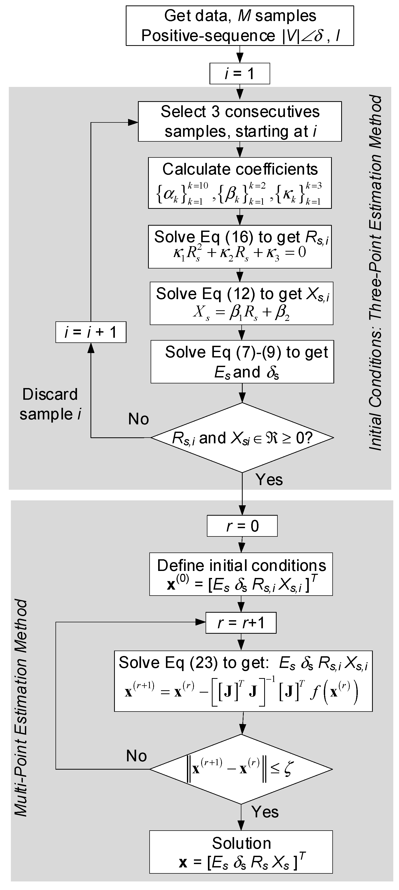
The flowchart of the real-time algorithm to identify the TEC parameters is presented in Figure 4. The algorithm’s input data are the positive-sequence voltage and current data estimated at the point of the AIOCP. Then two main processes are accomplished: (i) initial conditions are calculated based on a three-point estimation, and then (ii) a multi-point estimation method is used to calculate the TEC: |E_s|, δ_s, R_s, and X_s.

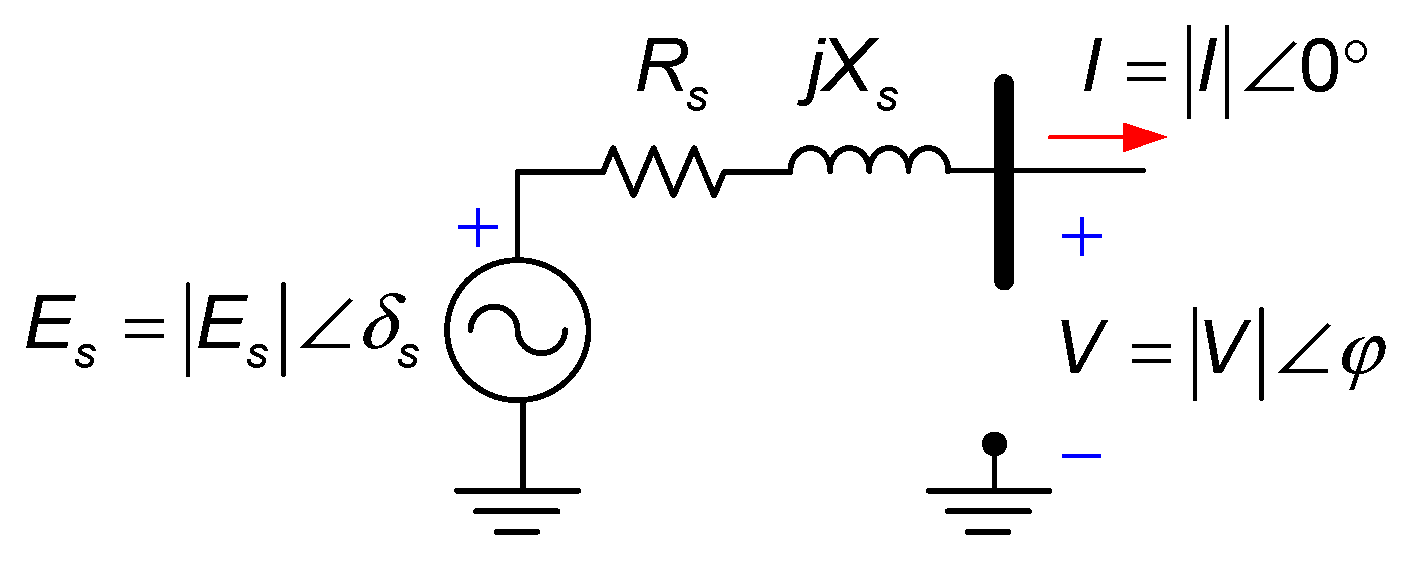
Thevenin’s theorem (TT) allows any two-port network to be reduced to a single-voltage source in series with a single impedance. Figure 5 shows the per-phase TEC for a specific three-phase node at the AIOCP location. The actual power system is assumed to be operating at a steady state, and it is symmetrical and balanced. In Figure 5, V and I represent the line-to-neutral positive-sequence voltage and current phasor (as estimated in the previous section) at the point of connection of the AIOCP. E_s represents the Thevenin’s equivalent voltage source of the system viewed from the node directly connected to the AIOCP, and Z_s is the Thevenin equivalent impedance of the node.

The loading conditions of the power system are assumed to be a constant or tiny variation in the very long term. As a consequence, the terminal conditions are represented by the positive-sequence voltage and current (V and I).

Applying the Kirchhoff voltage law (KVL) to the TEC (as shown in Figure 5) for a set of measurement data at time t_i:

$$\left(\left|E_{s,i}\right|\angle {\delta }_{s,i}\right)=\left(R_{s,i}+j{X}_{s,i}\right)\left(\left|I_i\right|\angle 0°\right)+\left(\left|V_i\right|\angle {\theta }_i\right)$$

(4)

where the subscript i represents the measurement data at time t_i. Equation (4) has seven variables. Three variables are known from the phasor estimation, |I_i|, |V_i|, and θ_i, and four variables coming from the TEC are unknown: |E_s,i|, δ_s,i, R_s,i, and X_s,i.

3.3. Initial Conditions: Three-Point Estimation Method

The method of three-point is based on the three consecutive samples of voltage and current measure at load location. The positive-sequence voltage phase, V, can be rewritten in terms of its real (V_x,i) and imaginary (V_y,i) components as:

$$V_i=V_{x,i}+j{V}_{y,i}$$

(5)

where:

$$V_{x,i}=\left|V_i\right|\cos {\theta }_i\hspace{1em}\hspace{1em}{V}_{y,i}=\left|V_i\right|\sin {\theta }_i$$

(6)

Assuming there are no changes in the internal voltage of the TEC, |E_s,i|= |E_s|, and δ_s,i = δ_s are constant in the i-th sample. The Thevenin impedance is assumed to be constant, R_s,i = R_s, and X_s,i = X_s, then (4) can be rewritten in terms of the real and imaginary component as:

$$\begin{array}{l}\left|E_s\right|\cos {\delta }_s=R_s\left|I_i\right|+V_{x,i}\\ \left|E_s\right|\sin {\delta }_s=X_s\left|I_i\right|+V_{y,i}\end{array}$$

(7)

Applying square both sides of the equation and adding them:

$${\left|E_s\right|}^2={\left(R_s\left|I_i\right|+V_{x,i}\right)}^2+{\left(X_s\left|I_i\right|+V_{y,i}\right)}^2$$

(8)

Equation (8) has three unknown variables and three known variables |I_i|, V_x,i, and V_y,i. Considering three consecutive samples (i = 1, 2, and 3):

$${\left|E_s\right|}^2={\left(R_s\left|I_1\right|+V_{x,1}\right)}^2+{\left(X_s\left|I_1\right|+V_{y,1}\right)}^2$$

(9)

$${\left|E_s\right|}^2={\left(R_s\left|I_2\right|+V_{x,2}\right)}^2+{\left(X_s\left|I_2\right|+V_{y,2}\right)}^2$$

(10)

$${\left|E_s\right|}^2={\left(R_s\left|I_3\right|+V_{x,3}\right)}^2+{\left(X_s\left|I_3\right|+V_{y,3}\right)}^2$$

(11)

The magnitude of the Thevenin voltage |E_s| is from the previous equations by equating Equations (8)–(10). The two final equations are expressed as a function of the ten coefficients (α_i, i = 1, …, 10) and two unknown variables (R_s and X_s).

$${\alpha }_1{R}_s^2+{\alpha }_2{R}_s+{\alpha }_3=-{\alpha }_1{X}_s^2+{\alpha }_4{X}_s+{\alpha }_5$$

(12)

$${\alpha }_6{R}_s^2+{\alpha }_7{R}_s+{\alpha }_8=-{\alpha }_6{X}_s^2+{\alpha }_9{X}_s+{\alpha }_{10}$$

(13)

where:

$$\begin{array}{cc}{\alpha }_1={\left|I_1\right|}^2-{\left|I_2\right|}^2\hfill & {\alpha }_2=2\left(\left|I_1\right|V_{x,1}-\left|I_2\right|V_{x,2}\right)\hfill \\ {\alpha }_3=V_{x,1}^2-V_{x,2}^2\hfill & {\alpha }_4=2\left(\left|I_2\right|V_{y,1}-\left|I_1\right|V_{y,2}\right)\hfill \\ {\alpha }_5=V_{y,2}^2-V_{y,1}^2\hfill & {\alpha }_6={\left|I_1\right|}^2-{\left|I_3\right|}^2\hfill \\ {\alpha }_7=2\left(\left|I_1\right|V_{x,1}-\left|I_3\right|V_{x,3}\right)\hfill & {\alpha }_8=V_{x,1}^2-V_{x,3}^2\hfill \\ {\alpha }_9=V_{y,3}^2-V_{y,1}^2\hfill & {\alpha }_{10}=2\left(\left|I_3\right|V_{y,3}-\left|I_1\right|V_{y,1}\right)\hfill \end{array}$$

Now, X_s is expressed as a function of R_s:

$$X_s={\beta }_1{R}_s+{\beta }_2$$

(14)

where the coefficients β₁ and β₂ are defined as:

$${\beta }_1=\frac{{\alpha }_2{\alpha }_6-{\alpha }_1{\alpha }_7}{{\alpha }_4{\alpha }_6-{\alpha }_1{\alpha }_{10}}{\beta }_2=\frac{{\alpha }_1{\alpha }_9+{\alpha }_5{\alpha }_3-{\alpha }_1{\alpha }_7-{\alpha }_5{\alpha }_6}{{\alpha }_4{\alpha }_7-{\alpha }_1{\alpha }_{10}}$$

(15)

Substituting (14) into (12):

$${\kappa }_1{R}_s^2+{\kappa }_2{R}_s+{\kappa }_3=0$$

(16)

where:

$$\begin{array}{l}{\kappa }_1={\alpha }_1\left(1+{\beta }_1^2\right)\\ {\kappa }_2={\alpha }_2+2{\alpha }_1{\beta }_1{\beta }_2-{\alpha }_4{\beta }_1\\ {\kappa }_3={\alpha }_3+{\alpha }_1{\beta }_2^2-{\alpha }_4{\beta }_2-{\alpha }_5\end{array}$$

(17)

Equation (16) represents a second-order polynomial, and the solution must be a real positive number, R_s ≥ 0. After calculating the Thevenin resistance R_s, |E_s|, and X_s can be calculated using (9)–(11) and (14). Additionally, the Thevenin inductive reactance must be a real positive (X_s ≥ 0) in order to define a feasible solution. It must be noticed the solution is highly sensitive to noise and transients in the positive-sequence voltage and current measurements. In case the solution does not satisfy the positivity condition (R_s ≥ 0 and X_s ≥ 0), the i-th measurement is discarded, the (I + 1)-th measurements are selected, and the process is repeated.

3.4. Multi-Point Estimation Method

Equation (4) can be rewritten as:

$$\left[\begin{array}{c}\left|E_s\right|\cos {\delta }_s\\ \left|E_s\right|\sin {\delta }_s\end{array}\right]=\left[\begin{array}{cc}{R}_s& 0\\ 0& X_s\end{array}\right]\left[\begin{array}{c}\left|I_i\right|\angle 0°\\ \left|I_i\right|\angle 0°\end{array}\right]+\left[\begin{array}{c}{V}_{x,i}\\ V_{y,i}\end{array}\right]$$

(18)

where the supply side of the system is assumed to be constant (|E_s| δ_s, R_s, X_s) for a set of measurements i = 1, 2, …, n.

Reordering (18):

$$\left[\begin{array}{c}\left|E_s\right|\cos {\delta }_s\\ \left|E_s\right|\sin {\delta }_s\end{array}\right]-\left[\begin{array}{cc}{R}_s& 0\\ 0& X_s\end{array}\right]\left[\begin{array}{c}\left|I_i\right|\angle 0°\\ \left|I_i\right|\angle 0°\end{array}\right]-\left[\begin{array}{c}{V}_{x,i}\\ V_{y,i}\end{array}\right]=\left[\begin{array}{c}0\\ 0\end{array}\right]$$

(19)

Equation (19) is assumed to have a residual or error (ε), the difference between the actual value of the dependent variable and the value predicted by the model.

$$\left[\begin{array}{c}\left|E_s\right|\cos {\delta }_s\\ \left|E_s\right|\sin {\delta }_s\end{array}\right]-\left[\begin{array}{cc}{R}_s& 0\\ 0& X_s\end{array}\right]\left[\begin{array}{c}\left|I_i\right|\angle 0°\\ \left|I_i\right|\angle 0°\end{array}\right]-\left[\begin{array}{c}{V}_{x,i}\\ V_{y,i}\end{array}\right]=\left[\begin{array}{c}{\epsilon }_{x,i}\\ {\epsilon }_{y,i}\end{array}\right]$$

(20)

where ε_xi and ε_xi represent the estimation errors.

Using the previous approach, the problem of estimating the parameter of the TEC is reduced to an optimisation problem (21), where the objective is to minimise the error of estimation for a number M of measurements.

$$\min \left[f\left(x\right)\right]=\min \left[{\displaystyle \sum _{i=1}^M\left({\epsilon }_i^2\right)}\right]$$

(21)

where x = [|E_s|, δ_s, R_s, X_s], and ε_i = [ε_x,i ε_y,i]^T.

The vector x minimises the function f(x), and it is an estimation of the TEC parameters and solution to the optimisation problem. The minimisation of f(x) can be obtained through iterative based methods

A set of M non-linear equations is formed: ε = [ε₁ ε₂, …, ε_M]^T, and n variables x = [|E_s|, δ_s, R_s, X_s], where M ≥ n. In this paper, Equation (21) is solved using the Gauss–Newton iterative method [2] which is a method for solving the non-linear least-squares problem. The Gauss–Newton method is based on an iterative process where the approximation of the (r + 1) iteration is calculated as:

$$x^{\left(r+1\right)}=x^{\left(r\right)}-{\left[{\left[J\right]}^{T}J\right]}^{-1}{\left[J\right]}^{T}f\left(x^{\left(r\right)}\right)$$

(22)

where x⁽⁰⁾ represents the initial condition, J is the matrix of first Jacobian derivatives, ε is the number of non-linear equations of the system (m × 1), and x is the solution to the system of equations of (n × 1). In implementing the Gauss–Newton method, the vector of variables is updated in each iteration (r). The convergence criterion is that the maximum difference of a variable between iterations must not be greater than a pre-defined threshold.

3.5. Adaptive Adjustment Algorithm

When the parameters of the TEC are known, the adaptive adjustment of the IOC protection relay (I₅₀) is calculated as.

$$I_{pickup}=I_{50}=\frac{E_s}{Z_s+XZ}$$

(23)

where E_s and Z_s are the voltage and impedance of the Thevenin equivalent estimate in real time, respectively, and XZ is the impedance of the desired coverage area. In this way, an adaptive adjustment is generated. Regardless of whether the parameters E_s and Z_s change during the normal or abnormal operation of the power system, the coverage zone (X) will remain. The general structure of the adaptive adjustment algorithm of the instantaneous overcurrent protection is presented in Figure 6.

The input of the algorithm is the desired coverage area (X) in the protected line. The algorithm includes a security verification to avoid the undesirable false trip. A counter is initialised (k = 1), which will allow the trip signal to be emitted only if the algorithm detects a fault condition. It persists during three consecutive current samples, and it increases the stability of the algorithm under transient conditions.

An initial setting of the AIOCP is defined. This setting allows the relay to trip in the case where the power line has a fault when the line is connected to the power system. The initial setting of the AIOCP (I_pickup) is calculated as traditional IOCP:

$$I_{pickup}=I_{50}=\frac{E}{Z_s+XZ}$$

(24)

where E is the nominal rms line-to-ground voltage and Z_s is the equivalent impedance behind the relay position. Afterwards, incremental current and voltage, calculated from the samples positive-sequence current and voltage [15], are used as fault detection elements. The incremental signals eliminate the steady-state components, making fault detection function immune to harmonics. A threshold (ζ) is defined in order to determine that a fault exists, which is the nominal current per secondary of the CT. If there is no fault, the condition k = 1 remains, the TEC parameters are calculated, the AIOCP setting is updated, and the algorithm continues with the next instant of time. If there is a fault, the AIOCP setting is checked. Regardless of whether the actual current is less than the AIOCP setting, the initial condition k = 1 remains, and the AIOCP setting is updated. Otherwise, as the actual current is greater than the AIOCP setting, the trip condition is checked. If k = 3, the trip command is issued, the counter k increases, the AIOCP setting remains without change, and the algorithm continues with the next instant of time. If the fault self-extinguishes before the trip condition is fulfilled (k = 3), the algorithm goes back to k = 1, and the AIOCP is updated.

The algorithm considers the following four scenarios:

• For no fault, the AIOCP setting is updated.
• For a fault outside the protection coverage area, the AIOCP setting is updated.
• During a fault, if it disappears before k = 3, the AIOCP setting is updated.
• During a fault, if it persists (k = 3), the trip command is sent to the circuit breaker.

4. Simulation Results and Discussion

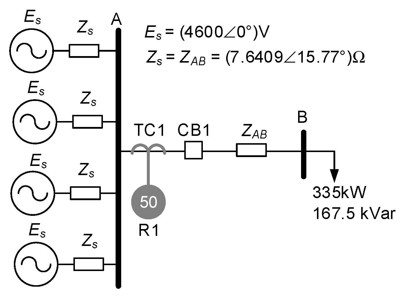
This section is dedicated to testing and demonstrating the proposed algorithm for adaptive tuning. An idealistic two-node system is used for illustrative purposes. The test system was modelled and simulated using Mathworks MATLAB. It is a three-phase, 60 Hz, balanced system. The single-phase representation is shown in Figure 7, where the sources are represented by ideal voltage sources (E_S) behind an ideal impedance (Z_s). A variable load is connected at node B (a random variation of ±5% of the loads with respect to its rated power is included). An IOC protection relay (R1) is installed to protect the power line between nodes A and B (Z_AB).

The performance of the proposed methodology of AIOCP setting is tested and demonstrated considering four different cases. Plots of the evolution of the IOC protection relay over time are used for the assessment of the performance of the adaptive protection, considering the comparison between the setting of a traditional IOC relay (I₅₀) and the adaptive one (I_50,A).

4.1. Case I: Sub-Allocation

Case I considers the four sources connected to the node (as shown in Figure 7). As a consequence, the traditional IOC relay has a fixed setting I₅₀ = 432 A, protecting 80% of the power line between nodes A and B, this situation is depicted as a continuous horizontal line at Figure 8a. The current setting of the proposed AIOC relay (I_50,A) is shown in Figure 8b, as a dashed line. Initially, the current measured by the protection corresponds to the load current, which has a value of 82 A and is represented by the dotted line (see Figure 8a). One source is disconnected from node A at 400 cycles. As a consequence, the system becomes weak as the equivalent impedance increases.

The classic IOC has its setting fixed (I₅₀ = 432 A), while the proposed AIOCP relay is able to adjust its setting to the new condition (I_50,A = 400 A). More sources are removed from the system at 800 and 1200 cycles, respectively. The adjustment of the classic IOC relay is not affected in both cases. However, the proposed AIOCP relay is still able to see the changes in the system impedances and keep protecting 80% of the line. A three-phase permanent fault at 75% of the protected line is simulated at 1400 cycles. Figure 8a shows the increase in the current measured by the protection due to the fault; however, due to the increase in the impedance, the current value does not exceed the fixed setting (|I_cc| < I₅₀), only if it exceeds the adaptive adjustment (|I_cc| > I_50,A). This means that an instantaneous overcurrent protection with a fixed setting would not detect the fault, but the proposed AIOCP setting has the appropriate sensitivity to detect the fault appropriately.

The protection coverage (%) is shown in Figure 8b. The proposed adaptive adjustment keeps coverage of 80% of the protected line constant, regardless of the system impedance change, but the classical IOC fixed setting of the coverage zone collapses at 71%, 54%, and 5%, respectively. This justifies that the fixed setting protection loses sensitivity to detect faults at 75% since it was set at 80% with a lower source impedance value.

4.2. Case II: Over-Coverage

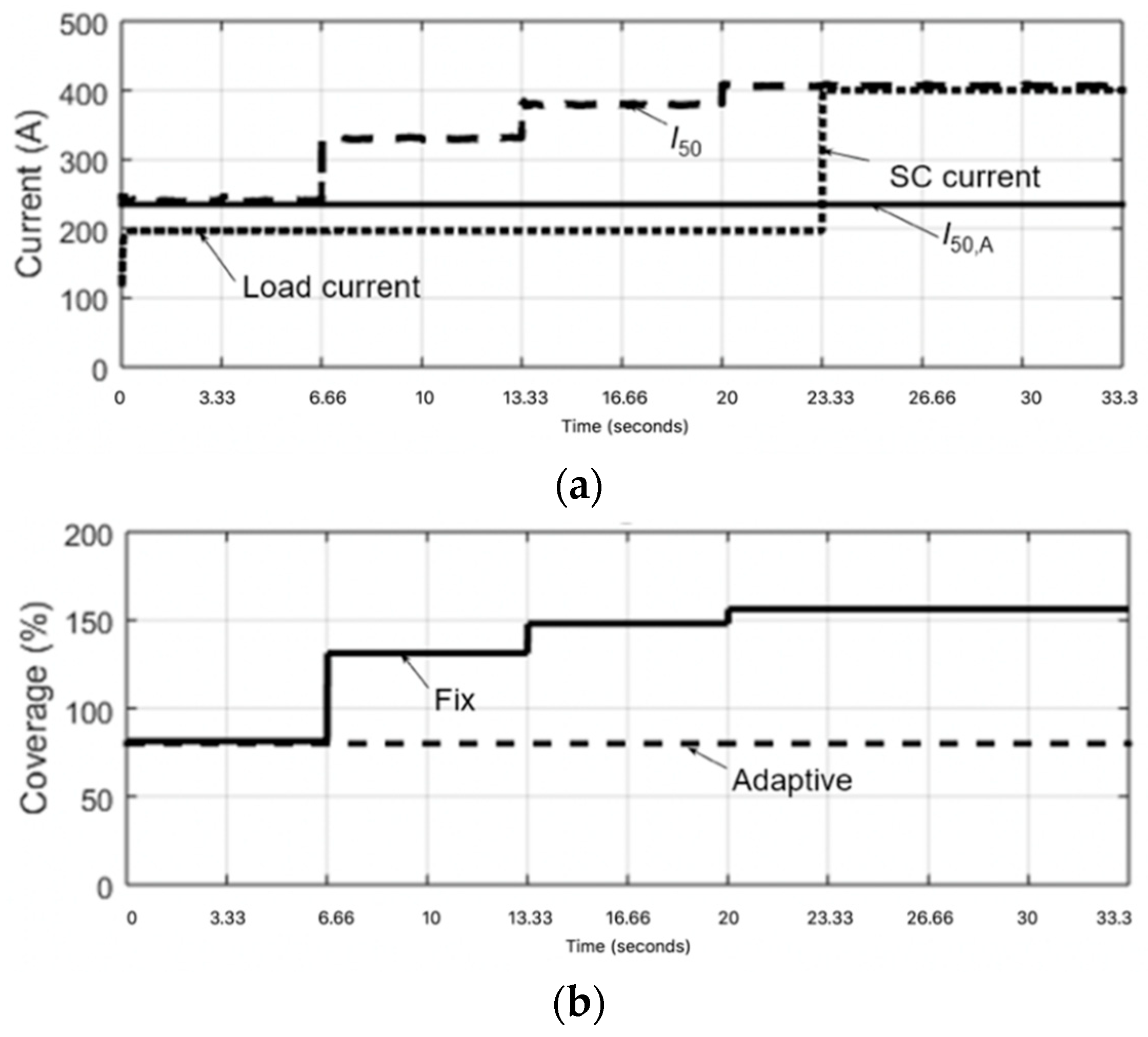
Over-coverage of an IOC relay signifies the relay’s accuracy and coordination setting because it operates at a current that is lower than the setting. Case II is designed to illustrate the problem of over-coverage. The starting point is the system shown in Figure 7 (197 A load current). Initially, a single source is connected to node A. The setting of the classical IOC relay results in I₅₀ = 235 A, protecting 80% of the line between nodes A and B. Considering the steady-state loading, the setting of the proposed AIOC relay (I_50,A) is practically the same. Figure 8a shows the IOC settings (I_50,A)

More sources are added to node A at 400, 800, and 1200 cycles. The appreciating settings of the classical and proposed AIOC relay are shown in Figure 9a. The setting of the classical IOC relay remains constant, while the adaptive relay is timely adjusted.

At 1400 cycles, a three-phase permanent fault is applied at 85% of the protected line. The classical IOCP setting could detect the fault and operate incorrectly, but the proposed AIOCP has the proper selectivity not to detect it. Figure 9b shows the protection scope of the classical IOCP (continuous line) and proposed adaptive setting (dashed line). The proposed AIOCP keeps coverage of 80% of the protected line constant, regardless of the impedance change that the network experiences.

4.3. Discussion

The analysed cases show that the proposed AIOCP is able to identify and select the appropriate setting for IOCP and keep its coverage area constant before any network condition changes occur behind the relay. It was observed how the classical IOC protection with the constant setting is affected in its coverage zones in the different scenarios analysed.

The proposed method does not require to distinguish a fault condition from the normal condition such as the load change or power loss because the Thevenin estimation is carried on with a small change in voltage and current signal due to load changes, which has a low rate of change in state-stable, and the setting values remain constants until the following update estimation. Additionally, during the transition from state-stable conditions to fault conditions, the rate of change of Thevenin impedance is very high, the proposed algorithm will not converge, and the relay setting remains unchanged.

5. Conclusions

The proposed AIOCP based on the TEC estimation can correctly identify and select the necessary IOC relay settings in real time to keep the relay coverage constant before any changes that the network may experience behind the protection. Two typical scenarios were evaluated, sub-allocation and over-coverage scenarios. The proposed algorithm correctly identified the scenario and adapted to the conditions of the system, while the fixed (traditional) adjustment was affected in its area of coverage in each change of operation of the network.