Article

Rapid Detection of Small Faults and Oscillations in Synchronous Generator Systems Using GMDH Neural Networks and High-Gain Observers

1
Department of Electrical Engineering, Azad University of Mashhad, 91735-413 Mashhad, Iran
2
Interdisciplinary Centre for Security, Reliability and Trust, University of Luxembourg, L-1855 Luxembourg, Luxembourg
3
College of Science, Health, Engineering and Education, Murdoch University, Perth, WA 6150, Australia
4
School of IT, Deakin University, Geelong, VIC 3220, Australia
5
College of Science and Engineering, Flinders University, Adelaide, SA 5042, Australia
*
Authors to whom correspondence should be addressed.
Electronics 2021, 10(21), 2637; https://doi.org/10.3390/electronics10212637
Submission received: 8 October 2021 / Revised: 23 October 2021 / Accepted: 26 October 2021 / Published: 28 October 2021
(This article belongs to the Special Issue Advances in Fault Detection/Diagnosis of Electrical Power Devices)

Abstract

:
This paper presents a robust and efficient fault detection and diagnosis framework for handling small faults and oscillations in synchronous generator (SG) systems. The proposed framework utilizes the Brunovsky form representation of nonlinear systems to mathematically formulate the fault detection problem. A differential flatness model of SG systems is provided to meet the conditions of the Brunovsky form representation. A combination of high-gain observer and group method of data handling neural network is employed to estimate the trajectory of the system and to learn/approximate the fault- and uncertainty-associated functions. The fault detection mechanism is developed based on the output residual generation and monitoring so that any unfavorable oscillation and/or fault occurrence can be detected rapidly. Accordingly, an average L1-norm criterion is proposed for rapid decision making in faulty situations. The performance of the proposed framework is investigated for two benchmark scenarios which are actuation fault and fault impact on system dynamics. The simulation results demonstrate the capacity and effectiveness of the proposed solution for rapid fault detection and diagnosis in SG systems in practice, and thus enhancing service maintenance, protection, and life cycle of SGs.

1. Introduction

Fault detection and identification (FDI) approaches for nonlinear systems have drawn attention in the last few decades, as they play a vital role in modern complex systems with a higher reliability requirement. Particularly, FDI design tackling the actuator faults is of significance. This is due to the key role of actuator effort on system stability and performance. In contrast to sensors for which the physical redundancy can be readily realized, several identical actuators are costly to be implemented as well as the increased weight, occupied space, and data acquisition complexity. On the other hand, for the large interconnected systems, e.g., wind farms [1], it is not easy to isolate the actuator faults. This stems from the different sources that cause the final malfunctions. More importantly, in the case of a small actuator fault, its symptoms may be buried in the system uncertainties or external disturbances. In such a case, the well-known approaches, such as observer design [2], parameter estimation [3], and parity space [4], fail to operate satisfactorily. It is worth noting that even though the actuator fault is small, it still may lead to degraded performance, instability, or even catastrophe.
In safety-critical systems such as synchronous generator (SG) systems, which are subject to hazardous operation conditions, even small hidden faults can result in the loss of generator, impacting the stability of the entire grid. Stator faults or ground faults in the stator windings are classified as common generator faults. The small fault currents occur specifically when the SG systems are grounded with high impedance. However, it is extremely difficult to detect such small-scale faults just by relying on differential protection functions [5]. A common solution to overcome this issue is to simultaneously use neutral overvoltage relays, percentage differential relays, and third harmonic schemes. As documented in the literature, fault detection based on the generator neutral and terminal third harmonic voltage characteristics are restricted to factors such as loading and generator design and configuration. Moreover, the proposed solution imposes an extra cost on the SG systems and additional complexity for service maintenance, protection, and real-world applications [5,6,7].
In this regard, a robust FDI system, with the capacity for fast detection of small faults, can contribute to the fault-tolerant control (FTC) module to maintain the stability and overall performance of the SG systems. In addition, the early detection of such small faults in the generator can significantly contribute to decreasing the maintenance/replacement cost and outage period. As such, different hardware-based, model-based, and data-driven approaches have been proposed in the literature [8,9,10,11,12,13,14,15,16,17,18]. A conventional class of FDI in the literature is called hardware redundancy techniques which employ multiple identical components for monitoring and acquiring data of interest and validation in a system [19,20,21]. However, the main disadvantage of this approach is imposing cost, weight, and complexity on the system. Moreover, the redundant hardware is usually used as a backup system at the occurrence of the fault and it is not able to provide any information of fault features such as fault time, fault shape, and its amplitude [10,11,20]. The second class of FDI approaches is called model-based techniques (analytical redundancy), which is established on the mathematical model of the underlying system. In this category, observer-based methods are quite popular as they can either estimate states and faults of the system directly or compare residual evaluation function with a predefined/adaptive threshold. In this regard, sliding mode observer-based FDI (SMOFDI) is a popular model-based technique that has been extensively used due to its accuracy, fast convergence, and robustness against disturbances [22,23,24,25,26,27,28]. For example, in [29,30,31], the concept of first-order SMO is utilized for actuator fault detection and in [9], the SMOFDI utilizes the principle of the equivalent injection signal to reconstruct the fault or the quantity of non-measurable system parameters. To generate a chattering-free equivalent output injunction signal, the use of low pass filters is essential; however, this imposes some delays and consequently impacts the accuracy of estimation and stability of the underlying system [32]. More recently, higher-order sliding mode observer (HSMO) techniques have been proposed to accommodate the need for low pass filters while producing chattering-free continuous estimations [33,34]. In [35], the HSMO technique for detecting a fault in a linear time-invariant system is proposed and the necessary and sufficient condition of finite time convergence is provided. However, the application of the proposed solution is restricted in practice as the information of higher-order derivatives of the sliding surface is required. In [36], an adaptive super-twisting sliding mode observer for actuator FDI is proposed. This technique enables the system to adapt and maintain a sliding motion while the system is experiencing high-frequency oscillation failures.
Finally, the third class of FDI approaches is called data-driven techniques which have been employed for fault detection and protection in SG and interconnected power systems [8,12,14,15,16,18,37]. The fundamental of these techniques is to use available sensory data for the purpose of detection and diagnosis without knowledge of physical modeling of the underlying system. As opposed to the model-based techniques, the data-driven solutions are load-dependent and require additional sensors, although their performance is not highly dependent on the accuracy of the model and parameter estimation. The main drawbacks of the data-driven solutions, however, are the limitations in rapid and accurate detection and diagnosis of different fault types and high computational training and tuning demanding, which makes their real-time implementation difficult [37,38].
To overcome the inadequacies of FDI development for SG systems discussed above, this paper develops a systematic and mathematically proven robust and efficient FDI approach with the capacity for rapid detecting and handling small faults and oscillations in practice. The FDI mechanism in this paper is developed based on output residual generation and monitoring so that any unfavorable oscillation and/or fault occurrence can be detected rapidly. To generate the residual for the FDI purpose, first, a bank of high-gain observers is constructed for both normal and faulty modes of the monitored system. A promising technology of group method of data handling neural network (GMDHNN) is utilized for the approximation of unknown dynamics and fault functions in the SG system. The rationale behind the use of GMDHNN in the proposed FDI system is to utilize a computationally efficient set of hierarchically connected networks rather than a complex neural model for uncertainty and system fault approximation which accommodates the difficulties of rapid fault detection in practice. Finally, an average L1-norm criterion is proposed for rapid decision making in faulty situations. In summary, this paper provides the following contributions:
-
A systematic FDI procedure with the capacity of rapid detection of small faults and oscillations in the SG system is presented.
-
A differential flatness approach is employed to model the SG system in a Brunovsky form utilizable for the FDI procedure.
-
A bank of a practically implementable high-gain observer is developed for state estimation of the SG system in both healthy and faulty mode.
-
A computationally efficient and real-time implementable GMDHNN is developed to approximate unknown dynamics and fault functions in the SG system.
-
A decision-making mechanism for the detection of small oscillation and fault occurrence based on an average L1-norm criterion is proposed.
The rest of the paper is organized as follows. In Section 2, technical preliminaries and problem statements are presented. In Section 3, first, the original third-order model of SG is presented and then the flatness-based representation is developed to meet the condition of Brunovsky form systems described in Section 1. In Section 4, the GMDHNN-based FDI design procedure including the essence of GMDHNN, high-gain observer design, and FDI decision-making mechanism is discussed in detail. Section 5 demonstrates simulation results and performance evaluation of the proposed FDI system for two benchmark scenarios of actuation fault and fault impact on the system’s dynamics. Finally, Section 6, presents the conclusion of this paper.

2. Technical Preliminaries and Problem Description

2.1. Technical Preliminaries

Let us consider the strict feedback nonlinear system in a Brunovsky form including faults and disturbances as (1):
{ x ˙ 1 = x 2 x ˙ 2 = x 3         .         .         . x ˙ n 1 = x n x ˙ n = f ( x , x ˙ , , x ( n 1 ) ) + g ( x , x ˙ , , x ( n 1 ) ) u + η ( t T 0 ) Λ φ ( x , u ) + d ( t ) y = x 1
where x i , i = 1 , , n , is the unknown states vector, u represents the control input vector, y is the output, f ( . ) is the continuous nonlinear function of the system dynamics, g ( . ) represents the continuous nonlinear mapping function associated with the input, and Λ φ ( . ) represents the impact of the fault φ on the system dynamics. Indeed, the variation of Λ φ ( . ) deteriorates the actuator effort g ( . ) u . On the other hand, η ( t T 0 ) is the fault time profile including the unknown fault time occurrence of T 0 , such that for t < T 0 , η ( t T 0 ) = 0 , otherwise, η ( t T 0 ) = 1 . d ( t ) represents unknown bounded disturbances.
To initiate the design, the following assumptions are made in the design procedure.
Assumption 1.
The system states and controls are always bounded even under faults; that is, ( x , u )   Ω     n + 1 ,   t t 0 where Ω is a compact set. It is assumed that the disturbance is bounded, i.e., | d ( t ) | < d ¯ , where d ¯ > 0 and d ¯ is known constant.
Assumption 2.
The continuous nonlinear functions f ( . ) and g ( . ) can be expressed as a combination of a nominal part and an unknown part, that is:
f ( x , x ˙ ,   , x ( n 1 ) ) = f o ( x , x ˙ ,   , x ( n 1 ) ) + υ ( x , x ˙ ,   , x ( n 1 ) )
g ( x , x ˙ ,   , x ( n 1 ) ) = g o ( x , x ˙ ,   , x ( n 1 ) ) + σ ( x , x ˙ ,   , x ( n 1 ) )
where f o ( . )   and g o ( . ) are the nominal parts of f ( . ) and g ( . ) , respectively, and υ ( . ) and σ ( . ) represent unknown continuous bounded uncertainties associated with f ( . ) and g ( . ) , respectively.
Assumption 3.
The system trajectories in normal and fault modes are presented as ϕ 0 ( x ( t < T 0 ) , u ( t < T 0 ) ) and ϕ s ( x ( t T 0 ) , u ( t T 0 ) ) , respectively, and are in oscillations.
Assumption 4.
The nonlinear terms f o ( . ) , g o ( . ) , υ ( . ) , σ ( . ) , and Λ φ ( . ) are local Lipchitz around x , i.e.,
| f o ( x , x ˙ ,   , x ( n 1 ) ) f o ( x ^ , x ^ ˙ ,   , x ^ ( n 1 ) ) |   ρ 1 | x x ^ |
| g o ( x , x ˙ ,   , x ( n 1 ) ) g o ( x ^ , x ^ ˙ ,   , x ^ ( n 1 ) ) |   ρ 2 | x x ^ |
| υ ( x , x ˙ ,   , x ( n 1 ) ) υ ( x ^ , x ^ ˙ ,   , x ^ ( n 1 ) ) |   ρ 3 | x x ^ |
| σ ( x , x ˙ ,   , x ( n 1 ) ) σ ( x ^ , x ^ ˙ ,   , x ^ ( n 1 ) ) |   ρ 4 | x x ^ |
| Λ φ ( x , u ) Λ φ ( x ^ , u ) |   ρ 5 | x x ^ |
where ρ i   ( i = 1 , . , 5 ) represents local Lipchitz constants in the set X , where X is the system operation set, i.e.,   x ,   x ^   X ,   u   U , and U is an admissible control set.
Assumption 5.
The fault magnitude ratio factor is bounded and defined as:
0 < 𝓅 = | Λ φ ( x , u ) | β ¯ < 1
where β ¯ is the upper bound of the modeling uncertainty β = υ ( . ) + σ ( . ) + d ( t ) , i.e., | υ ( . ) + σ ( . ) + d ( t ) | β ¯ .
Remark 1.
Assumptions 1 and 4 consider the reasonable aspects of the practical dynamic systems, i.e., the unbounded signals and their variation are not admissible. Assumption 2 considers the system uncertainties, covering a variety of model mismatches and variations. Assumption 5 stands for the small faults, i.e., the fault size is smaller than the upper bound of model uncertainties and disturbance. In such a case, the system state variation due to the fault may be buried under the effects of model uncertainties and disturbance. Therefore, most developed FDI schemes fail to detect the fault accurately [39,40,41].

2.2. Problem Description

The main objective of this paper is to develop a rapid FDI system for the SG model to be used in real time and in practice. In order to develop a rapid fault detection system for the SG model, enabling the detection of even small-magnitude faults, the following requirements should be addressed:
(1)
The dynamic model of SG should be in a Brunovsky form, as described in system (1).
Remark 2.
The Brunovsky representation of a system is a popular controllable canonical form including a finite set of integrators which allows implementing the strict state feedback and linear observers. Thus, the differential flatness property of the system is utilized to transform the original model of the generator into the Brunovsky representation.
(2)
The SG states in the nominal form should be estimated robustly.
Remark 3.
In practice, the measurement of all system states is often not available. On the other hand, information on states’ trajectories of SG is essential for persistent monitoring and diagnosis of any small oscillation/fault in the system. The nominal states’ trajectories can be estimated robustly via a linear high-gain observer due to the representation of the system in the Brunovsky form. This is incorporated in the neural network module.
(3)
The unknown dynamics in (2) and (3) should be approximated accurately.
Remark 4.
There exist unknown dynamics and uncertainties associated with the model of generators in practice. These unmodeled dynamics should be approximated to enable the design of FDI. To solve this problem, a rigorous function approximator method with the capacity of learning and approximating unknown dynamics in a local region along any arbitrary recurrent or periodic trajectory should be employed. This results in the exponential stability of the system (1) and is achieved via GMDHNN.
(4)
A bank of dynamical estimators should be developed to produce fault residual and consequently detect the real-time fault occurrence at T 0 .
Remark 5.
The dynamical estimators take advantage of the learned knowledge of the system and are established upon a bank of non-high gain observers to produce necessary information for the residual generation and decision making on the fault occurrence at T 0 .
In the subsequent sections of this paper, we show how to address the mentioned requirements.

3. The SG Model

3.1. Third Order SG Model

The connection of an SG to a power grid is illustrated in Figure 1. This configuration is known as a single-machine infinite bus (SMIB) model. In this model, the generator is connected to the rest of the network via a transformer and purely reactive transmission lines. The infinite bus is the representation of a machine that rotates at a synchronous speed of ω o and has the capacity to absorb or deliver any energy amount. The classic third-order dynamical model of this configuration in Figure 1 includes mechanical and electrical dynamic models of SG [42,43]. The mechanical dynamics of SG are as follows:
δ ˙ = ω ω 0
ω ˙ = D 2 J   ( ω ω 0 ) + ω 0 2 J ( P m P e )
where δ is power angle of the generator, ω is rotor speed with respect to the synchronous reference, ω 0 represents the synchronous speed of the generator, J is the generator’s moment of inertia, P m is the mechanical input torque to the generator, D is the damping constant of the generator, and P e is the electrical torque corresponding to the active power of the generator. The electrical dynamical model of SG is as follows:
  E ´ ˙ q =   1 T d 0   ( E f E q )
where   E ´ q is the quadrature-axis transient voltage of the generator,   E q is the quadrature-axis voltage of the generator, E f is the equivalent voltage in the excitation coil, and T d 0 represents the direct-axis open-circuit transient time constant of the generator.
The algebraic equations of the SG are given in (13).
{ E q = x d Σ x ´ d Σ   E q ´ ( x d x ´ d ) I d I d = E q ´ x ´ d Σ V s x ´ d Σ cos ( δ ) I q = V s x ´ d Σ sin ( δ ) P e = E q ´ V s x ´ d Σ sin ( δ ) Q e = E q ´ V s x d Σ cos ( δ ) V s 2 x d Σ V t = ( E q ´ x ´ d I d ) 2 + ( x ´ d I q ) 2
where x d Σ = x d + x T + x L , x ´ d Σ = x ´ d + x T + x L ; x d represents the direct-axis synchronous reactance; x ´ d is the direct-axis transient reactance; x T represents the reactance of the transformer; x L is the reactance of the transmission line; I d and I q are direct and quadrature axis currents of generator, respectively; V s represents the infinite bus voltage; Q e is the generator reactive power that is delivered to the infinite bus; and V t represents the terminal voltage of the generator.
Now, let us substitute Equation (13) into the mechanical and electrical dynamic equations of the SG in (10)–(12). This results in the complete model of SMIB systems as presented in (14)–(16):
δ ˙ = ω ω 0
ω ˙ = D 2 J ( ω ω 0 ) + ω 0 P m 2 J ω 0 2 J V s E ´ q x ´ d Σ s i n ( δ )
E ´ ˙ q = 1 T ´ d E ´ q + 1 T d 0 x d x ´ d x ´ d Σ V s c o s ( δ ) + 1 T d 0   E f
where T d ´ = x ´ d Σ x d Σ   T d 0 represents the time constant of the field winding. The SMIB model indicated in (14)–(16) can be further expressed by the general nonlinear state–space representation of the form (17):
x ˙ = f ( x ) + g ( x ) u
where x = [ δ   ω   E ´ q ] T is the state vector, and f ( x ) and g ( x ) are as follows:
f ( x ) = ( ω ω 0 D 2 J ( ω ω 0 ) + ω 0 P m 2 J ω 0 2 J V s E ´ q x ´ d Σ s i n ( δ ) 1 T ´ d E ´ q + 1 T d 0 x d x ´ d x ´ d Σ V s c o s ( δ ) ) ,   g ( x ) = ( 0 , 0 , 1 T d 0 ) T
The control input and the measurable output are defined as u = E f and y = δ , respectively. Evidently, the SG model (18) does not satisfy the Brunovsky form requirement. This issue is resolved by using the differential flatness concept.

3.2. Flatness-Based SG Model

In order to meet the system requirement of the Brunovsky form in system (1), the differential flatness theory is employed [44] and then, a flatness-based model of SG is developed.
Definition 1.
Suppose system (1) excludes the fault function and disturbance. The proposed system, which is briefly expressed by x ˙ = f ( . ) + g ( . ) u , is called differentially flat if there exists an output vector 𝓏 m in conjunction with mapping functions 𝒽 : n × ( m ) r + 1 m , ϕ : ( m ) r n , and ψ : ( m ) r + 1 m such that 𝓏 = ( 𝓏 1 ,   , 𝓏 m ) = 𝒽 ( x , u , u ˙ , ,   u ( r ) ) implies the following expressions:
{ x = ϕ ( 𝓏 , 𝓏 ˙ ,   ,   𝓏 ( r 1 ) ) u = ψ ( 𝓏 , 𝓏 ˙ ,   ,   𝓏 ( r ) )      
Definition 1 demonstrates that all the system states and controls can be expressed in terms of the flat output and a finite number of its derivatives. As a result, the differential flatness theory can be used as a useful tool to transform the general nonlinear representation of a flat system into a controllable Brunovsky form facilitating the observer and feedback control design. Next, we investigate the flatness-based model of SG.
Let us define the flat output as z = x 1 . Then, all state variables and its control inputs of the model (14)–(16) can be written as functions of the flat output and its derivatives as follows:
{ x 1 = z                                                                   x 2 = z ˙                                                                   x 3 = ω 0 P m 2 J z ¨ D z ˙ 2 J ω 0 V s 2 J x ´ d Σ s i n ( z )                          
where
z ¨ = D 2 J z ˙ + ω 0 P m 2 J ω 0 2 J V s x 3 x ´ d Σ s i n ( z )  
for z n π ,   n = 0 , 1 , 2 , . Similarly, the control input can be written as:
u = T d 0 ( x 3 ˙ + 1 T ´ d x 3 1 T d 0 x d x ´ d x ´ d Σ V s c o s ( z ) )
Equations (20)–(22) hold the differential flatness property of the SG model. Now, let us apply the variable changes as z 1 = z ,   z 2 = z ˙ ,   z 3 = z ¨ . Then, the SG model can be written in the following Brunovsky from:
[ z ˙ 1 z ˙ 2 z ˙ 3 ] = [ 0 0 0   1 0 0   0 1 0 ] [ z 1 z 2 z 3 ] + [ 0 0 1 ] v
where v is the control input for the system (23) defined as:
v = f b ( z ,   z ˙ ,   z ¨ ¨ ) + g b ( z ,   z ˙ ,   z ¨ ¨ ) u = ( ( D 2 J 2 ) z ˙ ω 0 D 2 J P m 2 J + ω 0 D ( 2 J ) 2 V s x d Σ x 3 s i n ( z ˙ ) + ω 0 2 J V s x ´ d Σ 1 T ´ d x 3 s i n ( z ) ω 0 2 J V s x ´ d Σ 1 T d 0 x d x ´ d x ´ d Σ V s   cos ( z ) s i n ( z ) ω 0 2 J V s x d Σ x 3 c o s ( z ) z ˙ ) + ( ω 0 2 J 1 T d 0 V s x d Σ s i n ( z ) ) u
Equation (24) provides the flatness-based model of SG and hence meets the requirements of system (1).

4. FDI Design Process

In this section, the FDI mechanism is established based on the GMDHNN and high-gain observer, utilized for the approximation of unknown dynamics, system states, and fault function in system (1). To this end, first, the essence of GMDHNN is briefly presented, followed by the role of the high-gain observer that provides estimates of states as a regressor vector for the proposed GMDHNN. Finally, the residual generation and FDI algorithms are presented.

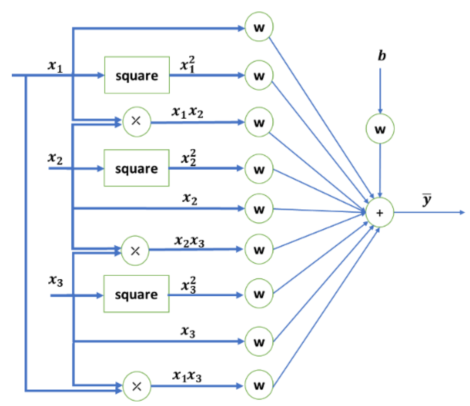
4.1. The Essence of GMDH Neural Network

The GMDHNN can be employed for nonlinear function approximation and provides more flexibility in design and robustness in performance over the conventional neural networks, such as multi-layer perceptron [45,46]. The rationale behind the GMDHNN is to utilize a set of hierarchically connected networks rather than a complex neural model for function approximation and system identification purposes. Automatic selection of a network structure just based on the measured data becomes possible in GMDHNN and thus, modeling uncertainty, as a result of neural networks structure, is accommodated to a great extent. The GMDHNN is a layered structure network in which each layer consists of pairs of independent neurons being linked via a quadratic polynomial. In all layers, new neurons are developed on the connections of the previous layers. In this self-organized neural structure, the input–output relationship is obtained via the Kolmogorov–Gabor polynomial of the form [47,48,49]:
y ¯ = a 0 + i = 1 n a i x i + i = 1 n j = 1 n a i j x i x j + i = 1 n j = 1 n k = 1 n a i j k x i x j x k +
where y ¯ represents the network’s output, the input vector is represented by X = (x1, x2, x3,…, xn), (   a i , a i j , a i j k ) represents the coefficient of the quadratic polynomial, and i, j, k  (1, 2,…, n).
To implement a GMDHNN, the following steps can be adopted:
-
Step 1: Neurons with inputs consist of all possible couple of input variables that are ( n 2 ) are developed.
-
Step 2: The neurons with higher error rates are ignored and other neurons are utilized to construct the next layer. In this regard, each neuron is used to calculate the quadratic polynomial.
-
Step 3: The second layer is constructed via the output of the first layer and hence, a higher-order polynomial is developed. Then, Step 2 is repeated to determine the optimal output utilized for the next layer input. This process is continued until the termination condition is fulfilled, i.e., the function approximation is achieved with the desired accuracy.
The above procedure indicates the evolution of the GMDHNN structure by which more desired quality of system approximation and identification can be obtained. This approach addresses the weakness of classic neural networks in system identification, as the determination of appropriate structures (including hidden layers and number of neurons) is often a cumbersome and tedious process.
To employ a GMDHHNN for FDI purposes, let us define the network by:
f n n ( k , W ) = ( W 1 ( 1 ) , ,   W n 1 ( 1 ) , ,   W 1 ( l ) , ,   W n l ( l ) )
where ( . ) represents the GMDHNN structure, l denotes the number of layers in the GMDHNN, and n l expresses the number of neurons in the l t h layer. In the proposed network (26), each neuron’s model is as:
f n ( l ) ( k , W n ( l ) ) = ξ ( ( ψ n l ( k ) ) T W n ( l ) )
where f n ( l ) ( k ) represents the output of the nth neuron in the lth layer based on the kth input signal, ξ ( . ) expresses the nonlinear invertible activation function, ψ n l ( k ) are the regressor vectors, and W n ( l ) represent the parameter vectors.
Remark 6.
Proven in [49], for any function f ( k ) : Ω k where Ω k q is a compact set, there exists an ideal parameter (weight) vector W * that satisfies the following equation:
Θ = { W * n p | f ( k ) ε ¯ ( k ) ψ ( k ) T W * f ( k ) ε _ ( k ) ,   k = 1 , , n T }  
where ε ( k ) [   ε _ ( k ) ,   ε ¯ ( k )   ] represents the bounded approximation error.
There exists a spectrum of GMDHNN algorithms in the state-of-the-art for obtaining an ideal weight vector [49,50]; in this study, the following theorem is used for updating the weight vector.
Theorem 1.
Let us consider the following dynamical GMDHNN for the approximation of a dynamic f(x) in an nth-order controllable canonical system x ˙ n = f ( x ) :
χ ˙ = α ( χ x ^ n ) + ψ ( x ^ ) T W
where χ represents the state of dynamical GMDHNN, x ^ n is an estimated state variable obtained by any observer, α is the design constant, and ψ ( x ^ ) T W denotes a GMDHNN used for approximation of f(x). The adaptation law for the weight vector W is provided by (30):
W ˙ = Γ ψ ( x ^ ) T x ¯ n Γ μ W
where Γ = Γ T > 0 is the learning coefficient, μ > 0 is a small value, and x ¯ n is defined as x ¯ n : =   χ x ^ n .
For the sake of brevity, the proof of Theorem 1 is not presented here and can be found in [51].

4.2. High-Gain Observer Design

In the past three decades, the design and development of high-gain observers have been under the attention of nonlinear system control communities to be used for output feedback control of nonlinear systems [52]. The main idea behind the high-gain observers is to separate a nonlinear system into linear and nonlinear parts and obtain the gain of the observer in such a way that the linear part becomes dominant over the nonlinear part [52,53]. This is carried out by selecting the observer gains large enough to converge the observation error into a sufficiently small region in a finite time, i.e., a neighborhood of the system state trajectory.
In order to implement the FDI mechanism, the estimate of full states of system (1) (or, equivalently, (23)) is required. To this end, a high-gain observer, which only uses the output information, is designed in the following theorem.
Theorem 2.
Consider system (1) in conjunction with Assumptions 1–5. The following high-gain observer is designed to estimate the system states, i.e., the estimation error asymptotically converges to a sufficiently small neighborhood of the origin.
{ x ^ ˙ 1   = x ^ 2   + α 1 κ   ( y y ^ )   x ^ ˙ 2   = x ^ 3   + α 2 κ 2 ( y y ^ )         .         .         . x ^ ˙ n 1   = x ^ n   + α n 1 κ n 1   ( y y ^ ) x ^ ˙ n   = f o ( x ^ , x ^ ˙ ,   , x ^ ( n 1 ) ) + g o ( x ^ , x ^ ˙ ,   , x ^ ( n 1 ) )   u + α n κ n ( y y ^ ) y ^ = x ^ 1  
where α i ( i = 1 , , n )   and κ are constant values and α i should be chosen in a way to make s n + α 1 s n 1 + + α n 1 s + α n Hurwitz polynomial with distinct roots; x ^ i   is the estimate of the system states x i ; and y ^ represents the system’s output estimate.
For the sake of brevity, the proof of Theorem 2 is not presented here, as it is similar to the proof of [51,54].
Remark 7.
Theorem 2 indicates that the observer (31) only requires the output y ( t ) to estimate the states of the system. To achieve the convergence of the estimates x ^ i   to a sufficiently small neighborhood of the system states, and hence to reduce the estimation errors, κ should be chosen large enough.
It should be noted that known functions associated with f ( . ) and g ( . ) in system (1) depend on the system states of (1). Therefore, x ^ i   can be used instead of the x i as the input to the GMDHNN to approximate f ( . ) and g ( . ) when x i   x ^ i   , i.e.,
{ f ^ ( x i | w f ) = S f ( x i ^ ) T w f + ϵ i ( x i ^ ) g ^ ( x i | w g ) = S g ( x i ^ ) T w g + ϵ i ( x i ^ )
where f ^ ( x i | w f ) and g ^ ( x i | w g ) represent approximations of f ( . ) and g ( . ) , respectively; S f ( x i ^ ) and S g ( x i ^ ) are basis functions associated with f ( . ) and g ( . ) , respectively, in the GMDHNN; and ϵ i ( x i ^ ) ϵ is an approximation error. w f and w g are ideal weight vectors on the compact sets Ω f w and Ω g w associated with f ( . ) and g ( . ) , respectively, which minimize ϵ i ( x i ^ ) when x i   x ^ i   , i.e.,
{ w f = arg min w f Ω f w [ sup x Ω x |   f ^ ( x i | w f ) f ( . ) |   ]                         w g = arg min w g Ω g w [ sup x Ω x |   g ^ ( x i | w f ) g ( . ) |   ]                        

4.3. FDI Mechanism

The FDI mechanism in this paper is developed based on output residual generation and monitoring so that any unfavorable oscillation and/or fault occurrence can be detected rapidly. To generate the residual for the FDI purpose, first, the following bank of N+1 observers are constructed for both normal and faulty modes of the monitored system (1):
{ x ^ ˙ 1 s = x ^ 2 s   + κ 1   ( y y ^ s ) x ^ ˙ 2 s = x ^ 3 s + κ 2 ( y y ^ s )           .         .         . x ^ ˙ n 1 s = x ^ n s + κ n 1   ( y y ^ s ) x ^ ˙ n s = f 0 ( x ^ s , x ^ ˙ s ,   , x ^ s ( n 1 ) ) + g 0 ( x ^ s , x ^ ˙ s ,   , x ^ s ( n 1 ) ) u + W f ¯ s T S f ( x ^ s ) + W g ¯ s T S g ( x ^ s ) + κ n   ( y y ^ s ) y ^ s = x ^ 1 s        
where x ^ s   n represents the state vector of the estimator, y ^ s represents the estimated output, and s = { 0 , 1 , , N } indicates the sth estimator. W f ¯ s T S f ( x ^ s ) and W g ¯ s T S g ( x ^ s ) compose the GMDHNN for the approximation of the unknown dynamics and fault functions. Κ = [ κ 1 , , κ n ] T   represents the observer gains, which are identical for all normal and fault estimators.
Theorem 3.
The residual y ˜ s = y y ^ s will asymptotically converge to a small neighborhood of origin if the estimator gain Κ in (34) is chosen so that the residual dynamic matrix A ¯ = ( A Κ C T ) , obtained by comparing (1) and (34), is stable and for all eigenvalues of A and all the eigenvalues of A ¯ satisfy:
R e ( λ ) > Κ 2 ( P ) ρ s ,       s = 0 , 1 , , N
where A ¯ = P Λ P 1 , P is a symmetric positive definite matrix, Κ 2 ( P ) is the condition number of matrix P, and ρ s is defined as follows:
{ ρ s = i = 1 4 ρ i   ,     f o r   s = 0                                   ρ s = i = 1 5 ρ i   ,     f o r   s = 1 , 2 , , N  
where ρ i represents the Lipchitz constants defined in (4)–(8).
For the sake of brevity, the proof of Theorem 3 is not presented here, as it is similar to the proof of [51].
The result of Theorem 3 enables us to utilize the average L1-norm for the FDI mechanism as follows:
y ˜ s ( t ) 1 = 1 T   t T t   | y ˜ s ( τ ) d τ | ,       t T
where T is a design parameter and represents the time window length of the residual. It should be noted that the robustness and rapidness of the FDI mechanism are functions of the time window length, as the larger T increases the robustness of the FDI mechanism by making the residual norm (37) less sensitive to noise but decreases the rapidness as the system should be monitored under a longer residual window time. Hence, the designer deals with a compromise in tuning T. Accordingly, by considering (37) and the following lemma, the fault detection decision is made.
Lemma 1.
The decision on the occurrence of a fault on the system (1) is made if there exists some finite time, as T d , and for some s { 1 , 2 , , N } , such that y ˜ s ( T d ) 1 < y ˜ 0 ( T d ) 1 . This yields the fault detection time t d = T d T 0 [54].
For the sake of summarization, we exclude the analysis of the fault detectability in this paper; interested readers can refer to [54].
Consequently, Algorithm 1 summarizes the FDI mechanism of this paper.
Algorithm 1 FDI Mechanism
High-gain Observer
Construct the high-gain observer (31) to estimate the states ( x ^ i   ) and output ( y ^ ) of the system (1).
GMDHNN
Construct a GMDHNN using (26) and (27);
Use the estimated states ( x ^ i   ) in (31) as a regressor vector in the GMDHNN.
Employ the adaptation law (30) for training the network and obtaining the ideal weight vector.
Use the developed GMDHNN for the approximation of unmodeled dynamics in (2) and (3) and fault function Λ φ ( x , u ) .
Residual Generation
Construct the bank of N+1 observer (34) for both healthy and faulty modes of the system.
Develop the L1-norm residual (37) to constantly monitor the system status.
Decision Making
Use Lemma 1 for decision making on the fault occurrence and determining the fault detection time t d = T d T 0 .

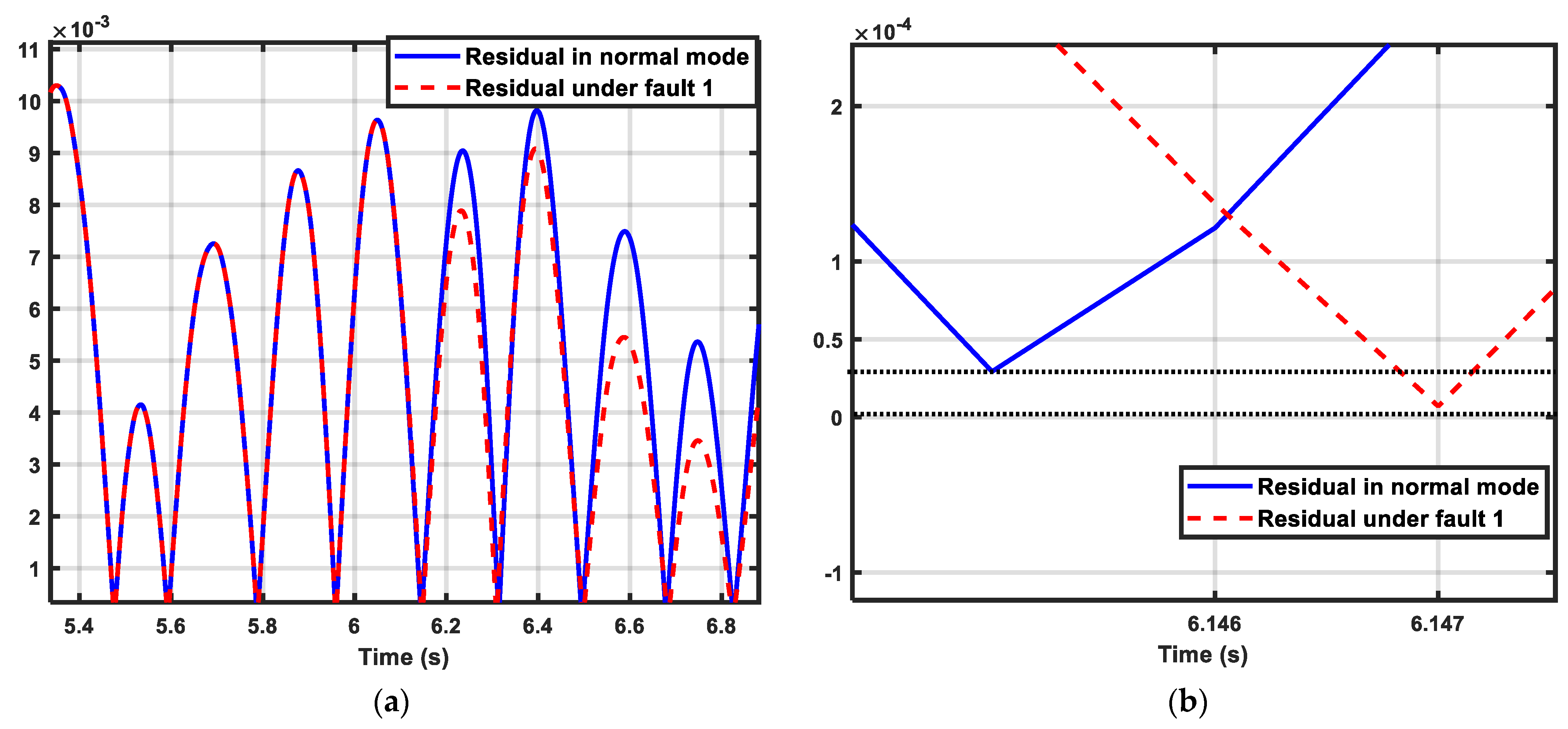
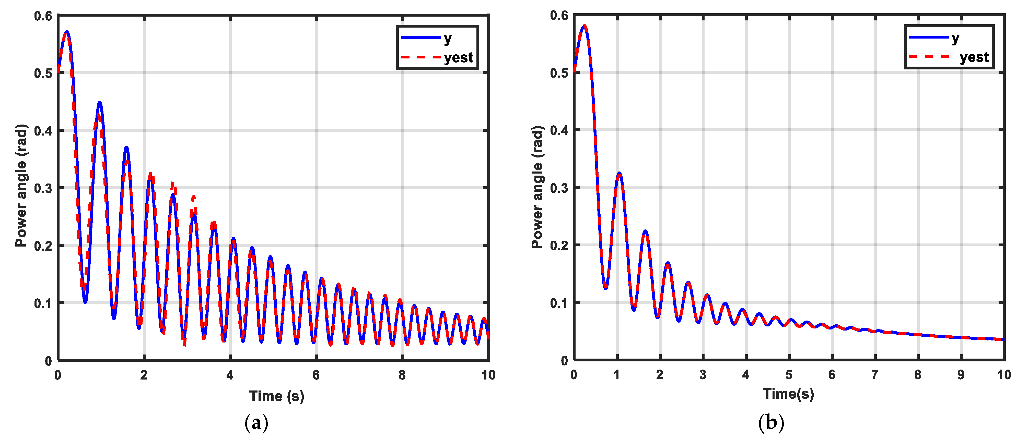
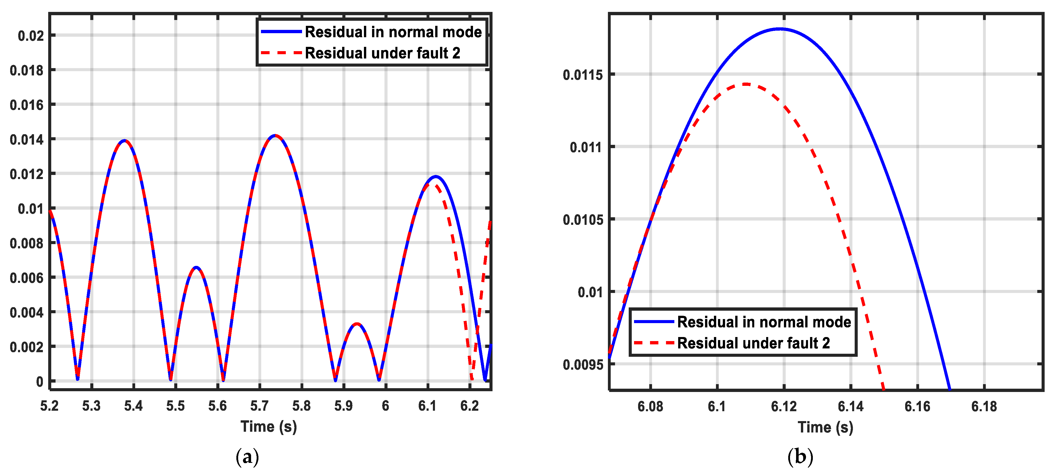
5. Results and Discussion

In this section, the effectiveness and robustness of the proposed fault detection system are demonstrated through extensive simulation studies. In this study, all computations were performed on a desktop PC with an Intel i7 3.20-GHz quad-core processor in MATLAB 2021a. The SG system (23) is simulated based on the parameters tabulated in Table 1 [42,43]. The SG is excited by u = 2 s i n ( 2 π t ) c o s ( t ) and unknown disturbance d ( t ) = 0.01 s i n ( t ) + 0.02 c o s ( 0.5 t ) is imposed on the system. The GMDHNN uses topology as illustrated in Figure 2 and for the training phase, its weighting vector W is initialized by zero. The weights are updated according to (29) and (30), and the design parameters are chosen as α = 1 , Γ = 1.5 , μ = 0.05 . Similarly, in the training phase, the design parameters for the high-gain observer (31) are set as α 1 = 4, α 2 = 8 , α 3 = 12 , κ = 5 .
Two scenarios are defined for the performance assessment of the proposed FDI system. In the first scenario, the SG is experiencing an actuation fault defined as u = u ¯ + ( q u 1 ) u ¯ where u ¯ is the control signal in the healthy mode and q u   = 0.1, which means 10% fault on the actuator. In the second scenario, a fault model impacting the system dynamics of the SG, Λ φ ( x , u ) = x 3 , is considered. This is a general purpose scenario and for example, the short-circuit fault can be categorized under scenario 2 by just considering the infinite bus voltage V s = 0 [55,56].
Figure 3 compares the SG’s state trajectories in normal and fault modes. Figure 4 focuses on the comparison of fault functions and modeling uncertainty involved with the SG. This confirms that magnitudes of both fault functions are smaller than the SG’s modeling uncertainty, a sort of indication of the difficulty of detecting such small magnitude faults in practice (as described in Section 1). Figure 5 represents the estimation of the system’s output under actuator and system dynamics faults. This confirms the fidelity and high accuracy of both trained GMDHNN and the high-gain observer for the diagnosis phase of the fault detection process.
To evaluate the performance of the FDI system in the diagnosis phase, a bank of four nonlinear observers (34) incorporating the knowledge of the trained GMDHNN, is constructed. In this regard, the observer gains are defined as κ 1 = 4 , κ 12 = 8 , κ 3 = 12 .
In the first scenario, the actuation fault on the SG model is applied at T0 = 6 s. The L1-norm residual (37) with a length of the time interval T = 20 is utilized for constantly monitoring the system status. Figure 6 illustrates the profile of the L1-norm residual for both normal and fault modes. This figure obeys Lemma 1 and thus, the detection of the fault as the residual of actuation fault becomes smaller than the normal one at the time of the fault detection, Td = 6.147 s.
Similarly, in the second scenario, the corresponding fault is applied on the SG model at T0 = 6 s. Figure 7 shows the profile of the L1-norm residual of this scenario and confirms that at the time of the fault detection, Td = 6.089 s, the average L1-norm of the fault becomes smaller than the normal counterpart, thus obeying Lemma 1 and the detection of the fault very rapidly, td = 0.1 s.

6. Conclusions

This paper developed an FDI framework to rapidly detect the small faults and oscillations in SG systems. The proposed framework was established upon the GMDHNN and high-gain observer to estimate the trajectory of the system and to approximate uncertainties associated with unmodeled dynamics and external disturbances in the SG. The fault detection mechanism was developed based on the average L1-norm criterion for rapid decision making in faulty situations. The performance of the proposed framework was investigated via simulation studies. In this regard, two benchmark scenarios of the actuation fault and fault impact on system dynamic changes were applied on the SG. The simulation results confirmed the fidelity, effectiveness, and robustness of the proposed FDI system in fast detection of small-magnitude faults on the SG system, which is promising for practical applications. An example of these practical applications includes fast fault detection in the critical truncation systems in electric vehicles, electric trains, etc. The future line of this research will focus on integrating the proposed FDI system with a robust FTC module based on sliding mode control [57,58,59,60] and include the impact of sensor faults, as well. Moreover, the performance of the integrated FDI-FTC system in practice will be investigated on a laboratory SG system.

Author Contributions

Conceptualization, P.G., H.H. and A.Y.; methodology, P.G., H.H., S.M. and A.Y.; software, P.G. and A.Y.; validation, P.G., H.H., H.W. and A.Y.; formal analysis, P.G., H.H. and A.Y.; investigation, P.G., H.H., H.W., S.M. and A.Y.; resources, A.Y., H.W., S.M., A.M. and H.H.; data curation, P.G. and A.Y.; writing—original draft preparation, P.G., H.H., A.Y., H.W. and S.M.; writing—review and editing, P.G., H.H., A.Y., H.W., S.M., and A.M.; visualization, P.G. and A.Y.; supervision, A.Y. and A.M.; project administration, A.Y. All authors have read and agreed to the published version of the manuscript.

Funding

This research received no external funding.

Conflicts of Interest

The authors declare no conflict of interest.

References

  1. Habibi, H.; Howard, I.; Simani, S. Reliability improvement of wind turbine power generation using model-based fault detection and fault tolerant control: A review. Renew. Energy 2019, 135, 877–896. [Google Scholar] [CrossRef]
  2. Habibi, H.; Howard, I.; Simani, S.; Fekih, A. Decoupling Adaptive Sliding Mode Observer Design for Wind Turbines Subject to Simultaneous Faults in Sensors and Actuators. IEEE/CAA J. Autom. Sin. 2021, 8, 837–847. [Google Scholar] [CrossRef]
  3. Isermann, R. Process fault detection based on modeling and estimation methods—A survey. Automatica 1984, 20, 387–404. [Google Scholar] [CrossRef]
  4. Wu, Y.; Zhao, D.; Liu, S.; Li, Y. Fault detection for linear discrete time-varying systems with multiplicative noise based on parity space method. ISA Trans. 2021. [Google Scholar] [CrossRef] [PubMed]
  5. de Morais, A.P.; Bretas, A.S.; Brahma, S.; Cardoso, G. High-sensitivity stator fault protection for synchronous generators: A time-domain approach based on mathematical morphology. Int. J. Electr. Power Energy Syst. 2018, 99, 419–425. [Google Scholar] [CrossRef]
  6. Doorwar, A.; Bhalja, B.; Malik, O.P. A new internal fault detection and classification technique for synchronous generator. IEEE Trans. Power Deliv. 2018, 34, 739–749. [Google Scholar] [CrossRef]
  7. Oliveira, M.O.; Bretas, A.; Ferreira, G.D. Adaptive differential protection of three-phase power transformers based on transient signal analysis. Int. J. Electr. Power Energy Syst. 2014, 57, 366–374. [Google Scholar] [CrossRef]
  8. Chen, T.; Hill, D.J.; Wang, C. Distributed Fast Fault Diagnosis for Multimachine Power Systems via Deterministic Learning. IEEE Trans. Ind. Electron. 2019, 67, 4152–4162. [Google Scholar] [CrossRef]
  9. Edwards, C.; Spurgeon, S.K.; Patton, R.J. Sliding mode observers for fault detection and isolation. Automatica 2000, 36, 541–553. [Google Scholar] [CrossRef]
  10. Gao, Z.; Cecati, C.; Ding, S.X. A Survey of Fault Diagnosis and Fault-Tolerant Techniques—Part I: Fault Diagnosis With Model-Based and Signal-Based Approaches. IEEE Trans. Ind. Electron. 2015, 62, 3757–3767. [Google Scholar] [CrossRef] [Green Version]
  11. Gao, Z.; Cecati, C.; Ding, S.X. A Survey of Fault Diagnosis and Fault-Tolerant Techniques Part II: Fault Diagnosis with Knowledge-Based and Hybrid/Active Approaches. IEEE Trans. Ind. Electron. 2015, 62, 1. [Google Scholar] [CrossRef] [Green Version]
  12. Gupta, S.; Kambli, R.; Wagh, S.; Kazi, F. Support-Vector-Machine-Based Proactive Cascade Prediction in Smart Grid Using Probabilistic Framework. IEEE Trans. Ind. Electron. 2015, 62, 2478–2486. [Google Scholar] [CrossRef]
  13. Huang, Y.-C. Fault section estimation in power systems using a novel decision support system. IEEE Trans. Power Syst. 2002, 17, 439–444. [Google Scholar] [CrossRef]
  14. Kezunovic, M. Smart Fault Location for Smart Grids. IEEE Trans. Smart Grid 2011, 2, 11–22. [Google Scholar] [CrossRef]
  15. Lee, H.-J.; Ahn, B.-S.; Park, Y.-M. A fault diagnosis expert system for distribution substations. IEEE Trans. Power Deliv. 2000, 15, 92–97. [Google Scholar]
  16. Lin, X.; Ke, S.; Li, Z.; Weng, H.; Han, X. A Fault Diagnosis Method of Power Systems Based on Improved Objective Function and Genetic Algorithm-Tabu Search. IEEE Trans. Power Deliv. 2010, 25, 1268–1274. [Google Scholar] [CrossRef]
  17. Xu, L.; Chow, M.-Y. A Classification Approach for Power Distribution Systems Fault Cause Identification. IEEE Trans. Power Syst. 2006, 21, 53–60. [Google Scholar] [CrossRef] [Green Version]
  18. Zhao, J.; Xu, Y.; Luo, F.; Dong, Z.Y.; Peng, Y. Power system fault diagnosis based on history driven differential evolution and stochastic time domain simulation. Inf. Sci. 2014, 275, 13–29. [Google Scholar] [CrossRef]
  19. Chen, M.; Shi, P.; Lim, C.-C. Adaptive Neural Fault-Tolerant Control of a 3-DOF Model Helicopter System. IEEE Trans. Syst. Man Cybern. Syst. 2015, 46, 260–270. [Google Scholar] [CrossRef] [Green Version]
  20. Taimoor, M.; Aijun, L.; Samiuddin, M. Sliding mode learning algorithm based adaptive neural observer strategy for fault estimation, detection and neural controller of an aircraft. J. Ambient. Intell. Humaniz. Comput. 2021, 12, 2547–2571. [Google Scholar] [CrossRef]
  21. Yin, S.; Xiao, B.; Ding, S.X.; Zhou, D. A Review on Recent Development of Spacecraft Attitude Fault Tolerant Control System. IEEE Trans. Ind. Electron. 2016, 63, 3311–3320. [Google Scholar] [CrossRef]
  22. Li, H.; Shi, P.; Yao, D.; Wu, L. Observer-based adaptive sliding mode control for nonlinear Markovian jump systems. Automatica 2016, 64, 133–142. [Google Scholar] [CrossRef]
  23. Shoaib, M.A.; Khan, A.Q.; Mustafa, G.; Gul, S.T.; Khan, O.; Khan, A.S. A framework for observer-based robust fault detection in nonlinear systems with application to synchronous generators in power systems. IEEE Trans. Power Syst. 2021, 1. [Google Scholar] [CrossRef]
  24. Silvio, S.; Fantuzzi, C.; Jon Patton, R. Model-based fault diagnosis techniques. In The Model-Based Fault Diagnosis in Dynamic Systems Using Identification Techniques; Springer: London, UK, 2003; pp. 19–60. [Google Scholar]
  25. Spurgeon, S.K. Sliding mode observers: A survey. Int. J. Syst. Sci. 2008, 39, 751–764. [Google Scholar] [CrossRef]
  26. Tan, C.P.; Edwards, C. Sliding mode observers for detection and reconstruction of sensor faults. Automatica 2002, 38, 1815–1821. [Google Scholar] [CrossRef]
  27. Yan, X.-G.; Edwards, C. Nonlinear robust fault reconstruction and estimation using a sliding mode observer. Automatica 2007, 43, 1605–1614. [Google Scholar] [CrossRef]
  28. Liu, M.; Zhang, L.; Shi, P.; Zhao, Y. Fault Estimation Sliding-Mode Observer with Digital Communication Constraints. IEEE Trans. Autom. Control. 2018, 63, 3434–3441. [Google Scholar] [CrossRef]
  29. Chen, W.; Chowdhury, F.N. A synthesized design of sliding-mode and Luenberger observers for early detection of incipient faults. Int. J. Adapt. Control. Signal Process. 2010, 24, 1021–1035. [Google Scholar] [CrossRef]
  30. Veluvolu, K.; Defoort, M.; Soh, Y. High-gain observer with sliding mode for nonlinear state estimation and fault reconstruction. J. Frankl. Inst. 2014, 351, 1995–2014. [Google Scholar] [CrossRef]
  31. Veluvolu, K.C.; Kim, M.; Lee, D. Nonlinear sliding mode high-gain observers for fault estimation. Int. J. Syst. Sci. 2011, 42, 1065–1074. [Google Scholar] [CrossRef]
  32. Liu, J.; Luo, W.; Yang, X.; Wu, L. Robust Model-Based Fault Diagnosis for PEM Fuel Cell Air-Feed System. IEEE Trans. Ind. Electron. 2016, 63, 3261–3270. [Google Scholar] [CrossRef] [Green Version]
  33. Fridman, L.; Shtessel, Y.; Edwards, C.; Yan, X.-G. Higher-order sliding-mode observer for state estimation and input reconstruction in nonlinear systems. Int. J. Robust Nonlinear Control. 2008, 18, 399–412. [Google Scholar] [CrossRef]
  34. Rios, H.; Punta, E.; Fridman, L. Fault Detection and Isolation for Nonlinear Non-Affine Uncertain Systems via Sliding-Mode Techniques. Int. J. Control. 2016, 90, 1–22. [Google Scholar] [CrossRef]
  35. Fridman, L.; Levant, A.; Davila, J. High-Order Sliding-Mode Observer for Linear Systems with Unknown Inputs. In International Workshop on Variable Structure Systems, 2006. VSS’06; IEEE: Piscataway, NJ, USA, 2006; Volume 5. [Google Scholar] [CrossRef]
  36. Defoort, M.; Veluvolu, K.C.; Rath, J.J.; Djemai, M. Adaptive sensor and actuator fault estimation for a class of uncertain Lipschitz nonlinear systems. Int. J. Adapt. Control Signal Proc. 2016, 30, 271–283. [Google Scholar] [CrossRef]
  37. Gou, B.; Xu, Y.; Xia, Y.; Wilson, G.; Liu, S. An Intelligent Time-Adaptive Data-Driven Method for Sensor Fault Diagnosis in Induction Motor Drive System. IEEE Trans. Ind. Electron. 2019, 66, 9817–9827. [Google Scholar] [CrossRef]
  38. Freire, N.M.; Estima, J.O.; Cardoso, A.J.M. A new approach for current sensor fault diagnosis in PMSG drives for wind energy conversion systems. IEEE Trans. Ind. Appl. 2013, 50, 1206–1214. [Google Scholar] [CrossRef]
  39. Ferrari, R.M.; Parisini, T.; Polycarpou, M.M. A robust fault detection and isolation scheme for a class of uncertain input-output discrete-time nonlinear systems. In Proceedings of the 2008 American Control Conference, Seattle, WD, USA, 11–13 June 2008; pp. 2804–2809. [Google Scholar]
  40. Wang, C.; Chen, T. Rapid Detection of Small Oscillation Faults via Deterministic Learning. IEEE Trans. Neural Netw. 2011, 22, 1284–1296. [Google Scholar] [CrossRef]
  41. Zhang, X.; Polycarpou, M.; Parisini, T. A robust detection and isolation scheme for abrupt and incipient faults in nonlinear systems. IEEE Trans. Autom. Control. 2002, 47, 576–593. [Google Scholar] [CrossRef]
  42. De Leon-Morales, J.; Busawon, K.; Acha-Daza, S. A robust observer-based controller for synchronous generators. Int. J. Electr. Power Energy Syst. 2001, 23, 195–211. [Google Scholar] [CrossRef]
  43. Mahmud, M.; Pota, H.; Hossain, M. Full-order nonlinear observer-based excitation controller design for interconnected power systems via exact linearization approach. Int. J. Electr. Power Energy Syst. 2012, 41, 54–62. [Google Scholar] [CrossRef] [Green Version]
  44. Fliess, M.; Lévine, J.; Martin, P.; Rouchon, P. Flatness and defect of non-linear systems: Introductory theory and examples. Int. J. Control. 1995, 61, 1327–1361. [Google Scholar] [CrossRef] [Green Version]
  45. Anastasakis, L.; Mort, N. The Development of Self-Organization Techniques in Modelling: A Review of the Group Method of Data Handling (GMDH); Research Report; Department of Automatic Control and Systems Engineering, University of Sheffield: Sheffield, UK, 2001. [Google Scholar]
  46. Kondo, T. GMDH neural network algorithm using the heuristic self-organization method and its application to the pattern identification problem. In Proceedings of the 37th SICE Annual Conference, Chiba, Japan, 29–31 July 1998; International Session Papers. pp. 1143–1148. [Google Scholar]
  47. Elbaz, K.; Shen, S.-L.; Zhou, A.; Yin, Z.-Y.; Lyu, H.-M. Prediction of Disc Cutter Life During Shield Tunneling with AI via the Incorporation of a Genetic Algorithm into a GMDH-Type Neural Network. Engineering 2021, 7, 238–251. [Google Scholar] [CrossRef]
  48. Roshani, M.; Sattari, M.A.; Ali, P.J.M.; Roshani, G.H.; Nazemi, B.; Corniani, E.; Nazemi, E. Application of GMDH neural network technique to improve measuring precision of a simplified photon attenuation based two-phase flowmeter. Flow Meas. Instrum. 2020, 75, 101804. [Google Scholar] [CrossRef]
  49. Witczak, M.; Korbicz, J.; Mrugalski, M.; Patton, R.J. A GMDH neural network-based approach to robust fault diagnosis: Application to the DAMADICS benchmark problem. Control. Eng. Pract. 2006, 14, 671–683. [Google Scholar] [CrossRef]
  50. Patan, K.; Witczak, M.; Korbicz, J. Towards Robustness in Neural Network Based Fault Diagnosis. Int. J. Appl. Math. Comput. Sci. 2008, 18, 443–454. [Google Scholar] [CrossRef] [Green Version]
  51. Wang, C.; Hill, D.J. Deterministic learning and nonlinear observer design. Asian J. Control. 2010, 12, 714–724. [Google Scholar] [CrossRef]
  52. Khalil, H.K.; Praly, L. High-gain observers in nonlinear feedback control. Int. J. Robust Nonlinear Control. 2014, 24, 993–1015. [Google Scholar] [CrossRef]
  53. Hassan, K. High-Gain Observers in Nonlinear Feedback Control; Society for Industrial and Applied Mathematics: Philadelphia, PA, USA, 2017. [Google Scholar]
  54. Chen, T.; Wang, C.; Hill, D.J. Small oscillation fault detection for a class of nonlinear systems with output measurements using deterministic learning. Syst. Control Lett. 2015, 79, 39–46. [Google Scholar] [CrossRef]
  55. Aghababa, M.P.; Marinescu, B.; Xavier, F. Observer-based tracking control for single machine infinite bus system via flatness theory. Int. J. Electr. Comput. Eng. 2021, 11, 1186–1199. [Google Scholar] [CrossRef]
  56. Anene, E.; Aliyu, U.; Levine, J.; Venayagamoorthy, G.K. Flatness-Based Feedback Linearization of a Synchronous Machine Model with Static Excitation and Fast Turbine Valving. In Proceedings of the 2007 IEEE Power Engineering Society General Meeting, Tampa, FL, USA, 24–28 June 2007; pp. 1–6. [Google Scholar]
  57. Hu, Y.; Wang, H.; Yazdani, A.; Man, Z. Adaptive full order sliding mode control for electronic throttle valve system with fixed time convergence using extreme learning machine. Neural Comput. Appl. 2021, 1–13. [Google Scholar] [CrossRef]
  58. Ye, M.; Wang, H.; Yazdani, A.; He, S.; Ping, Z.; Xu, W. Discrete-time integral terminal sliding mode-based speed tracking control for a robotic fish. Nonlinear Dyn. 2021, 1–12. [Google Scholar] [CrossRef]
  59. Zhang, J.; Wang, H.; Cao, Z.; Zheng, J.; Yu, M.; Yazdani, A.; Shahnia, F. Fast nonsingular terminal sliding mode control for permanent-magnet linear motor via ELM. Neural Comput. Appl. 2020, 32, 14447–14457. [Google Scholar] [CrossRef]
  60. Zhang, J.; Wang, H.; Ma, M.; Yu, M.; Yazdani, A.; Chen, L. Active Front Steering-Based Electronic Stability Control for Steer-by-Wire Vehicles via Terminal Sliding Mode and Extreme Learning Machine. IEEE Trans. Veh. Technol. 2020, 69, 14713–14726. [Google Scholar] [CrossRef]
Figure 1. The SG connection to an SMIB model.
Electronics 10 02637 g001
Figure 2. Topology of GMDHNN.
Electronics 10 02637 g002
Figure 3. Comparison of SG trajectories in normal and fault modes: (a) actuation fault, (b) fault impacted on the system dynamics.
Electronics 10 02637 g003
Figure 4. Comparison of fault trajectories and modeling uncertainty.
Electronics 10 02637 g004
Figure 5. Estimation of system output: (a) under actuation fault, (b) under fault impact on system dynamics.
Electronics 10 02637 g005
Figure 6. (a) Detection of actuator fault applied on the SG model at Td = 6.147 s, (b) zoomed-in view.
Electronics 10 02637 g006
Figure 7. (a) Detection of the fault impact on the dynamics of the SG model at Td = 6.089 s, (b) zoomed-in view.
Electronics 10 02637 g007
Table 1. Parameters of the studied SG model [42,43].
ParameterValue
x d   2.1 (p.u)
x ´ d   0.4 (p.u)
H3.5 (s)
T d 0   8 (s)
D4
x T   0.016 (p.u)
x L   0.054 (p.u)
V s   1 (p.u)
P m   0.9 (p.u)
Publisher’s Note: MDPI stays neutral with regard to jurisdictional claims in published maps and institutional affiliations.

