Abstract
In this work, the Discrete, Environment-Driven Ray Launching (DED-RL) algorithm, which makes use of parallelization on Graphic Processing Units, fully described in a previous paper, has been validated versus a large set of measurements to evaluate its performance in terms of both computational efficiency and accuracy. Three major urban areas have been considered, including a very challenging scenario in central San Francisco that was used as a benchmark to test an image-ray tracing algorithm in a previous work. Results show that DED-RL is as accurate as ray tracing, despite the much lower computation time, reduced by more than three orders of magnitude with respect to ray tracing. Moreover, the accuracy level only marginally depends on discretization pixel size, at least for the considered pixel size range. The unprecedented computational efficiency of DED-RL opens the way to numerous applications, ranging from RF coverage optimization of drone-aided cellular networks to efficient fingerprinting localization applications, as briefly discussed in the paper.
1. Introduction
Radio channel prediction for the design and deployment of mobile radio networks in built-up areas has been a primary field of research since the nineties of the past century. Starting from that period, deterministic ray-based prediction models making use of the Geometrical Optics (GO) approach [1], and of the Uniform Theory of Diffraction (UTD) [2], such as Ray Tracing (RT) and Ray Launching (RL) have been developed to describe radiowave propagation as a set of rays undergoing multiple bounces over the environment’s obstacles, e.g., terrain and buildings. If properly fed through a reliable description of the environment (building database), such models have been shown to be the most accurate tools available to simulate both RF coverage and the time and angle dispersion characteristics of the wireless channel [3]. Unfortunately, they also require a considerable amount of computational resources to achieve accurate prediction in real-world scenarios. With respect to RT techniques, which are based on the image method and allow pinpoint prediction for pre-defined positions of both the Transmitter (Tx) and the Receiver (Rx), RL techniques, also called Shooting and Bouncing Rays or Pincushion techniques, can achieve a better efficiency for prediction over large areas. In RL, rays, or better, ray tubes, are traced from the Tx regardless of the receiver positions according to a given angular discretization of space and are propagated until they encounter an obstacle, where they are reflected, diffracted, transmitted, or scattered and then propagated again [4].
In recent years, deterministic ray-based models have become increasingly popular in both academia and the industry due to several reasons: the advent of modern radio networks based on Multiple Input Multiple Output (MIMO) schemes, which require a spatial description of propagation, the increased availability of high-performance computation platforms and of digitized urban maps, and the increasing use of map-based design approaches, to name the most important ones.
Despite this trend, ray-based prediction for large-scale RF coverage problems in macrocellular, drone-based, and satellite systems, is barely addressed in scientific studies and industrial applications due to the overwhelming computation time required on ordinary computers, especially if multiple diffraction and diffuse scattering phenomena are taken into account. To the authors’ knowledge, only a few literature studies addressed large-scale, deterministic RF coverage prediction for realistic cellular network design problems [5,6].
Therefore, methods to improve computation time efficiency of ray-based models have been proposed over the years, including the use of 2D approaches [7,8], quasi-3D approaches [9], environment discretization and pre-processing [10], reduction of the urban database and of the number of rays to be traced [11], or cloud computing techniques [12]. Conceived for computer graphics, Graphic Processing Units (GPUs) are now used for a variety of computationally intensive applications such as genomic computation [13], data processing [14], and biomedical applications [15]. Recently, GPU computation has also been proposed by several authors to parallelize ray-based models and therefore greatly increase their efficiency [16,17,18,19,20,21]. The maximum speed-up is obtained using RL approaches, intrinsically more efficient and more suitable than RT to parallelization. GPU-based approaches have been applied with success to propagation prediction in vehicular networks [22], drone-based applications [23,24], and indoor environments represented through point-cloud techniques [25,26].
The Discrete, Environment Driven Ray Launching algorithm (DED-RL), first proposed in [20] and fully described in [21] is a particularly interesting GPU-based algorithm where multiple techniques, namely, environment database discretization and pre-processing, environment-driven ray-launching, and GPU parallelization, work in synergy in order to reach an unprecedented level of computational efficiency. Thanks to the DED-RL approach, problems of previously unapproachable sizes can be solved within minutes on a standard PC equipped with a high-performance GPU [21].
In order to fully assess its capabilities with respect to more traditional approaches, DED-RL is validated in the present work for the first time against a large set of RF coverage measurements encompassing over 500 base station sites, thousands of receivers per site with a link distance ranging from a few meters to some kilometers, within several major urban areas including the very challenging, high-rise core of the city of San Francisco. The present work is partly related to on the one presented in [6], where a similar validation was presented for an image-RT algorithm, but here, the much greater efficiency of DED-RL enables the validation for a much larger number of sites and geographic areas, including the cities of San José and Atlanta.
The main characteristics of the DED-RL model are briefly recalled in Section 2, together with details regarding its application to the considered problems. Validation is presented in Section 3, where results for the San Francisco environment are also compared to those presented in [6] for the same environment and the impact of discretization pixel size on prediction accuracy is investigated. Prediction performance is shown to be generally good and very similar to RT performance despite the dramatically lower computation time. Further comparisons with measurements are presented for the San José and Atlanta scenarios that show a good performance in terms of error standard deviation, even better than in the San Francisco scenario.
Although most of the validation work focuses on narrowband RF coverage, some time-domain results were also extracted in the San José scenario for a few test points to check temporal prediction capabilities of DED-RL.
2. The DED-RL Algorithm
A concise description of DED-RL algorithm, fully described in [21], is provided in this section.
The algorithm is based on a pixelization, i.e., a subdivision of the environment’s surfaces into rectangular “tiles” of pre-fixed maximum tile area: typical tile area values are ΔA = 10 × 10 [m2] or ΔA = 5 × 5 [m2]. In order to derive a discretization with tiles as close as possible to squares, we first define the desired tile-side length as
Then, we divide each wall side “u” by and save both the integer quotient q and the reminder length , so that . Then, the side u is subdivided into segments of length as follows:
By doing so we ensure that the actual subdivision length is close enough to the desired subdivision length .
Tiles become the new basic objects of the environment, whereas real objects (walls, edges) are only recognizable as sets of tiles, with edges being defined by properly tagged “edge tiles”. Pixelization allows for significantly better computation efficiency, as it opened the way to the algorithmic solutions explained below.
2.1. Environment-Driven RL
Efficiency has been improved with respect to conventional RL algorithms, by launching rays only toward actual objects (tiles) present in the environment, instead of using a constant angular discretization: this feature is called “environment driven RL” and is particularly useful for outdoor application where obstacles are sparse or there are large open sky sectors where launching many rays would be useless or even detrimental to computational efficiency [21].
2.2. Discrete RL
The advantage of a discrete algorithm is subtle, but very substantial. RL algorithms work by launching ray tubes of given cross section (e.g., triangular or rectangular) from the current Tx location into the surrounding space: when a ray tube hits an obstacle, the original direction of propagation is obstructed and, at the same time, the ray is “bounced” backward by the obstacle, where bouncing is a general term that means reflection, diffraction, and/or diffuse scattering. One big problem is that only part of the ray tube might hit an obstacle and a part might keep-on propagating in the same direction: in this case, the cross-section of the tube must be properly split using “polygon clipping” algorithms that are computationally intensive. If the obstacle is divided into small-enough tiles and ray tubes (or rays) are specifically launched toward the tiles that are visible from the Tx, ray splitting is naturally accomplished to the best of the chosen pixelization resolution without applying polygon clipping (see Figure 1). The notion of “visibility” refers to the existence of direct propagation path between two pixels, i.e., such a path is not blocked by any opaque object, and is very simple to verify: it only requires the verification of the intersection between a segment and a polygon.
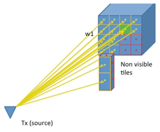
Figure 1.
Automatic ray splitting using discrete ray launching.
2.3. Visibility Preprocessing
Even more relevant is the following advantage. After the first bounce, RL must iterate the procedure, i.e., must propagate each bounced ray from each tile and look for further “visible” tiles to determine other bounces: here the source is no longer the Tx but virtual sources corresponding to each bouncing-tile. If the algorithm is discrete, virtual sources can be assumed corresponding to tile centers for the sake of visibility verification: by doing so, the determination of further bounces (or bouncing tiles) can be pre-calculated for a given environment, as visibility between tile centers does not depend on the current position of the Tx. The preliminary computation of visibility between all possible couples of tiles for a given environment can be called “visibility preprocessing”: although time consuming, it is performed only once for a given building database and visibility relations between tiles are stored in a “visibility matrix” for use in every future run for the same environment. Of course, for reflection or diffraction, where the actual visibility cone after the interaction actually depends on the virtual Tx, and therefore indirectly on the original Tx, visibility relations in the visibility matrix must be filtered according to the actual visibility cone, but the computation time advantage over traditional a-posteriori techniques is still present because the set of rays to be considered and filtered is already much smaller than the unrestricted set of potential rays [21].
2.4. Field Computation
Another important feature that makes the DED-RL algorithm computationally efficient is that, by being environment-driven, the tiles are both “bouncing-tiles” and the “points of arrival” where the field is computed. In other terms, the ray tubes are launched from the transmitter towards the visible tiles, and the incident field on them is computed and recorded, in order to achieve a complete field prediction map on all surfaces. Then, bounced ray tubes are generated from all of them towards other visible tiles using the visibility matrix, which stores all the tiles visible from the incident tiles, and then applying the proper reflection, diffraction, or scattering coefficient. Reflected and diffracted fields are computed with the usual Geometrical Optics (GO) [1] and Uniform Theory of Diffraction (UTD) [2] coefficients, while diffuse scattering is computed according to the Effective Roughness (ER) model [27], whose main parameter is the scattering coefficient S, corresponding to the percentage of power scattered in all directions at expenses of specular reflection. Diffraction is computed only for the “edge tiles”. Every time a tile is hit by a new ray tube, the computed field on its center is updated; if the field strength contribution on a tile falls below a given minimum threshold, the incident field is summed with the one already present on the tile, but the ray tube is no longer propagated with additional bounces. Fields are computed and summed in a fully coherent way, taking into account phases and polarization, and also cross-polarization introduced by some interaction mechanisms such as diffuse scattering [28].
In such a way, DED-RL allows a full 3D prediction on all the surfaces of the environment (i.e., ground, building walls, and roofs). An example of such 3D prediction is depicted in Figure 2 for a dense urban area located in the center of San Francisco.
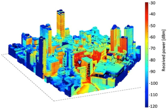
Figure 2.
Example of 3D radio coverage prediction in the San Francisco environment.
2.5. GPU Parallelization
Since the RL approach is inherently fit to parallel computing [16,21], the whole algorithm, including visibility preprocessing, has been parallelized for nVIDIA GPUs using the CUDA (Computer Unified Device Architecture) language extension, thus further reducing computation time with respect to traditional implementations. The CUDA platform is a software layer that gives direct access to the GPU’s computational elements (CUDA cores) and virtual instruction set for the execution of sets of parallel instructions (CUDA “kernels”) on nVIDIA GPU architectures.
CUDA processors are usually programmed in CUDA C/C++, which is basically the standard C/C++ programming language, with some CUDA extensions to handle parallel computation on multiple cores and threads [29].
2.6. Further Extensions to the DED-RL Algorithm
With respect to the algorithm presented in [21], the DED-RL features have been further extended in order to model:
- efficient Over-Rooftop (ORT) propagation through multiple diffractions over building rooftops;
- attenuation through vegetation;
- transmission through buildings at a limited extent, considering only the closest building to the Base Station (BS).
Regarding feature 1, it is well known that ORT diffraction is one of the dominant propagation mechanisms for the coverage of Non-Line-of-Sight (NLOS) locations when the BS is placed near or above the average rooftop level. In DED-RL, ORT diffraction is computed with a simplified approach using a multiple-screen UTD model limited to the vertical plane [2,4,5], considering one/two knife-edges for each building along the radial line between the BS and the receiving tiles. The ORT computation is performed for all the tiles that are not directly visible from the BS: since each ORT path is independent from the others, this computation is highly parallelizable, and is then implemented very efficiently on the GPU. Moreover, ORT rays are combined with reflection and scattering in a straightforward way, by using the visibility matrix: in fact, once a tile is reached from an ORT ray, the coverage can be extended through reflection/scattering to all the surrounding tiles that are directly visible from it.
Regarding feature 2, vegetated areas are modelled in a simplified way as “polygons” with a certain height, and then a ray-polygon intersection check is carried out every time a ray tube is launched from the BS, or a tile: the additional attenuation of the ray is then computed through multiplication of the ray length falling inside each polygon by a specific attenuation coefficient, expressed in dB/m [30].
Regarding feature 3, this mechanism can be very important for coverage of locations behind the Tx antenna, especially for microcellular sites when the BS is placed close to a corner of a building. In order to model transmission through the closest building from the BS, such a building is temporarily made “transparent” when finding the visible tiles from the BS: in such a way, those tiles that are obstructed by the building become automatically visible. After that, RL computation continues in the usual way with field computation and bouncing from all tiles, including the ones hidden by the building. Finally, only for the rays involving hidden tiles, an additional through-building attenuation is computed by the simplified formulas introduced in [31,32].
Figure 3 shows a simplified scheme describing the macrostructure of the model, including ORT and attenuation from vegetation, and the overall computation flow. A more detailed flow-chart of the algorithm can be found in [21].
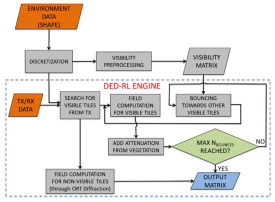
Figure 3.
Simplified scheme and computation flow of the DED-RL algorithm.
3. Validation
3.1. Measurement Campaigns
RF coverage measurements for both 2G and 4G cellular networks were collected in the cities of San Francisco, San José, and Atlanta. In San Francisco, several 2G cell sites, at the frequencies of 850 and 1900 MHz were chosen from all over the central part of the city. The cell site characteristics were derived from surveying each target site. BS antenna heights ranged from 6 to 100 m. Effective Radiated Power (ERP), which was found by using a scanner at Line-of-Sight (LOS) locations with each site, was generally between 30 and 45 dBm. Measurements were collected through drive tests, using a Rhode Schwarz scanner placed inside a minivan and a PCTEL OP178H omnidirectional antenna with 3 dBi gain placed on top of the minivan. The antenna height above the ground was approximately 1.8 m and exact Rx locations along routes were tracked using a combination of GPS, inertial devices, and speedometer. Using the scanner, the received signal strength indicator (RSSI) was recorded for the target broadcast control channels (BCCHs) as the minivan drove the streets around each cell site. From the recorded RSSI measurements, roughly 27,000 small-area average power measurements were extracted.
Measurements for San José and Atlanta (north and south) were collected in a very similar way as for San Francisco, after selecting several 4G Base Stations, and using a Rhode Schwarz TSME 4G scanner. Carrier frequencies were the same as in San Francisco, i.e., 850 and 1900 MHz. Due to the very vast measurement area, which encompasses 437 base station sites, ERP survey for each base station was not possible for San José and Atlanta, and since cellular operator ERP info were found unreliable—often lower than the actual figures—mean error statistics cannot be considered valid for San José and Atlanta (see next section).
3.2. Validation of the DED-RL Algorithm
As in [6] for the validation of a standard image RT algorithm, a subset of 18 sites in the San Francisco environment was selected in order to perform a comparative assessment of the overall performance of the new DED-RL algorithm vs. the traditional RT algorithm.
As one of the main sources of error in DED-RL is environment discretization, prediction accuracy has been analyzed for different tile sizes. RL simulations have been performed with the parameters shown in Table 1. As the DED-RL is discrete and allows the computation of the field only on discrete points upon surfaces (e.g., building walls and ground), the predicted field value on the closest ground tile has been considered for each drive-test measurement location.

Table 1.
Main settings for ray launching simulations.
Results in term of prediction error (mean value and standard deviation) as a function of the tile size in the San Francisco scenario are shown in Figure 4.
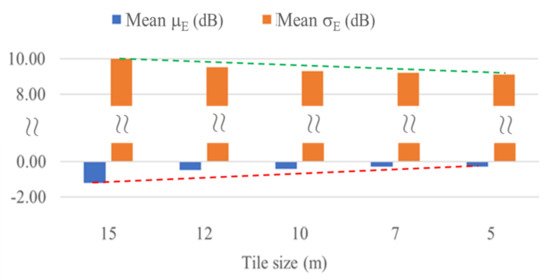
Figure 4.
Performance of the DED-RL in the San Francisco scenario (mean error and mean standard deviation of error w.r.t. measurements) for different tile sizes.
Prediction error “Erri” is computed as the predicted RSSI minus the measured RSSI for the generic, i-th test point. Then, mean error, μE and standard deviation of the error, σE are computed for the NRX locations covered by each cell site in the following way:
Global error statistics are finally derived computing the mean and the standard deviation of μE and σE for all the NBS cell sites:
These global statistics are shown more in detail for all the considered environments (San Francisco, San José, Atlanta) in the next sections.
Figure 4 shows that overall performance for San Francisco slightly improves when reducing the tile size, from very large tiles (15 × 15 m2), down to 5 × 5 m2: in particular, the global mean error () becomes very close to zero, while the average error standard deviation () reduces from 10 dB for the largest tiles, down to 9 dB, which is even better than what was obtained in [6]. This means that it is not necessary to consider very small tiles in order to achieve a good performance: this point is very important, as the amount of memory occupation (i.e., the size of the visibility matrix) and the computation time rapidly increase when reducing the tile size.
3.2.1. Comparison between DED-RL and RT
In Figure 5, the performance of DED-RL is compared to RT for the same 18 San Francisco’s cell sites considered in [6]: the standard deviation of the error w.r.t. measurements (σE) is reported for RT and DED-RL with x and y coordinates, respectively, while the red dashed line bisecting the xy-quadrant represents perfect correlation between the two models. Overall, the correlation between DED-RL and RT is evident, despite the fact that the two algorithms are different.
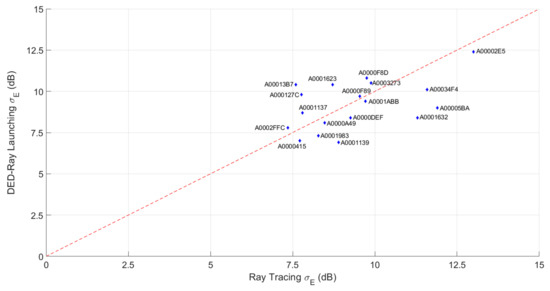
Figure 5.
Performance Comparison of DED-RL with image RT, in terms of error standard deviation (σE) for the 18 BS analyzed in [6]. 5 × 5 m2 tiles are considered in DED-RL simulations.
Looking at the results of DED-RL simulations, for the majority of sites, σE is below 10 dB, and for a few sites, σE has values between 7 and 8 dB. The latter one can be considered a very good result as San Francisco is a really challenging scenario due to the variety of the urban layout (alternation of residential areas, vegetated areas, dense urban areas with high-rise buildings) and the presence of hilly terrain [6].
One site with ID A00002E5 shows bad performance for both DED-RL and RT: this fact is probably due to recently constructed buildings close to the base station site that were not present in the building database. Other sites that show poor performance in DED-RL, namely A00013B7, A0001623, A000127C, A0000F8D, are all microcellular sites installed on buildings close to a street corner: in this case, small errors in base station location can yield large errors in the RF map, and probably DED-RL is more sensitive than RT to those errors due to environment discretization.
On the other hand, some other sites (A0001632, A0001139, A00005BA, A0001983, A00034F4) have better performance in DED-RL than in RT, while the performance of DED-RL and RT is very similar for all the remaining sites.
Some of the optimizations suggested in [8] have been applied also in DED-RL, in order to achieve a better performance. For example, for some sites located in hilly regions, the combination of ORT diffraction with scattering and reflection is very important to increase coverage in strongly-NLOS locations: this is the case of site A0002FFC, well described in [6]. After inserting the combination of scattering/reflection with ORT in the DED-RL simulation of site A0002FFC, the mean error (μE) reduced from −11.5 to −6 dB and the error standard deviation (σE) improved from 9.9 to 7.8 dB, thus confirming the findings already presented in [6].
Other sites are located in residential areas surrounded by vegetation, and in such cases, the results improve if vegetation polygons are properly modelled in the input database. This is the case of site A0000A49: after modelling vegetation, and assuming an attenuation of 0.04 dB/m (see Table 1) for the rays falling inside vegetation polygons, μE reduced from 6.5 to 0.3 dB, while σE improved from 8.8 to 8.4 dB.
Finally, for some sites near street corners, a better performance is obtained by enabling transmission through the building closest to the transmitting antenna: in this case, in fact, transmission through the corner is as important as diffraction for the signal to propagate in the side streets.
Global statistics in terms of mean error and error standard deviation for all 18 BS in San Francisco are shown in Table 2. On the average, the performance of the DED-RL is slightly better than RT, despite the discretization error, which is not present in image ray tracing algorithms. This is probably because DED-RL, being much more efficient, allows the simulation of a higher number of interactions (up to five bounces are considered in the present work) with respect to RT (up to three bounces considered in [6]).
Table 2.
Global statistics for the RL simulations vs. measurements in the San Francisco scenario. Global statistics of RT in the same scenario are reported as a reference.
3.2.2. Computation Time in the San Francisco Scenario
The average per-site computation time of DED-RL over all the 18 cell sites in San Francisco was of about 6 min, using a nVidia TESLA P100 Accelerator equipped with 3840 CUDA cores and 12 GB of GPU-RAM.
In DED-RL simulations, a full 10 km2 building map including the whole San Francisco downtown has been considered, differently from [6], where this map was simplified using an enhanced version of the simplification algorithm presented in [11], in order to achieve acceptable computation times with standard image ray tracing. For example, in [6] it is reported that for the site A000127C in San Francisco, the RT simulation time with the full 10 km2 map was of about 3.5 days, which was reduced to about 10 h by applying the map simplification algorithm.
On the other hand, the same site has been simulated using DED-RL using the full 10 km2 map—with no simplification—in 212 s, so in this case, the speed-up gain of DED-RL is of 1426x with respect to RT (212 s vs. 3.5 days): in other words, with DED-RL the computation time is reduced to about 3 min despite the fact that no map simplification was applied and a higher number of bounces was considered in the simulation (max five bounces in DED-RL, vs. max three bounces in RT). By applying the map simplification algorithm to DED-RL simulation of site A000127C, the computation time is further reduced to 145 s, and the speed-up gain increases to 2085x. These huge speed-ups are in line with the analysis shown in [21] for a benchmark scenario. Results for site A000127C are summarized in Table 3. Similar results have been obtained for the other sites in San Francisco, not reported here for brevity.
Table 3.
Comparison of computation time and speed-up gain of DED-RL vs. ray tracing for site A000127C in the San Francisco scenario.
3.2.3. Results for San José and Atlanta
Table 4 shows a comparison of measurements and RL simulations for the 437 sites cell sites in Atlanta and San José.
Table 4.
Global statistics for the RL simulations vs. Measurements in The San José and Atlanta scenarios.
In the table, mean error (μE) statistics are shaded in gray because they have low relevance, as nominal ERP values declared by the cellular operators turned out to be unreliable and exhaustive ERP survey was not possible. In particular, the nominal values were overestimated in several cases, so an unbiasing procedure was applied to the simulation results: this explains why the average μE values before unbiasing in Table 4 are quite high and always positive.
Regarding the error standard deviation (σE), performance is better than for San Francisco, especially for San José, which is a more standard urban scenario, with a nearly flat terrain, and a preponderance of mid-size buildings with vegetated areas: Figure 6 shows a comparison of the measured and simulated RF coverage map for one of the 79 sites in San José. The vegetated areas were available in the San José database, represented as brown polygons in Figure 6, and through-vegetation attenuation was taken into account as in [30]. The average per-site computation time for San José was 2.5 min, shorter than for San Francisco. The computation times for the Atlanta scenario (north and south) were similar to those of San Francisco (about 7 min per-site).
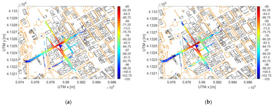
Figure 6.
Comparison of (a) measurements and (b) RL simulations for measurement site n. 40 in San José: in this case σE = 6.5 dB.
3.2.4. Wideband Results
The ray launcher’s temporal accuracy was verified using Timing Advance (TA) ranging measurements collected from 4G LTE testing devices in the San José scenario.
In LTE and 5G NR, TA is proportional to the roundtrip time between a base station (e.g., eNB, gNB) and user equipment (e.g., smartphones, IoT devices). A TA measurement can be converted to a ranging or Time of Arrival (ToA) measurement by removing timing offsets due to hardware components (e.g., wires) and digital components (e.g., filters), and dividing the remainder by two. In LTE, the ranging resolution is equal to 8 TS or 78.1 m, where TS is the basic timing unit [33]. Note that regular off the shelf handsets (e.g., Nexus 5X) will have the 8 TS ranging resolution. Though, special testing handsets (e.g., Samsung S5) can measure TA-based range at a finer resolution of 1 TS.
LTE TA measurements were collected using a Google Nexus 5X phone and a Samsung S5 phone. For a particular pair of base station and handset measurement location, TA measurements were collected and aggregated together temporally and spatially within a small radius around the central location. The variability in the aggregated TA and the corresponding ranging measurements is dependent on the multipath characteristics, which was then compared to ray launching predictions. Note that the TA of the first arrival, TA1, was used to remove the timing offsets in the aforementioned TA estimates by subtracting the following quantity from them:
where TAR is the TA of the shortest possible path, that was the LOS or quasi-LOS path in the considered cases.
ΔTA = TA1 − TAR
The resulting TA estimates divided by two are compared with DED-RL-predicted channel impulse responses, plotted with red impulses in Figure 7, where bars are used to indicate the ToA estimates (blue) and the corrected ToA values (green), where the bar width indicates the ranging resolution. Note that, for each measurement, there are two estimates, corresponding to the first and to the second arrival. The match between ray launching impulses and the corrected TA ranges is generally good, with a good matching between the first- and second-arrival ray clusters and the corresponding green bars.

Figure 7.
Comparison between TA measurements in San José and Power-Delay Profiles generated by DED-RL (a) for Samsung S5 device and (b) for Nexus 5X device.
4. Application Prospects
4.1. Application to UAV-Aided Wireless Networks
Future wireless networks will need to be much more flexible than in the past and they should be able to react smoothly and automatically to the fast time–space variations of any traffic demand. This can be achieved by moving part of the network infrastructure and tailor it according to actual traffic needs. Thanks to the ability to fly almost freely anywhere and whenever the highest needs arise, aerial platforms like Unmanned Aerial Vehicles (UAVs) become excellent candidates as nodes of future networks.
Recent studies on UAVs and their use as Aerial Base Stations (ABSs) [34] show that they might be an efficient complement to traditional Terrestrial Base Stations (TBSs) especially in case of events such as concerts and sport events, traffic jams, and disaster-recovery applications [35].
In order to properly deploy a heterogeneous network composed of both TBSs and ABSs, it is required to design and optimize the UAV trajectories so that the coverage is maximized, and the network should also be able to quickly reconfigure itself when the traffic demand abruptly increases in some areas. To accomplish this objective, a thorough ad accurate characterization of the air-to-ground radio channel is needed, as simple empirical channel models are not suitable, especially in dense urban areas where only a deterministic prediction is able to address the actual coverage in a realistic manner: this can be achieved in a straightforward way through the DED-RL software, which is able to generate hundreds or thousands of coverage maps of urban areas in a short time, thanks to its computational efficiency.
An example of radio coverage map obtained with DED-RL is shown in Figure 8, assuming that the ABS is flying over the historical center of the Italian city of Bologna at 150 m of altitude, and illuminates the ground with a directive antenna, whose half-power beamwidth is 80°. In this case, only the coverage at ground (i.e., along the streets) is represented, in order to make the urban structure visible, but DED-RL is able to deliver full-3D prediction also on the buildings surfaces, as explained before. It is worth noting that in dense urban areas like the one depicted here, the coverage map has not necessarily a circular or quasi-circular symmetry, like in rural or suburban areas. Therefore, in urban environments the obstruction of tall buildings and the combination of several propagation mechanisms, including reflection, diffraction, and scattering, is very important to predict the UAV-to-ground coverage in a realistic way, differently from rural/suburban areas where LOS is the largely dominant, if not the only, propagation mechanism [20].
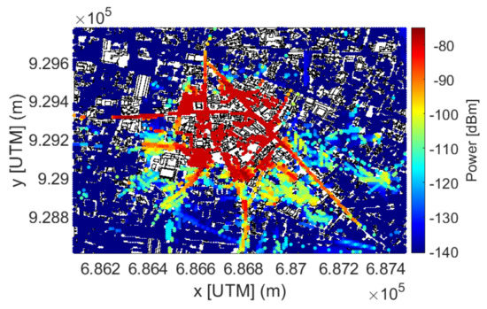
Figure 8.
Example of coverage map at ground of an UAV flying over an urban area, generated with the DED-RL. UAV height: 150 m. The ABS antenna is pointed towards ground with a half-power-beamwidth of 80°.
Radio coverage maps generated with DED-RL can then be used ad inputs for the network controller with the aim to manage radio resources and plan ABSs trajectories based on the simulated received power a priori for different UAV positions. Further details about this procedure, and a preliminary assessment of the performance, are presented in [24].
4.2. Application to Fingerprinting Localization
Ray launching can simplify the deployment of wide area fingerprint-based localization as proposed by J. Li et al. [36]. Generally, in fingerprinting approaches, a device at an unknown location collects a set of measurements (e.g., RSS, ToA, etc.). These measurements are then compared to a database of RF measurements at known locations, i.e., “fingerprints”, to estimate the device location. In prior works, wide area databases of 2D fingerprints were generally collected from “war driving” [37], which is time consuming and usually limited to locations at or near streets. To enable 3D fingerprints and circumvent the high time and resource cost of measurement collection, RL can be used to predict fingerprints.
There are several open problems in the use of RL for fingerprinting localization, which are addressed or alluded to in [36]:
- Fingerprint density: How dense should the discretization for ray launching simulation be? There are computation time and memory storage concerns for greater densities. The use of very efficient algorithms such as DED-RL is mandatory to ease this problem.
- Fingerprint measurement types: The predicted rays from ray launching need to be further processed into emulated radio measurements. These measurements should be consistent with those available from the target radio standard. For example, in 3GPP Rel 16 [38], there are a variety of measurements introduced for positioning, which generally fall in the following categories: RSS, ToA, Direction of Arrival/Departure (DoA/DoD).
- Fingerprinting localization algorithm: How to fuse different measurements and compare them to the database of fingerprints in a way that is consistent with the propagation physics? The foregoing problem need to be properly addressed to make fingerprinting localization unfold its potential.
5. Conclusions
In this work, a GPU-parallelized ray-launching algorithm previously proposed in [21] is tested against a very large set of measurements to assess its accuracy and efficiency. The validation has been carried out for over 500 base station sites in dense urban areas, including the very challenging scenario of San Francisco, showing that the overall accuracy is very similar to that of a standard image ray tracing algorithm, in spite of a much lower computation time (more than three orders of magnitude). Moreover, by evaluating the results for different tile sizes, it is shown that the accuracy of the proposed algorithm has little dependence on the discretization of the environment.
Further results are presented in the Atlanta and San José scenarios, showing a generally good performance, also in terms of temporal accuracy.
An outlook with some potential applications of the proposed algorithm is finally provided, with particular reference to UAV-aided wireless networks and localization based on fingerprinting.
Author Contributions
Conceptualization, E.M.V., J.S.L. and V.D.-E.; Methodology, E.M.V. and V.D.-E.; Software, E.M.V.; Validation, E.M.V., J.S.L. and J.J.Z.; Resources, J.J.Z. and S.G; Data curation, J.J.Z.; Writing—original draft preparation, E.M.V.; Writing—review and editing, E.M.V., J.S.L., S.G. and V.D.-E.; Supervision, E.M.V. All authors have read and agreed to the published version of the manuscript.
Funding
This research received no external funding.
Institutional Review Board Statement
Not applicable.
Informed Consent Statement
Not applicable.
Data Availability Statement
Network and cell site data are protected by Non-Disclosure Agreement between the cellular operator and Polaris Wireless Inc. Cell site identifier used in this paper have no relation with actual identifiers used by the cellular operator.
Acknowledgments
This work has been carried out in the framework of a research collaboration between Polaris Wireless Inc. and the CIRI-ICT Industrial Knowledge Transfer Center, University of Bologna, Italy.
Conflicts of Interest
The authors declare no conflict of interest.
References
- Balanis, C. Advanced Engineering Electromagnetics; Wiley: Hoboken, NJ, USA, 1989. [Google Scholar]
- Kouyoumjian, R.G.; Pathak, P.H. A uniform GTD for an edge in a perfectly conducting surface. Proc. IEEE 1974, 62, 1448–1461. [Google Scholar] [CrossRef] [Green Version]
- Yun, Z.; Iskander, M.F. Ray Tracing for Radio Propagation Modeling: Principles and Applications. IEEE Access 2015, 3, 1089–1100. [Google Scholar] [CrossRef]
- Bertoni, H.L. Radio Propagation for Modern Wireless Systems; Prentice Hall: Upper Saddle River, NJ, USA, 2000. [Google Scholar]
- Corre, Y.; Lostanlen, Y. Three-Dimensional Urban EM Wave Propagation Model for Radio Network Planning and Optimization Over Large Areas. IEEE Trans. Veh. Technol. 2009, 58, 3112–3123. [Google Scholar] [CrossRef]
- Vitucci, E.M.; Degli-Esposti, V.; Fuschini, F.; Lu, J.S.; Barbiroli, M.; Wu, J.N.; Zoli, M.; Zhu, J.J.; Bertoni, H.L. Ray Tracing RF Field Prediction: An Unforgiving Validation. Int. J. Antennas Propag. 2015, 2015, 184608. [Google Scholar] [CrossRef] [Green Version]
- Rossi, J.-P.; Gabillet, Y. A mixed ray launching/tracing method for full 3-D UHF propagation modeling and comparison with wideband measurements. IEEE Trans. Antennas Propag. 2002, 50, 517–523. [Google Scholar] [CrossRef]
- Corre, Y.; Lostanlen, Y.; Le Helloco, Y. A new approach for radio propagation modeling in urban environment: Knife-edge diffraction combined with 2D ray-tracing. In Proceedings of the 55th IEEE Vehicular Technology Conference (VTC Spring 2002), Birmingham, AL, USA, 6–9 May 2002. [Google Scholar]
- Liang, G.; Bertoni, H.L. A new approach to 3-D ray tracing for propagation prediction in cities. IEEE Trans. Antennas Propag. 1998, 46, 853–863. [Google Scholar] [CrossRef] [Green Version]
- Hoppe, R.; Woelfle, G.; Wertz, P. Advanced ray-optical wave propagation modelling for urban and indoor scenarios. Eur. Trans. Telecommun. 2003, 14, 61–69. [Google Scholar] [CrossRef]
- Degli-Esposti, V.; Fuschini, F.; Vitucci, E.M.; Falciasecca, G. Speed-up techniques for ray tracing field prediction models. IEEE Trans. Antennas Propag. 2009, 57, 1469–1480. [Google Scholar] [CrossRef]
- He, D.; Ai, B.; Guan, K.; Wang, L.; Zhong, Z.; Kürner, T. The Design and Applications of High-Performance Ray-Tracing Simulation Platform for 5G and Beyond Wireless Communications: A Tutorial. IEEE Commun. Surv. Tutor. 2018, 21, 10–27. [Google Scholar] [CrossRef]
- Amich, M.; De Luca, P.; Fiscale, S. Accelerated implementation of FQSqueezer novel genomic compression method. In Proceedings of the 19th IEEE International Symposium on Parallel and Distributed Computing (ISPDC), Warsaw, Poland, 5–8 July 2020; pp. 158–163. [Google Scholar]
- De Luca, P.; Galletti, A.; Giunta, G.; Marcellino, L. Recursive filter based GPU algorithms in a Data Assimilation scenario. Elsevier J. Comput. Sci. 2021, 53, 101339. [Google Scholar]
- Liu, F.; Jansson, N.; Podobas, A.; Fredriksson, A.; Markidis, S. Accelerating Radiation Therapy Dose Calculation with Nvidia GPUs. arXiv 2021, arXiv:2103.09683. [Google Scholar]
- Tao, Y.; Lin, H.; Bao, H. GPU-Based Shooting and Bouncing Ray Method for Fast RCS Prediction. IEEE Trans. Antennas Propag. 2010, 58, 494–502. [Google Scholar]
- Schiller, M.; Knoll, A.; Mocker, M.; Eibert, T. GPU accelerated ray launching for high-fidelity virtual test drives of VANET applications. In Proceedings of the 2015 International Conference on High Performance Computing & Simulation (HPCS), Amsterdam, The Netherlands, 20–24 July 2015; pp. 262–268. [Google Scholar]
- Tan, J.; Su, Z.; Long, Y. A Full 3-D GPU-based Beam-Tracing Method for Complex Indoor Environments Propagation Modeling. IEEE Trans. Antennas Propag. 2015, 63, 2705–2718. [Google Scholar] [CrossRef]
- Dai, Z.; Watson, R.J. Accelerating a ray launching model using GPU with CUDA. In Proceedings of the 12th European Conference on Antennas and Propagation (EuCAP 2018), London, UK, 9–13 April 2018. [Google Scholar]
- Degli-Esposti, V.; Lu, J.S.; Vitucci, E.M.; Fuschini, F.; Barbiroli, M.; Blaha, J.; Bertoni, H.L. Efficient RF Coverage Prediction through a fully Discrete, GPU-Parallelized Ray-Launching model. In Proceedings of the 12th European Conference on Antennas and Propagation (EuCAP 2018), London, UK, 9–13 April 2018. [Google Scholar]
- Lu, J.S.; Vitucci, E.M.; Degli-Esposti, V.; Fuschini, F.; Barbiroli, M.; Blaha, J.; Bertoni, H.L. A Discrete Environment-Driven GPU-Based Ray Launching Algorithm. IEEE Trans. Antennas Propag. 2019, 67, 1558–2221. [Google Scholar] [CrossRef]
- Egea-Lopez, E.; Losilla, F.; Pascual-Garcia, J.; Molina-Garcia-Pardo, J.-M. Vehicular Networks Simulation with Realistic Physics. IEEE Access 2019, 7, 44021–44036. [Google Scholar] [CrossRef]
- Arpaio, M.J.; Vitucci, E.M.; Barbiroli, M.; Degli-Esposti, V.; Masotti, D.; Fuschini, F. A Multi-Frequency Investigation of Air-To-Ground Urban Propagation Using a GPU-based Ray Launching Algorithm. IEEE Access 2021, 9, 54407–54419. [Google Scholar] [CrossRef]
- Mignardi, S.; Arpaio, M.J.; Buratti, C.; Vitucci, E.M.; Fuschini, F.; Verdone, R. Performance Evaluation of UAV-Aided Mobile Networks by Means of Ray Launching Generated REMs. In Proceedings of the 30th International Telecommunication Networks and Applications Conference (ITNAC 2020), Melbourne, Australia, 25–27 November 2020. [Google Scholar]
- Järveläinen, J.; Haneda, K.; Karttunen, A. Indoor Propagation Channel Simulations at 60 GHz Using Point Cloud Data. IEEE Trans. Antennas Propag. 2016, 64, 4457–4467. [Google Scholar] [CrossRef]
- Pang, M.; Wang, H.; Lin, K.; Lin, H. A GPU-Based Radio Wave Propagation Prediction with Progressive Processing on Point Cloud. IEEE Antennas Wirel. Propag. Lett. 2021, 20, 1078–1082. [Google Scholar] [CrossRef]
- Degli-Esposti, V.; Fuschini, F.; Vitucci, E.M.; Falciasecca, G. Measurement and modelling of scattering from buildings. IEEE Trans. Antennas Propag. 2007, 55, 143–153. [Google Scholar] [CrossRef]
- Degli-Esposti, V.; Kolmonen, V.-M.; Vitucci, E.M.; Fuschini, F.; Vainikainen, P. Analysis and ray tracing modelling of co- and cross-polarization radio propagation in urban environment. In Proceedings of the 2nd European Conference on Antennas and Propagation (EuCAP 2007), Edinburgh, UK, 11–18 November 2007. [Google Scholar]
- Soyata, T. GPU Parallel Program Development Using CUDA; CRC Press: Boca Raton, FL, USA, 2018. [Google Scholar]
- Vitucci, E.M.; Degli-Esposti, V.; Mani, F.; Fuschini, F.; Barbiroli, M.; Gan, M.; Li, C.; Zhao, J.; Zhong, Z. Tuning Ray Tracing for Mm-wave Coverage Prediction in Outdoor Urban Scenarios. Radio Sci. 2019, 54, 1112–1128. [Google Scholar] [CrossRef]
- Degli-Esposti, V.; Falciasecca, G.; Fuschini, F.; Vitucci, E.M. A meaningful indoor path-loss formula. IEEE Antennas Wirel. Propag. Lett. 2013, 12, 872–875. [Google Scholar] [CrossRef]
- Degli-Esposti, V.; Lu, J.S.; Wu, J.N.; Zhu, J.J.; Blaha, J.A.; Vitucci, E.M.; Fuschini, F.; Barbiroli, M. A Semi-Deterministic Model for Outdoor-to-Indoor Prediction in Urban Areas. IEEE Antennas Wirel. Propag. Lett. 2017, 16, 2412–2415. [Google Scholar] [CrossRef]
- 3GPP. Evolved Universal Terrestrial Radio Access (E-UTRA): Physical Layer Procedures; Document TS36.213 V9.0.1; 3GPP: 2010. Available online: https://www.etsi.org/deliver/etsi_ts/136200_136299/136213/09.00.01_60/ts_136213v090001p.pdf (accessed on 15 March 2021).
- Zeng, Y.; Zhang, R.; Lim, T.J. Wireless Communications with Unmanned Aerial Vehicles: Opportunities and Challenges. IEEE Commun. Mag. 2016, 54, 36–42. [Google Scholar] [CrossRef] [Green Version]
- Mohammed, F.; Idries, A.; Mohamed, N.; Al-Jaroodi, J.; Jawhar, I. UAVs for smart cities: Opportunities and challenges. In Proceedings of the 2014 International Conference on Unmanned Aircraft Systems (ICUAS), Orlando, FL, USA, 27–30 May 2014; pp. 267–273. [Google Scholar]
- Li, J.; Lu, I.; Lu, J.S. Hybrid Fingerprinting and Ray Extension Localization in NLOS Regions, Part I: Algorithm Development. Unpublished work. 2021. [Google Scholar]
- Vo, Q.D.; De, P. A survey of fingerprint-based outdoor localization. IEEE Commun. Surv. Tutor. 2015, 18, 491–506. [Google Scholar] [CrossRef]
- 3GPP. Stage 2 Functional Specification of User Equipment (UE) Positioning in NG-RAN, 3rd ed.; Version 16.3.0. TS 38.305; Generation Partnership Project (3GPP): 2020. Available online: https://www.3gpp.org/ftp//Specs/archive/38_series/38.305/38305-g30.zip (accessed on 15 March 2021).
Publisher’s Note: MDPI stays neutral with regard to jurisdictional claims in published maps and institutional affiliations. |
© 2021 by the authors. Licensee MDPI, Basel, Switzerland. This article is an open access article distributed under the terms and conditions of the Creative Commons Attribution (CC BY) license (https://creativecommons.org/licenses/by/4.0/).