
An Adaptive Protection Scheme for Coordination of Distance and Directional Overcurrent Relays in Distribution Systems Based on a Modified School-Based Optimizer

 ,
,  ,
,  ,
, 
Abstract
:1. Introduction
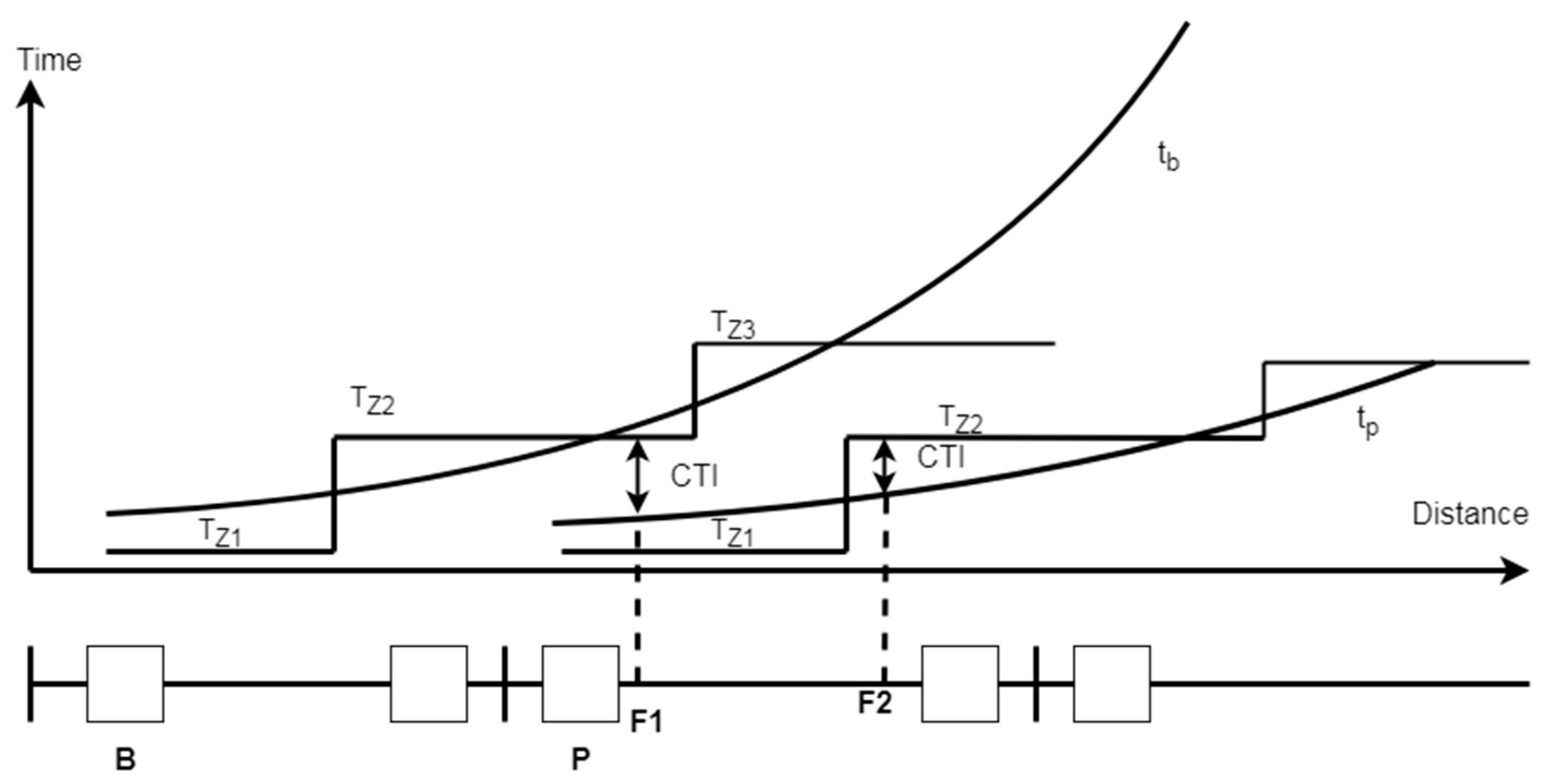
- An adaptive protection scheme was designed to coordinate both DOCRs and distance relays. This paper is the first one that deals with this problem in APS, as a solution to the DG impact. The effect of distance relays complicates this coordination problem in the DOCR’s coordination process, in addition to the impact of DGs.
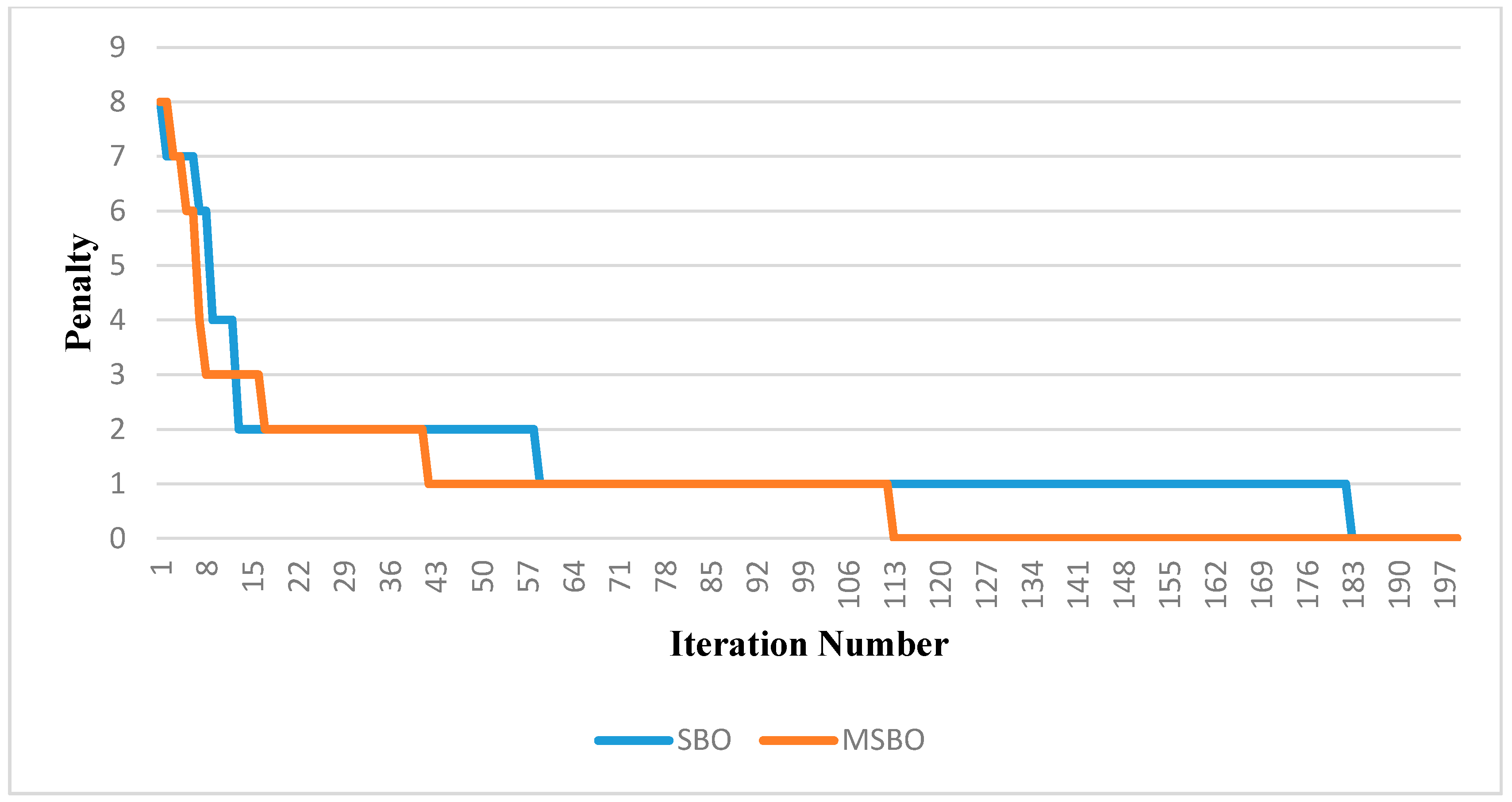
- The original SBO algorithm was modified to improve the response and convergence of the proposed algorithm. In doing so, two main points were modified, learning and the teacher-selected process. This algorithm could be effective in solving other power systems’ important topics, such as load frequency control, parameter estimation of the solar cell, optimal location, and the sizing of DGs.
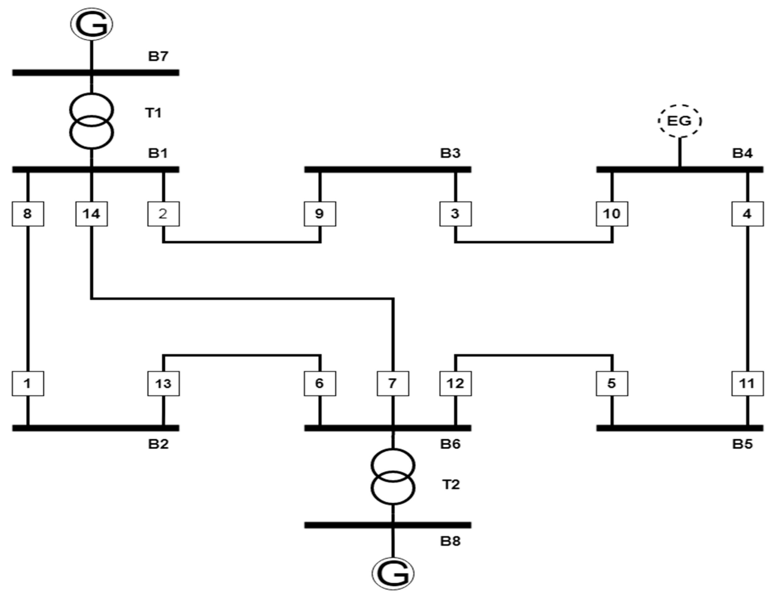
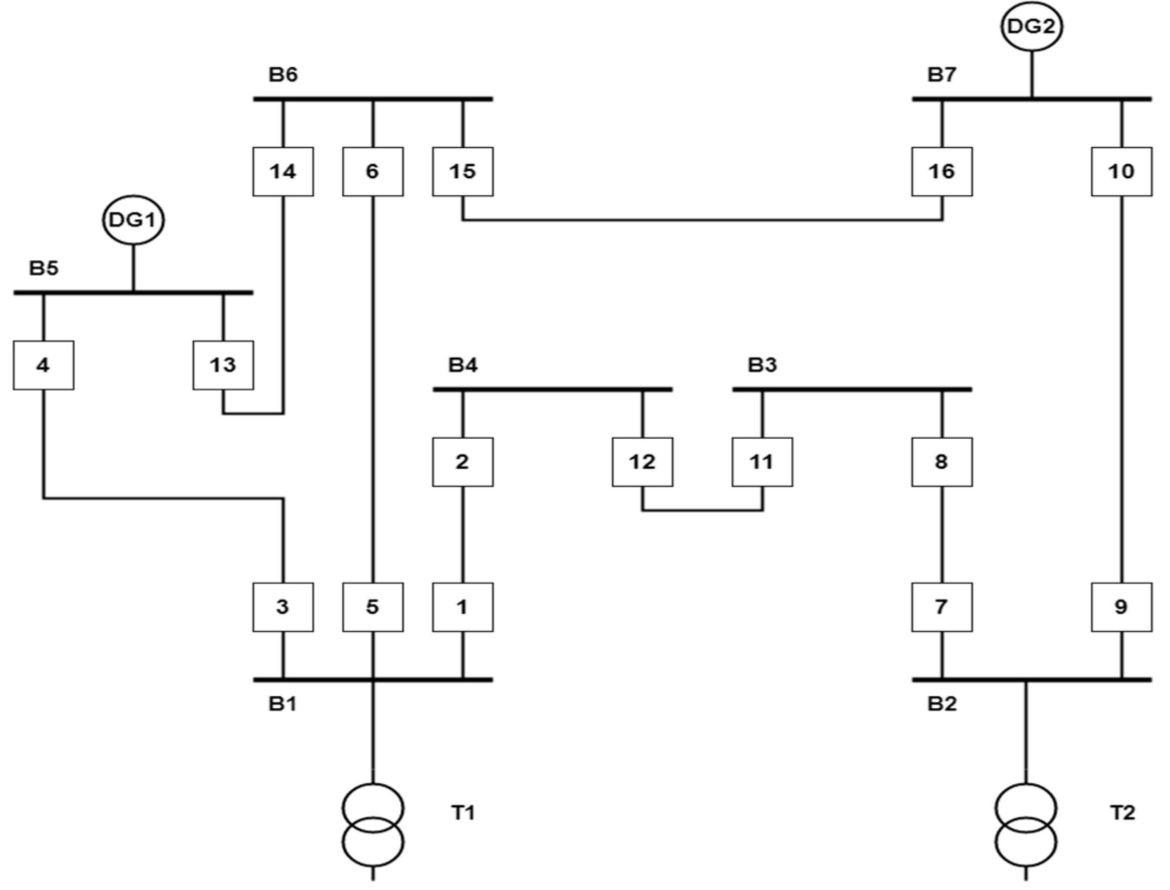
- The proposed protection system in this paper was tested on both IEEE 8-bus and IEEE 14-bus distribution networks, with the effect of DG’s on/off states.
2. The Mathematical Modelling of Coordination Problem
2.1. The Problem’s Limiters
2.2. The Problem’s Constraints
3. The Proposed Protection Scheme
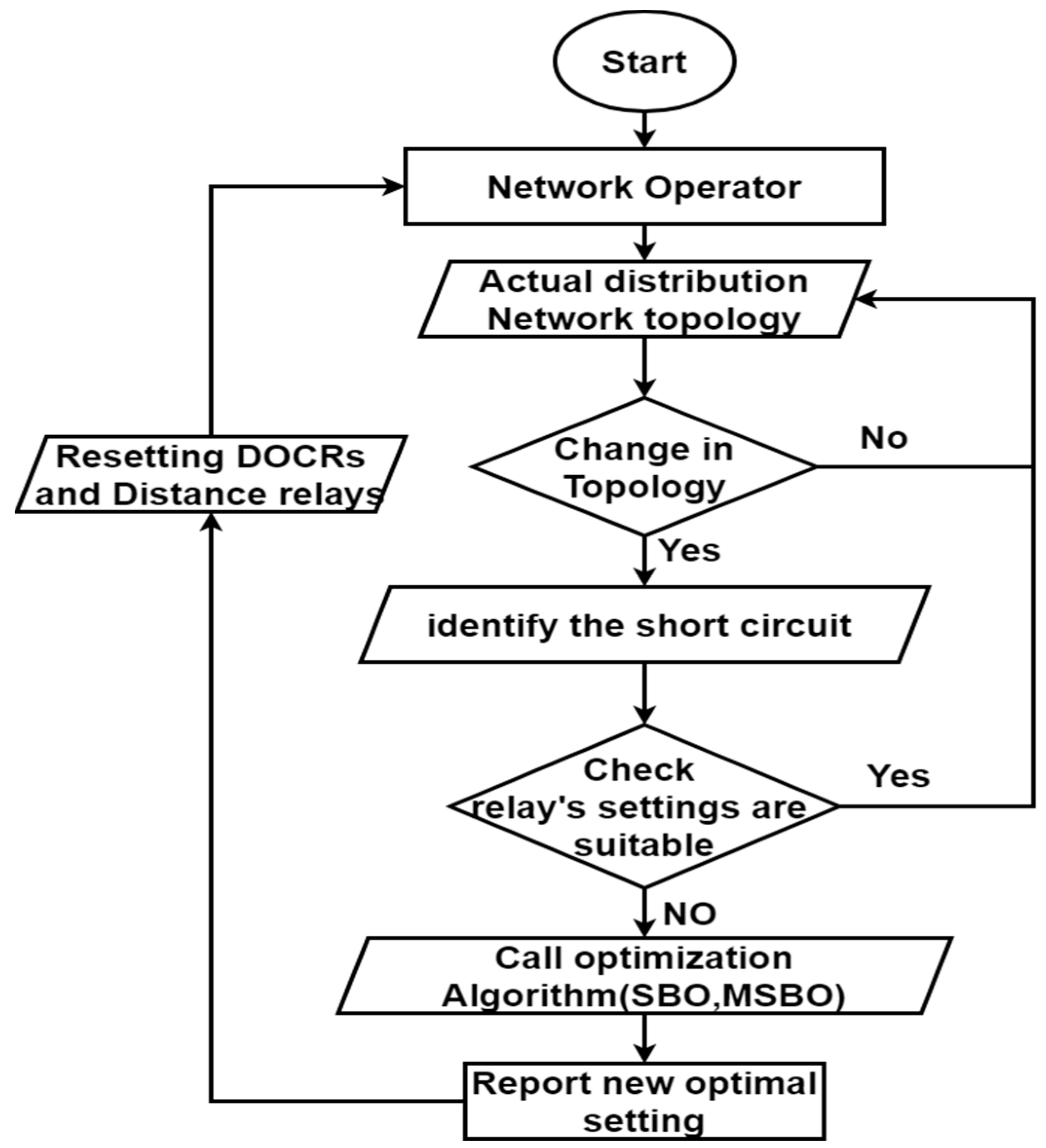
3.1. Smart Grid and Adaptive Protection Scheme (APS)
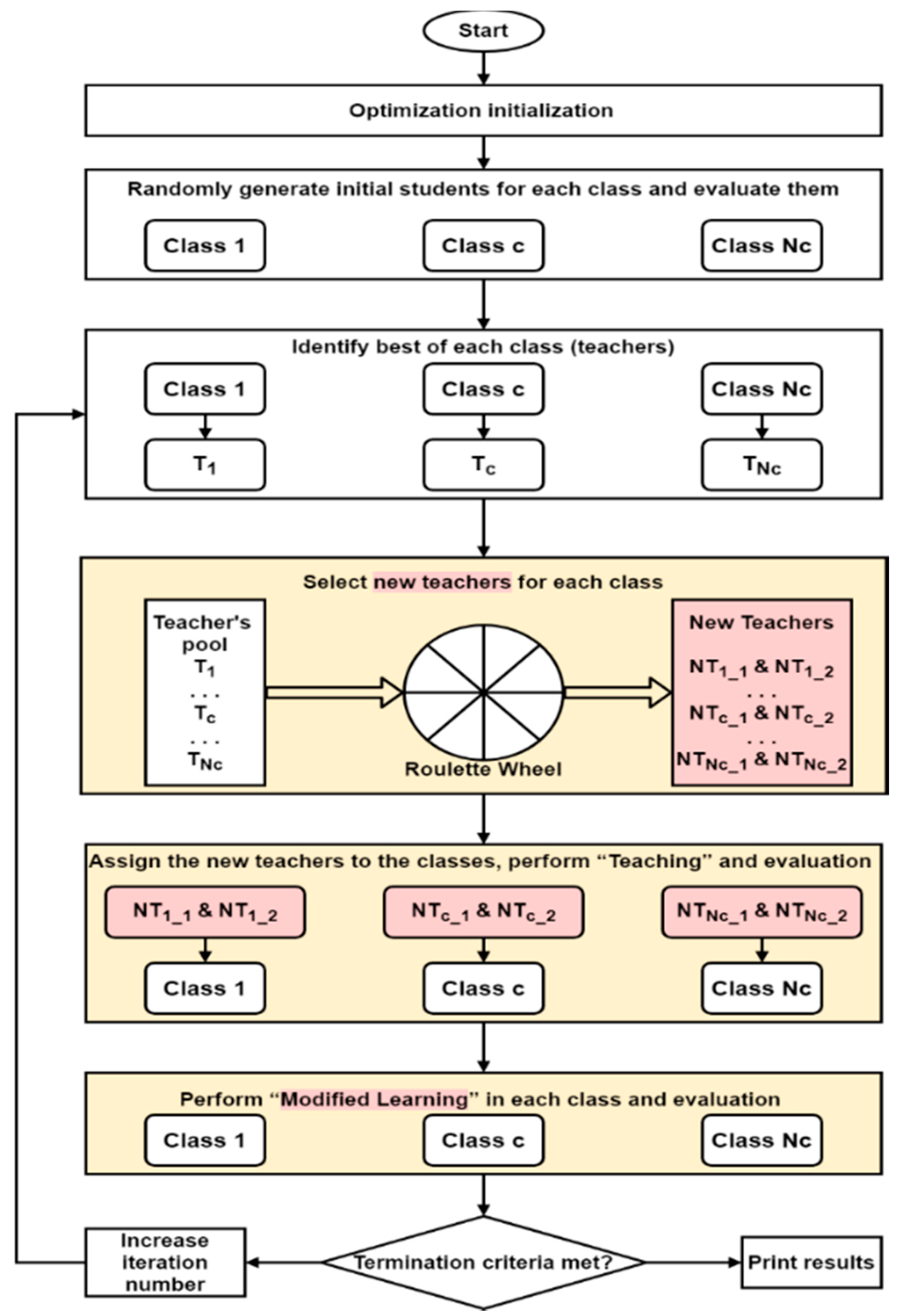
3.2. Original School-Based Optimization Algorithm
3.2.1. Teaching Phase
3.2.2. Learning Phase
- Randomly selected student p and another q while p ≠ q.
- If the fitness of student p is better than student q.
3.3. Modified SBO Algorithm
3.3.1. First Point: A Modified Learning Phase
- This step does not choose the student p randomly but as the place in the classroom.
- The student q is chosen randomly but not repeated with another student and cannot be equal to student p.
- Equations (18) and (19) are both applied and choosing the best value to compare with the student p fitness value (to replace or not).
3.3.2. Second Point: Teacher Selected
4. Results and Discussion
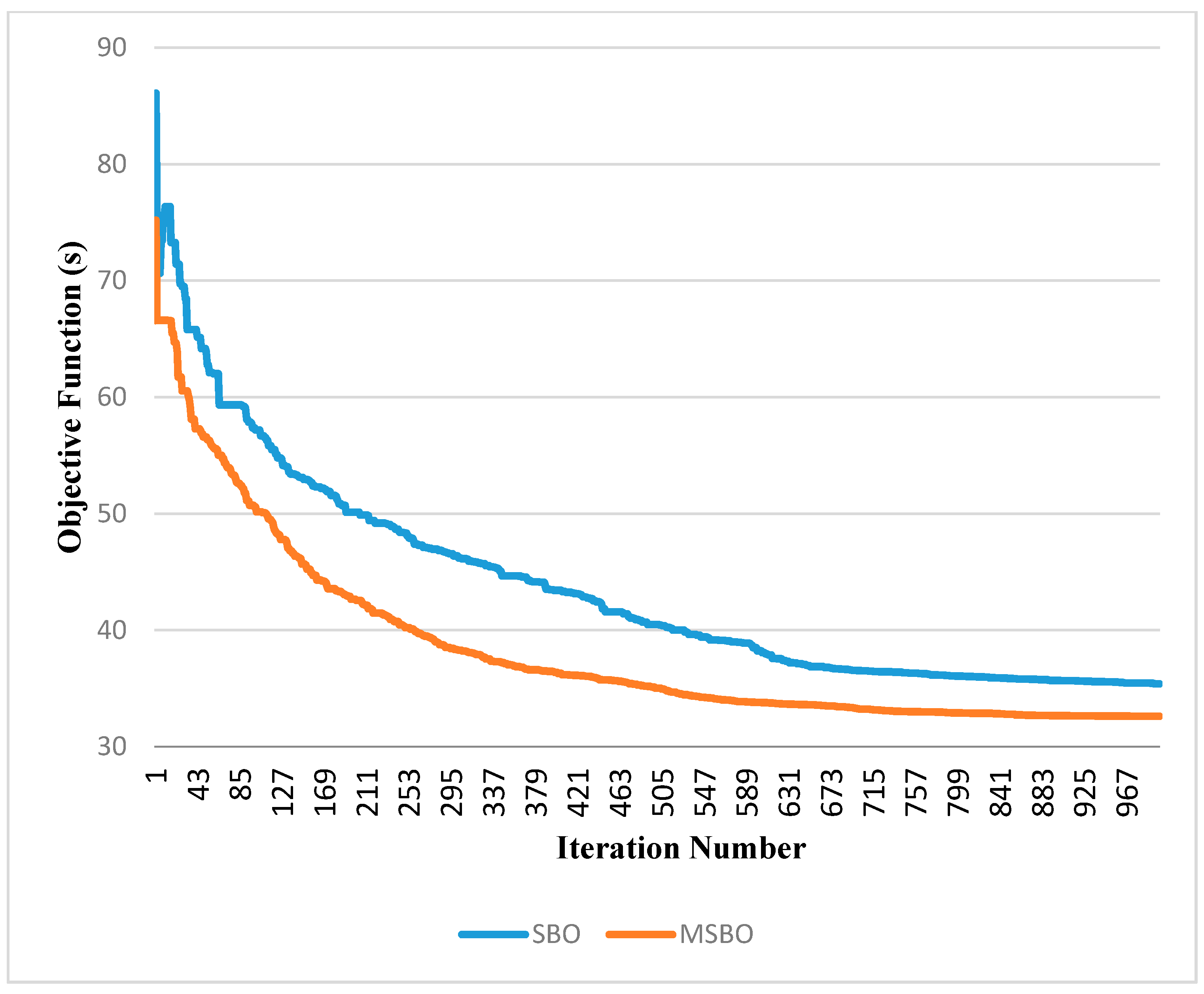
4.1. Test System I: IEEE 8-Bus Test System
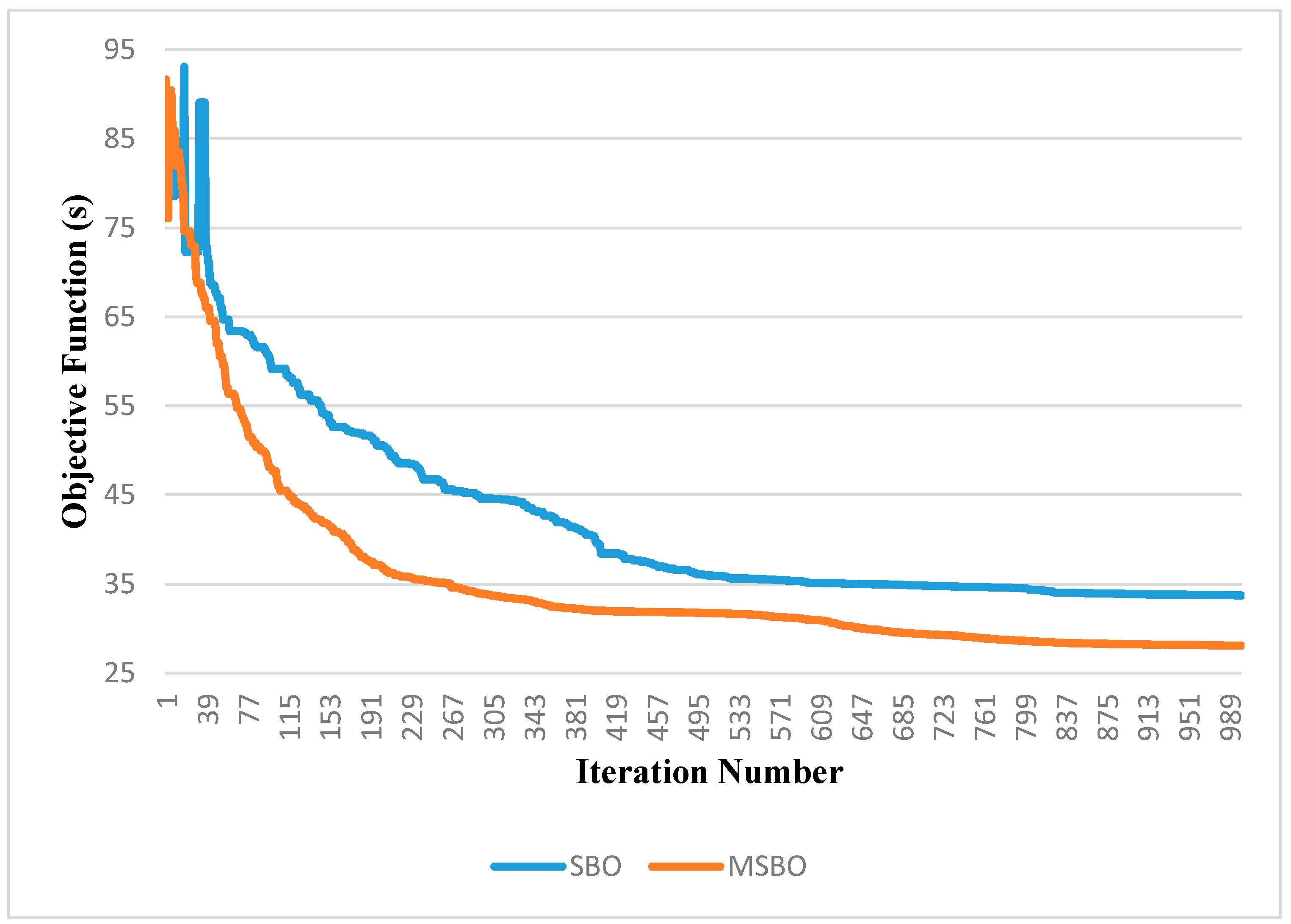
4.2. Test System II: IEEE 14-Bus Distribution Network
4.3. Varification of MSBO Using Etap 12.6.0
5. Conclusions
Author Contributions
Funding
Institutional Review Board Statement
Informed Consent Statement
Data Availability Statement
Conflicts of Interest
Appendix A

| Pair | Primary Relay | Back-Up Relay | Near-End | Far-End | ||
|---|---|---|---|---|---|---|
| Primary | Back-Up | Primary | Back-Up | |||
| 1 | 1 | 6 | 2703 | 2703 | 812 | 812 |
| 2 | 2 | 1 | 5390 | 812 | 3347 | 309 |
| 3 | 2 | 7 | 5390 | 1540 | 3347 | 586 |
| 4 | 3 | 2 | 3347 | 3347 | 2243 | 2243 |
| 5 | 4 | 3 | 2243 | 2243 | 1361 | 1361 |
| 6 | 5 | 4 | 1361 | 1361 | 416 | 416 |
| 7 | 6 | 5 | 4995 | 416 | 2703 | 20 |
| 8 | 6 | 14 | 4995 | 1540 | 2703 | 72 |
| 9 | 7 | 5 | 4267 | 416 | 1540 | REV |
| 10 | 7 | 13 | 4267 | 812 | 1540 | REV |
| 11 | 8 | 7 | 4995 | 1540 | 2507 | REV |
| 12 | 8 | 9 | 4995 | 416 | 2507 | REV |
| 13 | 9 | 10 | 1453 | 1453 | 416 | 416 |
| 14 | 10 | 11 | 2344 | 2344 | 1453 | 1453 |
| 15 | 11 | 12 | 3495 | 3495 | 2344 | 2344 |
| 16 | 12 | 13 | 5390 | 812 | 3495 | 348 |
| 17 | 12 | 14 | 5390 | 1540 | 3495 | 661 |
| 18 | 13 | 8 | 2507 | 2507 | 812 | 812 |
| 19 | 14 | 1 | 4267 | 812 | 1540 | REV |
| 20 | 14 | 9 | 4267 | 416 | 1540 | REV |
References
- Abdelhamid, M.; Kamel, S.; Mohamed, M.A.; Aljohani, M.; Rahmann, C.; Mosaad, M.I. Political Optimization Algorithm for Optimal Coordination of Directional Overcurrent Relays. In Proceedings of the 2020 IEEE Electric Power and Energy Conference (EPEC), Edmonton, AB, Canada, 9–10 November 2020; pp. 1–7. [Google Scholar] [CrossRef]
- Damchi, Y.; Sadeh, J.; Mashhadi, H.R. Considering pilot protection in the optimal coordination of distance and directional overcurrent relays. Iran. J. Electr. Electron. Eng. 2015, 11, 154–164. [Google Scholar]
- Perez, L.G.; Urdaneta, A.J. Optimal computation of distance relays second zone timing in a mixed protection scheme with directional overcurrent relays. IEEE Trans. Power Deliv. 2001, 16, 385–388. [Google Scholar] [CrossRef]
- Khederzadeh, M. Back-up protection of distance relay second zone by directional overcurrent relays with combined curves. In Proceedings of the 2006 IEEE Power Engineering Society General Meeting, Montreal, QC, Canada, 18–22 June 2006; p. 6. [Google Scholar] [CrossRef]
- Sarwagya, K.; Nayak, P.K.; Ranjan, S. Optimal coordination of directional overcurrent relays in complex distribution networks using sine cosine algorithm. Electr. Power Syst. Res. 2020, 187, 106435. [Google Scholar] [CrossRef]
- Ates, Y.; Uzunoglu, M.; Karakas, A.; Boynuegri, A.R.; Nadar, A.; Dag, B. Implementation of adaptive relay coordination in distribution systems including distributed generation. J. Clean. Prod. 2016, 112, 2697–2705. [Google Scholar] [CrossRef]
- Akdag, O.; Yeroglu, C. Optimal directional overcurrent relay coordination using MRFO algorithm: A case study of adaptive protection of the distribution network of the Hatay province of Turkey. Electr. Power Syst. Res. 2021, 192, 106998. [Google Scholar] [CrossRef]
- Mansour, M.M.; Mekhamer, S.F.; El-Kharbawe, N. A modified particle swarm optimizer for the coordination of directional overcurrent relays. IEEE Trans. Power Deliv. 2007, 22, 1400–1410. [Google Scholar] [CrossRef]
- Noghabi, A.S.; Sadeh, J.; Mashhadi, H.R. Considering different network topologies in optimal overcurrent relay coordination using a hybrid GA. IEEE Trans. Power Deliv. 2009, 24, 1857–1863. [Google Scholar] [CrossRef]
- Albasri, F.A.; Alroomi, A.R.; Talaq, J.H. Optimal coordination of directional overcurrent relays using biogeography-based optimization algorithms. IEEE Trans. Power Deliv. 2015, 30, 1810–1820. [Google Scholar] [CrossRef]
- Shih, M.Y.; Enriquez, A.C. Novel coordination of DOCRs using trigonometric differential evolution algorithm. IEEE Lat. Am. Trans. 2015, 13, 1605–1611. [Google Scholar] [CrossRef]
- Khurshaid, T.; Wadood, A.; Farkoush, S.G.; Kim, C.-H.; Yu, J.; Rhee, S.-B. Improved firefly algorithm for the optimal coordination of directional overcurrent relays. IEEE Access 2019, 7, 78503–78514. [Google Scholar] [CrossRef]
- Khurshaid, T.; Wadood, A.; Farkoush, S.G.; Yu, J.; Kim, C.-H.; Rhee, S.-B. An improved optimal solution for the directional overcurrent relays coordination using hybridized whale optimization algorithm in complex power systems. IEEE Access 2019, 7, 90418–90435. [Google Scholar] [CrossRef]
- Yu, J.; Kim, C.-H.; Rhee, S.-B. Oppositional jaya algorithm with distance-adaptive coefficient in solving directional over current relays coordination problem. IEEE Access 2019, 7, 150729–150742. [Google Scholar] [CrossRef]
- Korashy, A.; Kamel, S.; Alquthami, T.; Jurado, F. Optimal coordination of standard and non-standard direction overcurrent relays using an improved moth-flame optimization. IEEE Access 2020, 8, 87378–87392. [Google Scholar] [CrossRef]
- Abdelhamid, M.; Kamel, S.; Mohamed, M.A.; Rahmann, C. An Effective Approach for Optimal Coordination of Directional Overcurrent Relays Based on Artificial Ecosystem Optimizer. In Proceedings of the 2021 IEEE International Conference on Automation/XXIV Congress of the Chilean Association of Automatic Control (ICA-ACCA), Valparaíso, Chile, 22–26 March 2021; pp. 1–6. [Google Scholar] [CrossRef]
- Korashy, A.; Kamel, S.; Houssein, E.H.; Jurado, F.; Hashim, F.A. Development and application of evaporation rate water cycle algorithm for optimal coordination of directional overcurrent relays. Expert Syst. Appl. 2021, 185, 115538. [Google Scholar] [CrossRef]
- Marcolino, M.H.; Leite, J.B.; Mantovani, J.R.S. Optimal coordination of overcurrent directional and distance relays in meshed networks using genetic algorithm. IEEE Lat. Am. Trans. 2015, 13, 2975–2982. [Google Scholar] [CrossRef] [Green Version]
- Tiwari, R.; Singh, R.K.; Choudhary, N.K. A Comparative Analysis of Optimal Coordination of Distance and Overcurrent Relays with Standard Relay Characteristics using GA, GWO and WCA. In Proceedings of the 2020 IEEE Students Conference on Engineering & Systems (SCES), Prayagraj, India, 10–12 July 2020; pp. 1–6. [Google Scholar]
- Bangar, P.A.; Kalage, A.A. Optimum coordination of overcurrent and distance relays using JAYA optimization algorithm. In Proceedings of the 2017 International Conference on Nascent Technologies in Engineering (ICNTE), Vashi, India, 27–28 January 2017; pp. 1–5. [Google Scholar]
- Rivas, A.E.L.; Pareja, L.A.G.; Abrão, T. Coordination of distance and directional overcurrent relays using an extended continuous domain ACO algorithm and an hybrid ACO algorithm. Electr. Power Syst. Res. 2019, 170, 259–272. [Google Scholar] [CrossRef]
- Vijayakumar, D.; Nema, R.K. A novel optimal setting for directional over current relay coordination using particle swarm optimization. Int. J. Electr. Power Energy Syst. Eng. 2008, 1, 82. [Google Scholar]
- Singh, D.K.; Gupta, S. Optimal coordination of directional overcurrent relays: A genetic algorithm approach. In Proceedings of the 2012 IEEE Students’ Conference on Electrical, Electronics and Computer Science, Bhopal, India, 1–2 March 2012; pp. 1–4. [Google Scholar]
- Moirangthem, J.; Krishnanand, K.R.; Dash, S.S.; Ramaswami, R. Adaptive differential evolution algorithm for solving non-linear coordination problem of directional overcurrent relays. IET Gener. Transm. Distrib. 2013, 7, 329–336. [Google Scholar] [CrossRef]
- Shih, M.Y.; Salazar, C.A.C.; Enríquez, A.C. Adaptive directional overcurrent relay coordination using ant colony optimization. IET Gener. Transm. Distrib. 2015, 9, 2040–2049. [Google Scholar] [CrossRef]
- Chawla, A.; Bhalja, B.R.; Panigrahi, B.K.; Singh, M. Gravitational search based algorithm for optimal coordination of directional overcurrent relays using user defined characteristic. Electr. Power Compon. Syst. 2018, 46, 43–55. [Google Scholar] [CrossRef]
- Tjahjono, A.; Anggriawan, D.O.; Faizin, A.K.; Priyadi, A.; Pujiantara, M.; Taufik, T.; Purnomo, M.H. Adaptive modified firefly algorithm for optimal coordination of overcurrent relays. IET Gener. Transm. Distrib. 2017, 11, 2575–2585. [Google Scholar] [CrossRef]
- ElSayed, S.K.; Elattar, E.E. Hybrid Harris hawks optimization with sequential quadratic programming for optimal coordination of directional overcurrent relays incorporating distributed generation. Alex. Eng. J. 2021, 60, 2421–2433. [Google Scholar] [CrossRef]
- Farshchin, M.; Maniat, M.; Camp, C.V.; Pezeshk, S. School based optimization algorithm for design of steel frames. Eng. Struct. 2018, 171, 326–335. [Google Scholar] [CrossRef]
- Rao, R.V.; Savsani, V.J.; Vakharia, D.P. Teaching--learning-based optimization: A novel method for constrained mechanical design optimization problems. Comput. Aided Des. 2011, 43, 303–315. [Google Scholar] [CrossRef]
- Degertekin, S.O.; Tutar, H.; Lamberti, L. School-based optimization for performance-based optimum seismic design of steel frames. Eng. Comput. 2021, 37, 3283–3297. [Google Scholar] [CrossRef]
- Abdelghany, R.Y.; Kamel, S.; Ramadan, A.; Sultan, H.M.; Rahmann, C. Solar Cell Parameter Estimation Using School-Based Optimization Algorithm. In Proceedings of the 2021 IEEE International Conference on Automation/XXIV Congress of the Chilean Association of Automatic Control (ICA-ACCA), Valparaíso, Chile, 22–26 March 2021; pp. 1–6. [Google Scholar] [CrossRef]
- Sampaio, F.C.; Leão, R.P.S.; Sampaio, R.F.; Melo, L.S.; Barroso, G.C. A multi-agent-based integrated self-healing and adaptive protection system for power distribution systems with distributed generation. Electr. Power Syst. Res. 2020, 188, 106525. [Google Scholar] [CrossRef]
- Reis, F.B.d.; Pinto, J.O.C.P.; Reis, F.S.d.; Issicaba, D.; Rolim, J.G. Multi-agent dual strategy based adaptive protection for microgrids. Sustain. Energy Grids Netw. 2021, 27, 100501. [Google Scholar] [CrossRef]
- Cui, Q.; Weng, Y. An environment-adaptive protection scheme with long-term reward for distribution networks. Int. J. Electr. Power Energy Syst. 2020, 124, 106350. [Google Scholar] [CrossRef]
- Elmitwally, A.; Kandil, M.S.; Gouda, E.; Amer, A. Mitigation of DGs impact on variable-topology meshed network protection system by optimal fault current limiters considering overcurrent relay coordination. Electr. Power Syst. Res. 2020, 186, 106417. [Google Scholar] [CrossRef]
- Yazdaninejadi, A.; Nazarpour, D.; Golshannavaz, S. Sustainable electrification in critical infrastructure: Variable characteristics for overcurrent protection considering DG stability. Sustain. Cities Soc. 2020, 54, 102022. [Google Scholar] [CrossRef]
- Rajput, V.N.; Adelnia, F.; Pandya, K.S. Optimal coordination of directional overcurrent relays using improved mathematical formulation. IET Gener. Transm. Distrib. 2018, 12, 2086–2094. [Google Scholar] [CrossRef]
- Moravej, Z.; Ooreh, O.S. Coordination of distance and directional overcurrent relays using a new algorithm: Grey wolf optimizer. Turk. J. Electr. Eng. Comput. Sci. 2018, 26, 3130–3144. [Google Scholar] [CrossRef]
- Mohammadi, R.; Abyaneh, H.A.; Rudsari, H.M.; Fathi, S.H.; Rastegar, H. Overcurrent relays coordination considering the priority of constraints. IEEE Trans. Power Deliv. 2011, 26, 1927–1938. [Google Scholar] [CrossRef]
- Shih, M.Y.; Conde, A.; Ángeles-Camacho, C.; Fernández, E.; Leonowicz, Z.; Lezama, F.; Chan, J. A two stage fault current limiter and directional overcurrent relay optimization for adaptive protection resetting using differential evolution multi-objective algorithm in presence of distributed generation. Electr. Power Syst. Res. 2021, 190, 106844. [Google Scholar] [CrossRef]
- Camp, C.V.; Farshchin, M. Design of space trusses using modified teaching-learning based optimization. Eng. Struct. 2014, 62, 87–97. [Google Scholar] [CrossRef]
- Yang, M.-T.; Liu, A. Applying hybrid PSO to optimize directional overcurrent relay coordination in variable network topologies. J. Appl. Math. 2013, 2013, 879078. [Google Scholar] [CrossRef]
- Christie, R. Power systems test case archive. Electr. Eng. Dept. Univ. Wash. 2000, 108. Available online: https://labs.ece.uw.edu/pstca/ (accessed on 10 October 2021).
- Saleh, K.A.; Zeineldin, H.H.; Al-Hinai, A.; El-Saadany, E.F. Optimal coordination of directional overcurrent relays using a new time-current-voltage characteristic. IEEE Trans. Power Deliv. 2014, 30, 537–544. [Google Scholar] [CrossRef]


| Relay | Normal Topological Grid | With External DG | ||||||||||
|---|---|---|---|---|---|---|---|---|---|---|---|---|
| Original SBO | Modified SBO | Original SBO | Modified SBO | |||||||||
| TDS | IP | TZ2 | TDS | IP | TZ2 | TDS | IP | TZ2 | TDS | IP | TZ2 | |
| 1 | 0.194 | 174.94 | 1.07 | 0.164 | 191.56 | 0.984 | 0.193 | 229.12 | 1.108 | 0.119 | 370.20 | 1.037 |
| 2 | 0.287 | 289.93 | 1 | 0.198 | 528.22 | 0.936 | 0.274 | 353.42 | 1.013 | 0.168 | 723.15 | 0.928 |
| 3 | 0.332 | 80.55 | 0.875 | 0.252 | 137.37 | 0.815 | 0.236 | 242.43 | 0.928 | 0.143 | 549.25 | 0.903 |
| 4 | 0.125 | 318.77 | 0.793 | 0.128 | 249.02 | 0.719 | 0.173 | 393.64 | 0.86 | 0.158 | 438.72 | 0.84 |
| 5 | 0.1 | 235.55 | 1.425 | 0.1 | 158.21 | 0.917 | 0.114 | 434.09 | 0.974 | 0.1 | 500.20 | 0.993 |
| 6 | 0.175 | 654.44 | 1.049 | 0.286 | 120.14 | 0.823 | 0.216 | 389.94 | 0.9 | 0.297 | 140.18 | 0.843 |
| 7 | 0.297 | 147.82 | 1.068 | 0.208 | 247.29 | 0.982 | 0.205 | 443.09 | 1.174 | 0.369 | 80.03 | 0.991 |
| 8 | 0.257 | 226.38 | 0.931 | 0.128 | 725.52 | 0.916 | 0.303 | 420.07 | 1.258 | 0.269 | 205.83 | 0.884 |
| 9 | 0.1 | 173.26 | 0.994 | 0.1 | 145.66 | 0.861 | 0.314 | 127.59 | 1.174 | 0.256 | 143.03 | 1.039 |
| 10 | 0.136 | 389.05 | 0.913 | 0.155 | 171.41 | 0.698 | 0.227 | 455.43 | 1.121 | 0.177 | 552.63 | 1.012 |
| 11 | 0.274 | 196.10 | 0.954 | 0.123 | 578.75 | 0.805 | 0.147 | 784.60 | 1.13 | 0.154 | 666.46 | 1.049 |
| 12 | 0.382 | 167.49 | 1.053 | 0.166 | 631.70 | 0.869 | 0.227 | 595.26 | 1.052 | 0.317 | 295.35 | 1.055 |
| 13 | 0.198 | 191.93 | 1.146 | 0.226 | 120.34 | 1.011 | 0.165 | 271.95 | 1.088 | 0.167 | 284.74 | 1.127 |
| 14 | 0.233 | 282.76 | 1.147 | 0.128 | 460.94 | 0.935 | 0.264 | 243.24 | 1.089 | 0.321 | 173.52 | 1.123 |
| OF | 33.705 | 28.072 | 35.388 | 32.601 | ||||||||
| Pair | Near-End | Far-End | ||||||||||
|---|---|---|---|---|---|---|---|---|---|---|---|---|
| DOCRs | D&DOCR | DOCRs | D&DOCR | |||||||||
| Tp | Tb | CTI | Tp | TZ2B | CTI | Tp | Tb | CTI | Tp | TZ2P | CTI | |
| 1 | 0.423 | 0.623 | 0.200 | 0.423 | 0.823 | 0.400 | 0.784 | 1.027 | 0.243 | 0.784 | 0.984 | 0.2 |
| 2 | 0.582 | 0.784 | 0.202 | 0.582 | 0.984 | 0.402 | 0.736 | 2.390 | 1.655 | 0.736 | 0.936 | 0.2 |
| 3 | 0.582 | 0.782 | 0.200 | 0.582 | 0.982 | 0.400 | 0.736 | 1.674 | 0.939 | 0.736 | 0.936 | 0.2 |
| 4 | 0.535 | 0.736 | 0.200 | 0.535 | 0.936 | 0.400 | 0.615 | 0.943 | 0.329 | 0.615 | 0.815 | 0.2 |
| 5 | 0.399 | 0.615 | 0.216 | 0.399 | 0.815 | 0.416 | 0.519 | 0.752 | 0.233 | 0.519 | 0.719 | 0.2 |
| 6 | 0.318 | 0.519 | 0.201 | 0.318 | 0.719 | 0.401 | 0.717 | 1.738 | 1.021 | 0.717 | 0.917 | 0.2 |
| 7 | 0.517 | 0.717 | 0.201 | 0.517 | 0.917 | 0.401 | 0.623 | ــــــــ | ــــــــ | 0.623 | 0.823 | 0.2 |
| 8 | 0.517 | 0.735 | 0.218 | 0.517 | 0.935 | 0.418 | 0.623 | ــــــــ | ــــــــ | 0.623 | 0.823 | 0.2 |
| 9 | 0.497 | 0.717 | 0.220 | 0.497 | 0.917 | 0.420 | 0.782 | ــــــــ | ــــــــ | 0.782 | 0.982 | 0.2 |
| 10 | 0.497 | 0.811 | 0.314 | 0.497 | 1.011 | 0.514 | 0.782 | ــــــــ | ــــــــ | 0.782 | 0.982 | 0.2 |
| 11 | 0.457 | 0.782 | 0.325 | 0.457 | 0.982 | 0.525 | 0.716 | ــــــــ | ــــــــ | 0.716 | 0.916 | 0.2 |
| 12 | 0.457 | 0.661 | 0.203 | 0.457 | 0.861 | 0.403 | 0.716 | ــــــــ | ــــــــ | 0.716 | 0.916 | 0.2 |
| 13 | 0.298 | 0.498 | 0.200 | 0.298 | 0.698 | 0.400 | 0.661 | 1.216 | 0.555 | 0.661 | 0.861 | 0.2 |
| 14 | 0.405 | 0.605 | 0.200 | 0.405 | 0.805 | 0.400 | 0.498 | 0.924 | 0.426 | 0.498 | 0.698 | 0.2 |
| 15 | 0.469 | 0.669 | 0.200 | 0.469 | 0.869 | 0.400 | 0.605 | 0.877 | 0.272 | 0.605 | 0.805 | 0.2 |
| 16 | 0.532 | 0.811 | 0.280 | 0.532 | 1.011 | 0.480 | 0.669 | 1.471 | 0.802 | 0.669 | 0.869 | 0.2 |
| 17 | 0.532 | 0.735 | 0.203 | 0.532 | 0.935 | 0.403 | 0.669 | 2.480 | 1.811 | 0.669 | 0.869 | 0.2 |
| 18 | 0.504 | 0.716 | 0.212 | 0.504 | 0.916 | 0.412 | 0.811 | 7.976 | 7.165 | 0.811 | 1.011 | 0.2 |
| 19 | 0.394 | 0.784 | 0.389 | 0.394 | 0.984 | 0.589 | 0.735 | ــــــــ | ــــــــ | 0.735 | 0.935 | 0.2 |
| 20 | 0.394 | 0.661 | 0.266 | 0.394 | 0.861 | 0.466 | 0.735 | ــــــــ | ــــــــ | 0.735 | 0.935 | 0.2 |
| Pair | Near-End | Far-End | ||||||||||
|---|---|---|---|---|---|---|---|---|---|---|---|---|
| DOCRs | D&DOCR | DOCRs | D&DOCR | |||||||||
| Tp | Tb | CTI | Tp | TZ2B | CTI’ | Tp | Tb | CTI | Tp | TZ2P | CTI’ | |
| 1 | 0.378 | 0.643 | 0.265 | 0.378 | 0.843 | 0.465 | 0.837 | 1.041 | 0.204 | 0.837 | 1.037 | 0.2 |
| 2 | 0.548 | 0.839 | 0.291 | 0.548 | 1.037 | 0.489 | 0.728 | 13.984 | 13.256 | 0.728 | 0.928 | 0.2 |
| 3 | 0.548 | 0.793 | 0.244 | 0.548 | 0.991 | 0.443 | 0.728 | 1.131 | 0.404 | 0.728 | 0.928 | 0.2 |
| 4 | 0.527 | 0.728 | 0.200 | 0.527 | 0.928 | 0.400 | 0.703 | 1.029 | 0.325 | 0.703 | 0.903 | 0.2 |
| 5 | 0.503 | 0.703 | 0.201 | 0.503 | 0.903 | 0.401 | 0.640 | 1.537 | 0.897 | 0.640 | 0.840 | 0.2 |
| 6 | 0.440 | 0.640 | 0.200 | 0.440 | 0.840 | 0.400 | 0.793 | 1.088 | 0.295 | 0.793 | 0.993 | 0.2 |
| 7 | 0.531 | 0.793 | 0.262 | 0.531 | 0.993 | 0.462 | 0.643 | 3.115 | 2.472 | 0.643 | 0.843 | 0.2 |
| 8 | 0.531 | 0.923 | 0.392 | 0.531 | 1.123 | 0.592 | 0.643 | ــــــــ | ــــــــ | 0.643 | 0.843 | 0.2 |
| 9 | 0.593 | 0.793 | 0.200 | 0.593 | 0.993 | 0.400 | 0.791 | ــــــــ | ــــــــ | 0.791 | 0.991 | 0.2 |
| 10 | 0.593 | 0.928 | 0.335 | 0.593 | 1.127 | 0.534 | 0.791 | ــــــــ | ــــــــ | 0.791 | 0.991 | 0.2 |
| 11 | 0.537 | 0.793 | 0.256 | 0.537 | 0.991 | 0.454 | 0.684 | ــــــــ | ــــــــ | 0.684 | 0.884 | 0.2 |
| 12 | 0.537 | 0.839 | 0.302 | 0.537 | 1.039 | 0.502 | 0.684 | 1.308 | 0.624 | 0.684 | 0.884 | 0.2 |
| 13 | 0.611 | 0.812 | 0.201 | 0.611 | 1.012 | 0.401 | 0.839 | 1.656 | 0.817 | 0.839 | 1.039 | 0.2 |
| 14 | 0.622 | 0.849 | 0.227 | 0.622 | 1.049 | 0.427 | 0.812 | 2.002 | 1.190 | 0.812 | 1.012 | 0.2 |
| 15 | 0.619 | 0.855 | 0.236 | 0.619 | 1.055 | 0.436 | 0.849 | 1.049 | 0.200 | 0.849 | 1.049 | 0.2 |
| 16 | 0.719 | 0.928 | 0.209 | 0.719 | 1.127 | 0.408 | 0.855 | 2.770 | 1.914 | 0.855 | 1.055 | 0.2 |
| 17 | 0.719 | 0.923 | 0.204 | 0.719 | 1.123 | 0.404 | 0.855 | 1.423 | 0.568 | 0.855 | 1.055 | 0.2 |
| 18 | 0.485 | 0.685 | 0.200 | 0.485 | 0.884 | 0.399 | 0.927 | 1.182 | 0.255 | 0.927 | 1.127 | 0.2 |
| 19 | 0.639 | 0.839 | 0.200 | 0.639 | 1.037 | 0.398 | 0.923 | ــــــــ | ــــــــ | 0.923 | 1.123 | 0.2 |
| 20 | 0.639 | 0.839 | 0.200 | 0.639 | 1.039 | 0.400 | 0.923 | ــــــــ | ــــــــ | 0.923 | 1.123 | 0.2 |
| Relay | Normal Topological | With External DG | ||||||||||
|---|---|---|---|---|---|---|---|---|---|---|---|---|
| Original SBO | Modified SBO | Original SBO | Modified SBO | |||||||||
| TDS | IP | TZ2 | TDS | IP | TZ2 | TDS | IP | TZ2 | TDS | IP | TZ2 | |
| 1 | 0.223 | 235.93 | 1.246 | 0.214 | 157.86 | 0.984 | 0.386 | 392.93 | 1.549 | 0.384 | 337.37 | 1.442 |
| 2 | 0.11 | 185.11 | 0.885 | 0.159 | 149.46 | 1.028 | 0.37 | 188.60 | 1.455 | 0.209 | 314.56 | 1.153 |
| 3 | 0.135 | 232.94 | 0.931 | 0.155 | 164.17 | 0.858 | 0.434 | 139.04 | 1.255 | 0.241 | 465.02 | 1.243 |
| 4 | 0.156 | 51.91 | 1.103 | 0.232 | 20.02 | 0.937 | 0.376 | 52.32 | 1.455 | 0.402 | 39.28 | 1.376 |
| 5 | 0.243 | 80.15 | 0.824 | 0.211 | 142.21 | 0.895 | 0.492 | 231.73 | 1.514 | 0.289 | 394.61 | 1.18 |
| 6 | 0.361 | 28.91 | 1.069 | 0.219 | 63.82 | 0.937 | 0.356 | 131.99 | 1.454 | 0.621 | 28.58 | 1.407 |
| 7 | 0.241 | 140.62 | 0.865 | 0.164 | 425.78 | 1.025 | 0.731 | 71.12 | 1.446 | 0.33 | 361.09 | 1.172 |
| 8 | 0.258 | 60.58 | 0.953 | 0.15 | 117.13 | 0.815 | 0.447 | 106.48 | 1.367 | 0.283 | 233.98 | 1.266 |
| 9 | 0.105 | 308.66 | 0.864 | 0.162 | 197.06 | 0.923 | 0.349 | 347.18 | 1.423 | 0.363 | 260.94 | 1.308 |
| 10 | 0.121 | 187.97 | 1.162 | 0.116 | 167.35 | 1.014 | 0.311 | 239.60 | 1.566 | 0.447 | 72.25 | 1.299 |
| 11 | 0.158 | 176.02 | 0.854 | 0.282 | 85.18 | 1.008 | 0.529 | 119.67 | 1.414 | 0.324 | 209.62 | 1.121 |
| 12 | 0.229 | 150.99 | 1.294 | 0.165 | 133.91 | 0.93 | 0.534 | 105.85 | 1.499 | 0.569 | 69.66 | 1.398 |
| 13 | 0.151 | 101.59 | 1.077 | 0.185 | 58.68 | 0.929 | 0.399 | 85.44 | 1.345 | 0.464 | 60.89 | 1.362 |
| 14 | 0.205 | 65.11 | 0.8 | 0.313 | 27.29 | 0.861 | 0.46 | 54.40 | 1.088 | 0.444 | 58.67 | 1.078 |
| 15 | 0.136 | 179.69 | 0.953 | 0.139 | 152.58 | 0.878 | 0.489 | 106.17 | 1.38 | 0.298 | 276.49 | 1.297 |
| 16 | 0.119 | 201.72 | 1.092 | 0.198 | 89.52 | 0.984 | 0.491 | 102.67 | 1.494 | 0.4 | 141.69 | 1.408 |
| OF | 36.86 | 34.806 | 57.268 | 51.068 | ||||||||
| Pair | Near-End | Far-End | ||||||||||
|---|---|---|---|---|---|---|---|---|---|---|---|---|
| DOCRs | D&DOCR | DOCRs | D&DOCR | |||||||||
| Tp | Tb | CTI | Tp | TZ2B | CTI’ | Tp | Tb | CTI | Tp | TZ2P | CTI’ | |
| 1 | 0.537 | 0.737 | 0.201 | 0.537 | 0.937 | 0.401 | 0.784 | 1.096 | 0.312 | 0.784 | 0.984 | 0.2 |
| 2 | 0.537 | 0.737 | 0.201 | 0.537 | 0.937 | 0.401 | 0.784 | 1.272 | 0.488 | 0.784 | 0.984 | 0.2 |
| 3 | 0.575 | 0.808 | 0.233 | 0.575 | 1.008 | 0.433 | 0.828 | 1.032 | 0.203 | 0.828 | 1.028 | 0.2 |
| 4 | 0.374 | 0.828 | 0.455 | 0.374 | 1.028 | 0.655 | 0.658 | 1.997 | 1.339 | 0.658 | 0.858 | 0.2 |
| 5 | 0.374 | 0.737 | 0.364 | 0.374 | 0.937 | 0.564 | 0.658 | ــــ | ــــ | 0.658 | 0.858 | 0.2 |
| 6 | 0.427 | 0.661 | 0.234 | 0.427 | 0.861 | 0.434 | 0.737 | 1.907 | 1.169 | 0.737 | 0.937 | 0.2 |
| 7 | 0.504 | 0.828 | 0.325 | 0.504 | 1.028 | 0.525 | 0.695 | 1.352 | 0.657 | 0.695 | 0.895 | 0.2 |
| 8 | 0.504 | 0.737 | 0.234 | 0.504 | 0.937 | 0.434 | 0.695 | ــــ | ــــ | 0.695 | 0.895 | 0.2 |
| 9 | 0.524 | 0.729 | 0.204 | 0.524 | 0.929 | 0.404 | 0.737 | ــــ | ــــ | 0.737 | 0.937 | 0.2 |
| 10 | 0.524 | 0.784 | 0.259 | 0.524 | 0.984 | 0.459 | 0.737 | 0.938 | 0.201 | 0.737 | 0.937 | 0.2 |
| 11 | 0.613 | 0.814 | 0.2 | 0.613 | 1.014 | 0.4 | 0.825 | 1.546 | 0.721 | 0.825 | 1.025 | 0.2 |
| 12 | 0.529 | 0.73 | 0.201 | 0.529 | 0.93 | 0.401 | 0.615 | 0.856 | 0.241 | 0.615 | 0.815 | 0.2 |
| 13 | 0.413 | 0.615 | 0.202 | 0.413 | 0.815 | 0.402 | 0.723 | 7.393 | 6.669 | 0.723 | 0.923 | 0.2 |
| 14 | 0.476 | 0.676 | 0.2 | 0.476 | 0.878 | 0.403 | 0.814 | 1.703 | 0.89 | 0.814 | 1.014 | 0.2 |
| 15 | 0.621 | 0.825 | 0.204 | 0.621 | 1.025 | 0.404 | 0.808 | 1.604 | 0.796 | 0.808 | 1.008 | 0.2 |
| 16 | 0.54 | 0.784 | 0.244 | 0.54 | 0.984 | 0.444 | 0.73 | 1.066 | 0.336 | 0.73 | 0.93 | 0.2 |
| 17 | 0.452 | 0.658 | 0.205 | 0.452 | 0.858 | 0.405 | 0.729 | 2.547 | 1.819 | 0.729 | 0.929 | 0.2 |
| 18 | 0.495 | 0.695 | 0.2 | 0.495 | 0.895 | 0.4 | 0.661 | 2.583 | 1.922 | 0.661 | 0.861 | 0.2 |
| 19 | 0.495 | 0.784 | 0.289 | 0.495 | 0.984 | 0.489 | 0.661 | 1.187 | 0.526 | 0.661 | 0.861 | 0.2 |
| 20 | 0.391 | 0.695 | 0.304 | 0.391 | 0.895 | 0.504 | 0.678 | 1.445 | 0.766 | 0.678 | 0.878 | 0.2 |
| 21 | 0.391 | 0.729 | 0.337 | 0.391 | 0.929 | 0.537 | 0.678 | 1.66 | 0.982 | 0.678 | 0.878 | 0.2 |
| 22 | 0.522 | 0.723 | 0.201 | 0.522 | 0.923 | 0.401 | 0.784 | 1.886 | 1.102 | 0.784 | 0.984 | 0.2 |
| Pair | Near-End | Far-End | ||||||||||
|---|---|---|---|---|---|---|---|---|---|---|---|---|
| DOCRs | D&DOCR | DOCRs | D&DOCR | |||||||||
| Tp | Tb | CTI | Tp | TZ2B | CTI | Tp | Tb | CTI | Tp | TZ2P | CTI | |
| 1 | 0.973 | 1.18 | 0.207 | 0.973 | 1.376 | 0.403 | 1.242 | 1.871 | 0.629 | 1.242 | 1.442 | 0.2 |
| 2 | 0.973 | 1.205 | 0.232 | 0.973 | 1.407 | 0.434 | 1.242 | 2.081 | 0.839 | 1.242 | 1.442 | 0.2 |
| 3 | 0.718 | 0.921 | 0.203 | 0.718 | 1.121 | 0.403 | 0.953 | 1.159 | 0.207 | 0.953 | 1.153 | 0.2 |
| 4 | 0.644 | 0.956 | 0.312 | 0.644 | 1.153 | 0.509 | 1.043 | 1.508 | 0.464 | 1.043 | 1.243 | 0.2 |
| 5 | 0.644 | 1.205 | 0.562 | 0.644 | 1.407 | 0.763 | 1.043 | ــــ | ــــ | 1.043 | 1.243 | 0.2 |
| 6 | 0.677 | 0.881 | 0.204 | 0.677 | 1.078 | 0.401 | 1.176 | 26.389 | 25.213 | 1.176 | 1.376 | 0.2 |
| 7 | 0.752 | 0.956 | 0.204 | 0.752 | 1.153 | 0.401 | 0.98 | 1.506 | 0.525 | 0.98 | 1.18 | 0.2 |
| 8 | 0.752 | 1.18 | 0.428 | 0.752 | 1.376 | 0.624 | 0.98 | ــــ | ــــ | 0.98 | 1.18 | 0.2 |
| 9 | 0.948 | 1.162 | 0.214 | 0.948 | 1.362 | 0.414 | 1.207 | ــــ | ــــ | 1.207 | 1.407 | 0.2 |
| 10 | 0.948 | 1.206 | 0.258 | 0.948 | 1.408 | 0.46 | 1.207 | 1.409 | 0.202 | 1.207 | 1.407 | 0.2 |
| 11 | 0.873 | 1.1 | 0.227 | 0.873 | 1.299 | 0.427 | 0.972 | 1.323 | 0.351 | 0.972 | 1.172 | 0.2 |
| 12 | 0.947 | 1.181 | 0.234 | 0.947 | 1.398 | 0.451 | 1.066 | 1.271 | 0.205 | 1.066 | 1.266 | 0.2 |
| 13 | 0.832 | 1.059 | 0.227 | 0.832 | 1.266 | 0.433 | 1.108 | 3.803 | 2.695 | 1.108 | 1.308 | 0.2 |
| 14 | 0.892 | 1.097 | 0.205 | 0.892 | 1.297 | 0.405 | 1.099 | 1.821 | 0.722 | 1.099 | 1.299 | 0.2 |
| 15 | 0.768 | 0.972 | 0.204 | 0.768 | 1.172 | 0.404 | 0.921 | 1.22 | 0.299 | 0.921 | 1.121 | 0.2 |
| 16 | 1.038 | 1.242 | 0.204 | 1.038 | 1.442 | 0.404 | 1.198 | 1.611 | 0.413 | 1.198 | 1.398 | 0.2 |
| 17 | 0.826 | 1.032 | 0.206 | 0.826 | 1.243 | 0.417 | 1.162 | 6.046 | 4.884 | 1.162 | 1.362 | 0.2 |
| 18 | 0.691 | 0.98 | 0.29 | 0.691 | 1.18 | 0.49 | 0.878 | 2.43 | 1.553 | 0.878 | 1.078 | 0.2 |
| 19 | 0.691 | 1.206 | 0.515 | 0.691 | 1.408 | 0.717 | 0.878 | 1.489 | 0.612 | 0.878 | 1.078 | 0.2 |
| 20 | 0.766 | 0.98 | 0.215 | 0.766 | 1.18 | 0.415 | 1.097 | 1.637 | 0.54 | 1.097 | 1.297 | 0.2 |
| 21 | 0.766 | 1.162 | 0.397 | 0.766 | 1.362 | 0.597 | 1.097 | 1.603 | 0.506 | 1.097 | 1.297 | 0.2 |
| 22 | 0.908 | 1.108 | 0.2 | 0.908 | 1.308 | 0.4 | 1.208 | 1.735 | 0.527 | 1.208 | 1.408 | 0.2 |
Publisher’s Note: MDPI stays neutral with regard to jurisdictional claims in published maps and institutional affiliations. |
© 2021 by the authors. Licensee MDPI, Basel, Switzerland. This article is an open access article distributed under the terms and conditions of the Creative Commons Attribution (CC BY) license (https://creativecommons.org/licenses/by/4.0/).
Share and Cite
Abdelhamid, M.; Kamel, S.; Korashy, A.; Tostado-Véliz, M.; Banakhr, F.A.; Mosaad, M.I. An Adaptive Protection Scheme for Coordination of Distance and Directional Overcurrent Relays in Distribution Systems Based on a Modified School-Based Optimizer. Electronics 2021, 10, 2628. https://doi.org/10.3390/electronics10212628
Abdelhamid M, Kamel S, Korashy A, Tostado-Véliz M, Banakhr FA, Mosaad MI. An Adaptive Protection Scheme for Coordination of Distance and Directional Overcurrent Relays in Distribution Systems Based on a Modified School-Based Optimizer. Electronics. 2021; 10(21):2628. https://doi.org/10.3390/electronics10212628
Chicago/Turabian StyleAbdelhamid, Mohamed, Salah Kamel, Ahmed Korashy, Marcos Tostado-Véliz, Fahd A Banakhr, and Mohamed I. Mosaad. 2021. "An Adaptive Protection Scheme for Coordination of Distance and Directional Overcurrent Relays in Distribution Systems Based on a Modified School-Based Optimizer" Electronics 10, no. 21: 2628. https://doi.org/10.3390/electronics10212628
APA StyleAbdelhamid, M., Kamel, S., Korashy, A., Tostado-Véliz, M., Banakhr, F. A., & Mosaad, M. I. (2021). An Adaptive Protection Scheme for Coordination of Distance and Directional Overcurrent Relays in Distribution Systems Based on a Modified School-Based Optimizer. Electronics, 10(21), 2628. https://doi.org/10.3390/electronics10212628