Article

A Deep Neural Network Based on ResNet for Predicting Solutions of Poisson–Boltzmann Equation

1
Samsung Electronics Semiconductor R & D Center, Samsungjeonja-ro, Hwaseong-si 18448, Gyeonggi-do, Korea
2
Department of Mathematics, Kunsan National University, Gunsan-si 54150, Jeollabuk-do, Korea
3
Department of Digital Content Engineering, Wonkwang University, Iksandae-ro, Iksan 460, Jeonbuk, Korea
*
Author to whom correspondence should be addressed.
These authors contributed equally to this work.
Electronics 2021, 10(21), 2627; https://doi.org/10.3390/electronics10212627
Submission received: 14 October 2021 / Revised: 24 October 2021 / Accepted: 25 October 2021 / Published: 27 October 2021
(This article belongs to the Section Computer Science & Engineering)

Abstract

:
The Poisson–Boltzmann equation (PBE) arises in various disciplines including biophysics, electrochemistry, and colloid chemistry, leading to the need for efficient and accurate simulations of PBE. However, most of the finite difference/element methods developed so far are rather complicated to implement. In this study, we develop a ResNet-based artificial neural network (ANN) to predict solutions of PBE. Our networks are robust with respect to the locations of charges and shapes of solvent–solute interfaces. To generate train and test sets, we have solved PBE using immersed finite element method (IFEM) proposed in (Kwon, I.; Kwak, D. Y. Discontinuous bubble immersed finite element method for Poisson–Boltzmann equation. Communications in Computational Physics 2019, 25, pp. 928–946). Once the proposed ANNs are trained, one can predict solutions of PBE in almost real time by a simple substitution of information of charges/interfaces into the networks. Thus, our algorithms can be used effectively in various biomolecular simulations including ion-channeling simulations and calculations of diffusion-controlled enzyme reaction rate. The performance of the ANN is reported in the result section. The comparison between IFEM-generated solutions and network-generated solutions shows that root mean squared error are below 5 · 10 7 . Additionally, blow-ups of electrostatic potentials near the singular charge region and abrupt decreases near the interfaces are represented in a reasonable way.

1. Introduction

Poisson–Boltzmann (PB) theory has been used effectively in many disciplines including biophysics, electrochemistry, and colloid chemistry [1,2,3,4,5,6]. For example, biomolecular interactions and dynamics of electrons in semiconductors or plasma can be modeled via the PB equation (PBE). Additionally, the electrostatic potential and energy of molecular tRNA in an ionic solution can be described via PBE. Therefore, developing numerical methods for predicting solutions of PBE is of interest in many fields. Although there are many FEM/FDM based algorithms for PBE (see [1,4,7,8,9,10,11,12,13] and the references therein), one observes that algorithms are rather complicated due to the nature of the governing equation. First, the coefficients (for example dielectric parameter) of partial differential equations (PDEs) change abruptly across the solute–solvent interface. Second, a Dirac-delta type singularity arises at the right-hand side of PBE which should be handled properly via some regularization process. People usually use the idea of subtracting Green’s function to remove the singular terms [7,8,9]. Third, PBE is a nonlinear-type equation leading to the need for Newton–Krylov type iterations as in [9,14]. Besides the difficulties in developing FEM/FDM-based numerical algorithms for PBE, another bottleneck of FEM/FDM-based approaches is that a large time cost is required to produce a numerical solution. Since normalization for PBE requires multiple Newton iterations, the algebraic system ( A x = b ) should be solved multiple times, which makes the real-time simulation of PBE solutions almost impossible. Therefore, there arises a need for alternative approaches to solve PBE in a more user-friendly and efficient way.
One of the alternative approaches can be made via machine learning (ML) or deep learning (DL) whose communities have developed tremendous advances in various fields. One of the advantages of ML or DL is that once the model is trained with some datasets, predictions can be made in almost real time. In particular, efficiency, wide applicability, and flexibility in building architectures are some of the advantages of the artificial neural networks (ANNs), whose applications were proven to be effective in various fields including image recognition [15,16,17], natural language processing [18,19,20], audio signal processing [21,22,23], etc. Additionally, the applicabilities of ANN to obtaining solutions of PDEs are gaining attention recently. As far as the source terms, geometrical information and solutions of governing equations can be represented in multi-channel images, one can develop ANNs for PDEs by defining certain optimization functions properly. For examples, one can find ANNs for Poisson-type PDEs [24,25], ODE-type PDEs [26,27], peridynamics equations [28,29], fluid dynamics problems [30,31], etc.
In this work, we propose a new way of predicting solutions of PBE based on ANN. Unlike previous FEM/FDM-based numerical algorithms, our ANN algorithms can predict solutions of PBE in almost real time once the networks are trained. Thus, our ANN can be used effectively in various biomolecular simulations including ion-channeling simulations [13] and calculations of diffusion-controlled enzyme reaction rate [32]. Since generating datasets directly affects the performance of a neural network, one must carefully choose the numerical methods to generate solutions of PBE. We adopt the immersed finite element method (IFEM [33,34,35,36,37]) based numerical methods introduced in [9] for the following reasons: (1) the numerical solutions by [9] converge to real solutions in an optimal convergence rate ( L 2 -errors are O ( h 2 ) where h is a mesh size), (2) since IFEMs are implemented on a uniform grid, structures of the obtained numerical solutions are simple, leading to small post-processing necessary to put into neural networks, (3) algebraic equations ( A x = b ) generated by the IFEM have simple structures and can be solved quickly [38,39]. To develop robust neural networks regardless of the charge locations and shapes of solute–solvent interfaces, we consider various combinations of interface/charge locations in generating IFEM solutions. However, the relatively large number of parameters were required in order for the neural networks to predict solutions of PBE with varying conditions. Since the so-called "gradient-vanishing" phenomenon occurs when the number of hidden layers increases without proper care, we adopted ResNet-type [17] networks. In [17], He et al. introduced Res-blocks whose main feature is an appearance of skip connection which prevents the gradient-loss at a backpropagation process. Using Res-Blocks repeatedly in our version of ResNet-type neural networks, we were able to predict PBE solutions accurately; the least square differences of ANN-generated solutions and IFEM-generated solutions are below 5 · 10 7 .
The rest of the paper is organized as follows. In the next section, we describe the overall process of the methods including a generation of IFEM-solutions and a proposal of the ResNet-based neural networks for PBE. In Section 3, the performance of neural networks is reported. The conclusion and discussion follow in Section 4.

2. Methods

In this section, we describe the whole process of building neural networks to predict solutions of PBE. The governing equation is described in Section 2.1 and IFEM based methods to solve PBE are introduced in Section 2.2. In Section 2.3, generations of datasets are described. Finally, ResNet-based ANNs for PBE are proposed in Section 2.4.

2.1. Poisson–Boltzmann Equation and Regularization Process

We consider the PBE on the domain Ω = Ω + Ω R 2 where Ω + is the solvent region with dielectric constant ϵ + > 0 and Ω is the molecular region with dielectric constant ϵ > 0 . The molecular surface, denoted by Γ , is assumed to be C 2 continuous and Ω denotes the boundary of the entire domain. The governing equation is the following:
(1a) · ( ϵ u ) + κ 2 sinh ( u ) = ρ f , ρ f = i = 1 N q i δ ( x x i ) (1b) u Γ = 0 on Γ , (1c) ϵ u n Γ Γ = 0 on Γ , (1d) u = 0 on Ω ,
where u is an electrostatic potential, ρ f is the singular charge distribution, and κ is the related parameter in Ω + , and is equal to 0 in Ω . In Equation (1a), x i is the location of charge, q i is amount of charge, and δ ( x ) is the Dirac delta function. n Γ is a unit normal vector to Γ and bracket [ · ] Γ denotes the jump across the interface, i.e., [ u ] Γ = u | Ω u | Ω + .
Since PBE has a singularity, it is not easy to solve by conventional numerical methods. The singular charge distribution of the PBE makes its solution discontinuous. It is well known [8] that the solution of PBE does not belong to H 1 ( Ω ) . Hence the standard FEM cannot be applied. So we shall express the original solution u as sum of a regular solution u r and a singular potential u s which takes care of singularities [7].
u = u r + u s
Then, the original equation is converted into another equation for the regular solution u r . There are many choices of u s . We choose it as follows:
u s = G | Ω in Ω u s = 0 in Ω + ,
where G is defined by G = i = 1 N q i 2 π ϵ log | x x i | in R 2 satisfying ϵ G = ρ f . Using this choice of u s and (2), we obtain the following equation for the regular potential u r from (1).
(3a) · ( ϵ u r ) + κ 2 sinh ( u r ) = 0 in Ω , (3b) r ] Γ = J 1 on Γ , (3c) ϵ u r n Γ Γ = J 2 on Γ , (3d) u r = 0 on Ω ,
where J 1 = u s and J 2 = ϵ u s n Γ . Here, we have exploited the fact that κ is equal to 0 in Ω and u s vanishes in Ω + .

2.2. Immersed Finite Element Method for Poisson–Boltzmann Equation

In this subsection, we briefly explain the IFEM based approaches to solve PBE introduced in [9].
Let T h be a uniform triangulations of Ω which do not necessarily have to align with the interface. For example, we divide Ω by axi-parallel lines and then subdivide the subrectangles by diagonals. The set of all triangle elements divided by the interface is denoted by T h * . We define S Γ h to be the union of elements in T h * .
The main idea used in [9] to effectively reduce the singularity in PBE is to decompose u r as two parts. First, we define a discontinuous bubble u * which has support on S Γ h and satisfies the jump conditions,
(4a) [ u ¯ ] Γ = J 1 on Γ , (4b) ϵ u ¯ n Γ Γ = J 2 on Γ .
In [9], discontinuous bubble is constructed as piecewise linear polynomials on each T on T h * . A detailed explanation and implementations can be found in [9].
Thus, substracting discontinuous bubble from u r , we obtain a new equation for u ¯ = u r u * :
(5a) · ( ϵ u ¯ ) + κ 2 sinh ( u ¯ + u * ) = · ( ϵ u * ) in Ω \ Γ , (5b) u ¯ ] Γ = 0 on Γ , (5c) ϵ u ¯ n Γ Γ = 0 on Γ , (5d) u ¯ = 0 on Ω .
The trial and test space for u ¯ is P 1 conforming based IFEM ( S ^ h ( Ω ) ). By solving following system u ¯ is obtained: Find u ¯ S ^ h ( Ω ) , satisfying
T T h T ϵ u ¯ · ϕ d x + T κ 2 sinh ( u ¯ + u * ) ϕ d x + e E h e { ϵ u ¯ · n e } e [ ϕ ] e d s e { ϵ ϕ · n e } e [ u ¯ ] e d s + e σ | e | [ u ¯ ] e [ ϕ ] e d s = Γ J 2 ϕ d s T T h T ϵ u * · ϕ d x e E h e { ϵ u * · n e } e [ ϕ ] e d s + e { ϵ ϕ · n e } e [ u * ] e d s + e σ | e | [ u * ] e [ ϕ ] e d s .
for all v h S ^ h ( Ω ) .
Finally, the entire algorithm to obtain the numerical solution u h of PBE is following (Algorithm 1):
Algorithm 1: IFEM.
(1)
Construct u h * which satisfies (4).
(2)
Solve (6) for u ¯
(3)
Compute u h = u h ¯ + u h * + u s .
In [9], they verified the convergency property of Algorithm 1 numerically.
Proposition 1.
Suppose u is the solution of (1) and u h is a numerical solution obtained by Algorithm 1. There exists a constant C > 0 such that
T T h ( | | u u h | | 0 , T + h | | u u h | | 1 , T ) C h 2 | | u | | H ˜ 2 ( Ω ) .

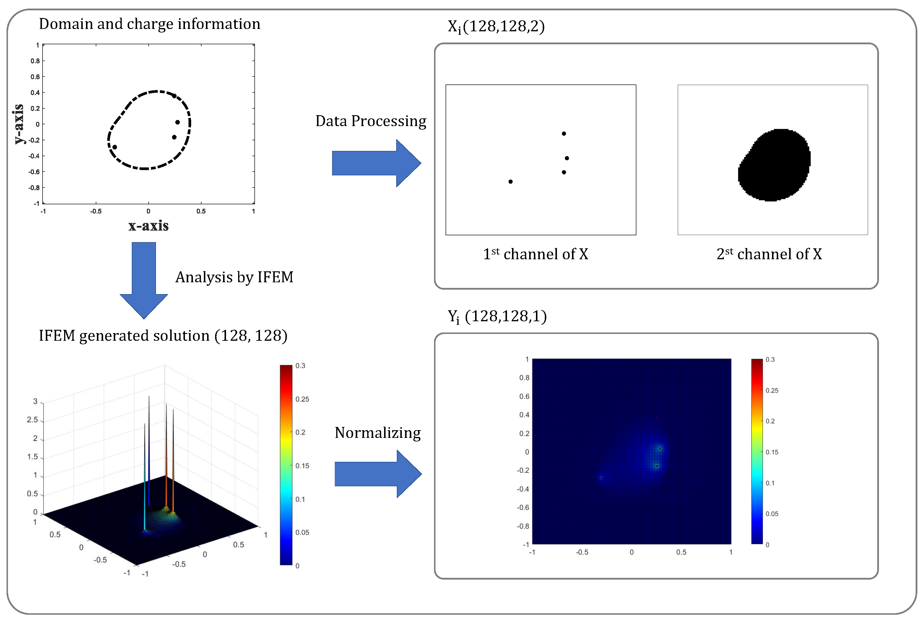
2.3. Formatting of Datasets and Data Preprocessing

In this subsection, we describe the generation process of the datasets which will be used to train neural networks. One of our goals is to develop a robust neural network regardless of the interface shapes and locations of charges. Thus, we generate various interface shapes and different locations of charges. Figure 1 shows some typical examples of such interface/charge locations. Once u h is obtained via Algorithm 1, we regularize the solutions as below since u h blows-up at the charge locations:
u h ( x ) = L , if x is the charge location , u h ( x ) = u h ( x ) , otherwise ,
where L is some fixed number to replace values. In this work, we set L = 3 .
We construct datasets in the form of ( X i , Y i ) ’s, ( i = 1 , , n S a m p l e s ) which will be used to train neural network. Figure 2 shows the summarized process of generating typical samples ( X i , Y i ) . The variable X i ’s are three-dimensional data of size ( n , n , 2 ) which contain the domain/charge information and Y i ’s are three-dimensional data of size ( n , n , 1 ) which represent electro-potentials obtained by Algorithm 1. If the meshgrid T h used in Section 2.2 has m × m nodes, we will set n = m . The first channel of X i contains the location of charges; X ( k , , 1 ) = 1 if charge is located on ( k , ) -th nodes of meshgrids and X ( k , , 1 ) = 0 otherwise. The second channel of X i ’s describe the shape of the solvent–solute interface as follows
X ( k , , 1 ) = 1 , if ( k , ) - th nodes are located in Ω , X ( k , , 1 ) = 0 , Otherwise .
For Y i , the point-wise values of u h on the nodal points of T h are subtracted to Y i , i.e., Y i ( k , ) = u h ( x k , y ) . Finally, we normalize the Y i as below so that the Y i ’s values lie between [ 0 , 1 ] :
Y i = Y i m i n m a x m i n .
Here, m a x and m i n are global maximum and minimum of the Y i before normalization which values are 3 and 0 respectively.

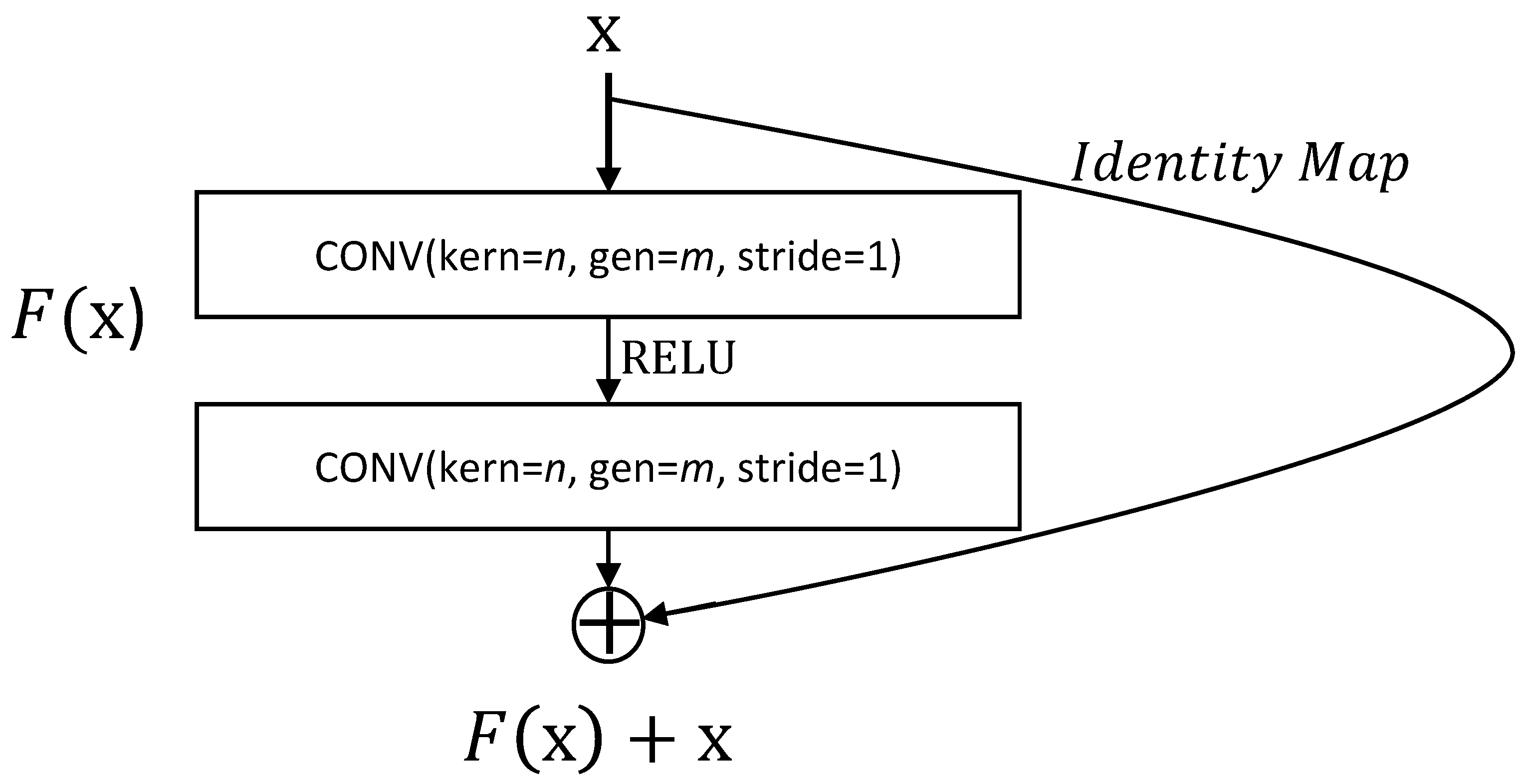
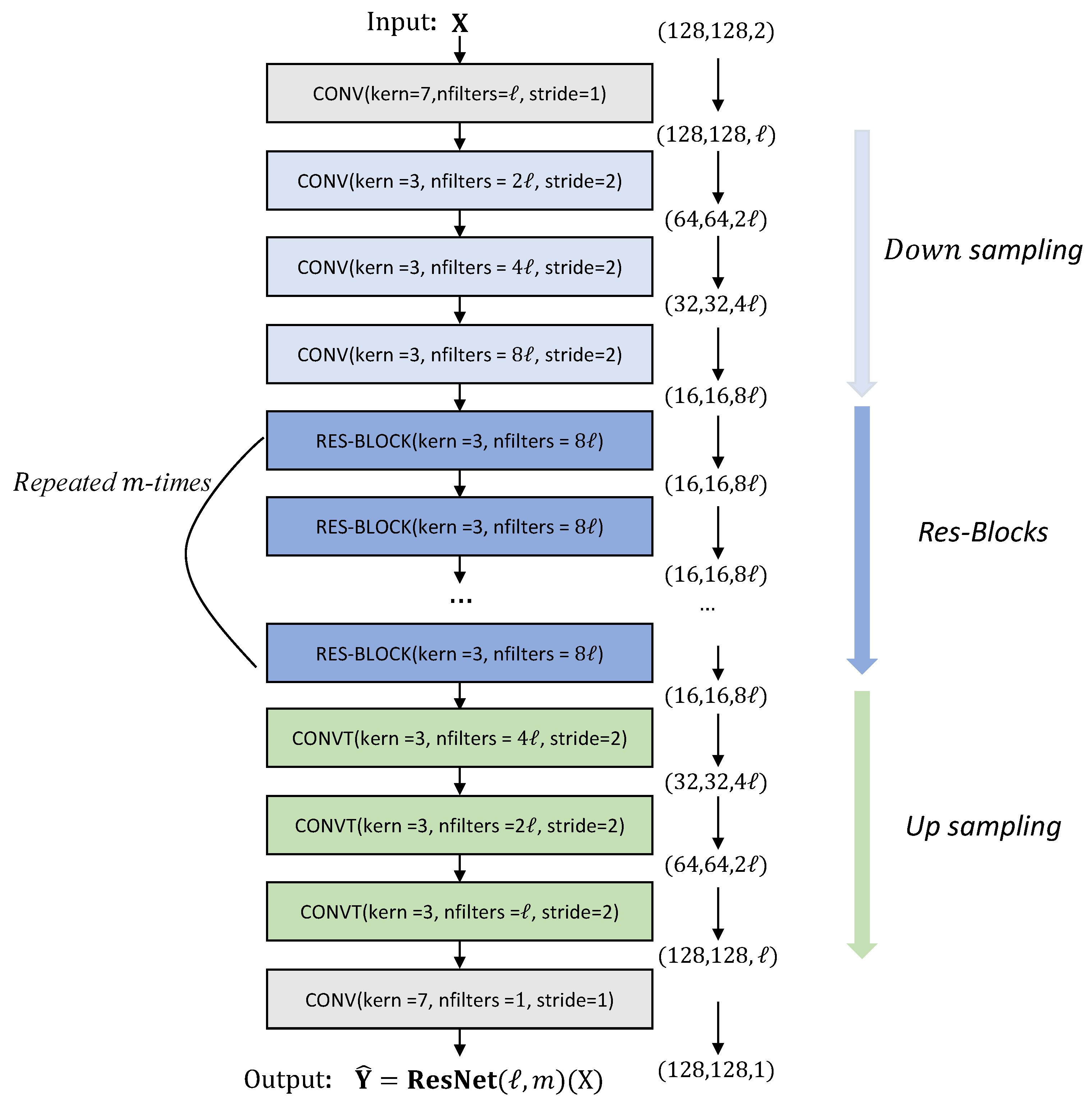
2.4. ResNet Based Artificial Neural Network for Poisson–Boltzmann Equation

In this subsection, we propose an ANN that predicts electro-potential solutions of PBE. In order to create an ANN that is robust to various combinations of charge and interface positions, we shall need a deep network with a large number of parameters. However, it is known that the so-called "gradient-vanishing" phenomenon occurs in deep neural networks without some proper care. This is because as the number of hidden layers increases, the correction terms transferred via the back-propagations tend to vanish. One of the works suggested to overcome the difficulty was proposed by He et al. [17], in which the ResNet was introduced. In [17], the concept of skip-connection is introduced, whose role is to ensure the correction term is transferred to the front layers without vanishing in the back-propagation process.
Let us introduce our version of ResNet for the solutions of PBE equations following the way of [17]. First, the concept of Res-Blocks shall be needed which plays an important role in ResNet. Let us denote convolution mapping with n by n kernel with m-number of filters as C O N V ( k e r n = n , g e n = m , s t r i d e = 1 ) . One residual block is described as
Y = F ( X ; W ) + X .
Here, F ( X ; W ) = ( C O N V · σ · C O N V ) ( X ) where σ is a RELU activation function. In particular, we denote the residual block as RES-BLOCK ( k e r n = n , g e n = m ) (Figure 3).
We are in a position to define our version of ResNet, ResNet( , m ) , whose brief illustration is given in Figure 4. First, we apply a convolutional layer with number of filters. Next, the samples are downsized with a convolutional layer with s t r i d e s = 2 but with increasing filter numbers. Then, residual blocks are applied repeatedly m times. Then, the sizes of the resulting filter maps are upsized via a transposed convolutional layer with s t r i d e s = 2 . Finally, the output is obtained by applying a sigmoid function.
To train ResNet( , m ) which can predicts solutions of PBE, we define a least square type objective function was employed as below
O b j ( θ ) = 1 n i = 1 n ( Y i Y ^ i ) 2 ,
where Y are IFEM-generated solutions and Y ^ are ResNet-generated solutions. The ADAM optimizer was used [40] to train the networks.

3. Results

We consider a domain Ω = [ 1 , 1 ] 2 and we consider a uniform triangulation T h constructed by right triangles whose size h = 2 6 , resulting in 128 × 128 nodes. Additionally, we consider an interface which is a sine-type perturbed circle,
r = r 0 ( 1 + a 0 sin ( θ θ 0 ) + a 1 sin ( 2 ( θ θ 1 ) ) + a 2 sin ( 3 ( θ θ 2 ) )
Here, a sign of r determines the subdomain, i.e. when r < 0 it means solute domain; when r > 0 it means solvent domain. The parameters are chosen as in [9,41] whose values are
ϵ 2 , ϵ + 80 , κ 2 8.847 .
We generate the 12,000 number of PBE samples via Algorithm 1. To generate samples, we used intel CPU Core(TM) i9-10940X. Here, 1000 samples were assigned in 12 CPUs (in a parallel way), thus using multiple CPUs at the same time we have generated datasets within 21,584 seconds. First, 8000 samples were assigned as train sets, next, 1000 samples were assigned as the validation set, the remaining 3000 samples were assigned as test samples. For all tests, the learning rate of the ADAM optimizer was set to 10 4 and the epoch number was set to 200.
In order to find suitable parameters in the ResNet( , m ) , we conducted various experiments with various combination of ( , m ) . The number of total layers, kernels, and neurons for each case are summarized in Table 1. Additionally, the change of data structure as input X passes through the CONV and RES-BLOCK layers is described in Figure 4. Here, all training and evaluation of the networks were conducted on a single NVIDIA RTX 3090 GPU. The results are reported in Table 2 in terms of the CPU time taken to train the network and the evaluation of networks on the test sets. For the evaluation, the usual root mean squared error (RMSE) and mean absolute error (MAE) were used whose definitions are
RMSE = 1 n i = 1 n | Y i Y ^ i | 2 , MAE = 1 n i = 1 n | Y i Y ^ i | .
One observes that as the numbers and m increase, both the number of parameters and CPU time increase. However, among various networks in Table 1, ResNet(64, 10) has the lowest errors, whose evolutions of the RMSE and MAE as increasing epochs are described at Figure 5. For all tests, RMSEs are below 5 · 10 7 and MAEs are below 3.3 · 10 4 showing that the ResNet-generated solutions converge to Algorithm 1-generated solutions via the training process of the neural network. One observes that both RMSE and MAE decrease as epochs increase for both the train set and validation set. However, we see that RMSE and MAE decrease in small amounts after epoch number>190, which is the reason why the target epoch number was set to 200.
Let us compare the shapes of ResNet-generated solutions and IFEM-generated solutions in Figure 6 where first column contains the information of domain/charge information, second and third columns contain the ResNet ( Y ^ i ) and IFEM-solutions ( Y i ) respectively, and fourth column shows the difference between solutions ( | Y i Y ^ i | ). We see that both Y i and Y i reflect the effects of the singular charges, i.e., the electro-potential blowups near the charges. Additionally, the phenomena of abrupt decreases of potential near the solute–solvent interfaces are described well by ResNet. Thus, we may conclude that ResNet represents the effects of charges and interfaces on the electro-potentials. As for the differences between solutions, max | Y i Y ^ i | are below 0.01 for all cases, which is only 0.33 % compared to the maximum of IFEM solutions. On the other hand, we see that the errors tend to be large near the locations of charges. This issue might be handled in future works.

4. Discussion and Conclusions

Predicting solutions of PBE can be used effectively in many disciplinaries including biophysics, electrochemistry, and colloid chemistry [1,2,3,4,5,6]. However, FEM/FDM-based numerical methods developed so far are rather complicated to implement which makes the real-time simulation of PBE solutions almost impossible. In this study, we develop a ResNet-based ANN to predict solutions of PBE, which we name ResNet ( , m ) where and m are parameters determining the depth and complexity of the network. One of the main advantages of our algorithms is that one can predict solutions of PBE in almost real time once the networks are trained. Additionally, our networks are robust with respect to the locations of charges and interfaces. Thus, our model can be used effectively in various biomolecular simulations including ion-channeling simulations [13] and calculations of diffusion-controlled enzyme reaction rate [32]. To generate train and test sets, we have solved PBE using Algorithm 1 proposed in [9]. The results show that RMSE errors between ResNet generated solutions and IFEM generated solutions are below 5 · 10 7 ; thus one may conclude that ResNet are trained enough. Additionally, blow-ups of electrostatic potentials near the singular charge and abrupt decreases near the interfaces are represented reasonably by the predictions of ResNet. Therefore, we have proposed a convenient and efficient way of predicting solutions of PBE by substituting the charge/interface information to ResNet. On the other hand, the differences of ResNet-solutions and IFEM-solutions are found to be relatively high near the charges. The issue of reducing or smoothing the errors near the charges is left as future work. Additionally, we will extend our results in three-dimensional cases. Finally, let us discuss the possible applications of the proposed ResNet. First, our methods can be used effectively in simulations of biological processes based on ion-channeling such as ionic movements through transmembrane channels. Moreover, we can employ our methods in the study of diffusion-controlled enzyme reactions such as analysis of the effects of the substrate–enzyme interactions on the concentration variation of biomolecules or reagents [32].

Author Contributions

Conceptualization, G.J. and I.K.; methodology, K.-S.S. and I.K.; writing—original draft preparation G.J. and I.K.; supervision, G.J. and K.-S.S. All authors have read and agreed to the published version of the manuscript.

Funding

The second author is supported by the National Research Foundation of Korea (NRF) grant funded by the Korean government (MSIT) (No. 2020R1C1C1A01005396). The third author is supported by the NRF grant funded by MSIT (No. NRF-2019R1G1A1087290).

Institutional Review Board Statement

Not applicable.

Informed Consent Statement

Not applicable.

Data Availability Statement

The data presented in this study are available on request from the corresponding author.

Conflicts of Interest

The authors declare no conflict of interest.

References

  1. Guoy, G. Constitution of the electric charge at the surface of an electrolyte. J. Phys. 1910, 9, 457–467. [Google Scholar]
  2. Chapman, D.L. A contribution to the theory of electrocapillarity. Lond. Edinb. Dublin Philos. Mag. J. Sci. 1913, 25, 475–481. [Google Scholar] [CrossRef] [Green Version]
  3. Derjaguin, B.; Landau, L. Theory of the stability of strongly charged lyophobic sols and the adhesion of strongly charged particles in solutions of electrolytes. Prog. Surf. Sci. 1993, 43, 30–59. [Google Scholar] [CrossRef]
  4. Verwey, E.J.W.; Overbeek, J.T.G.; Van Nes, K. Theory of the Stability of Lyophobic Colloids: The Interaction of Sol Particles having an Electric Double Layer; Elsevier Publishing Company: Amsterdam, The Netherlands, 1948. [Google Scholar]
  5. Davis, M.E.; McCammon, J.A. Electrostatics in biomolecular structure and dynamics. Chem. Rev. 1990, 90, 509–521. [Google Scholar] [CrossRef]
  6. Honig, B.; Nicholls, A. Classical electrostatics in biology and chemistry. Science 1995, 268, 1144–1149. [Google Scholar] [CrossRef] [PubMed] [Green Version]
  7. Chern, I.L.; Liu, J.G.; Wang, W.C. Accurate evaluation of electrostatics for macromolecules in solution. Methods Appl. Anal. 2003, 10, 309–328. [Google Scholar] [CrossRef]
  8. Chen, L.; Holst, M.J.; Xu, J. The finite element approximation of the nonlinear Poisson–Boltzmann equation. SIAM J. Numer. Anal. 2007, 45, 2298–2320. [Google Scholar] [CrossRef]
  9. Kwon, I.; Kwak, D.Y. Discontinuous bubble immersed finite element method for Poisson-Boltzmann equation. Commun. Comput. Phys. 2019, 25, 928–946. [Google Scholar] [CrossRef]
  10. Borleske, G.; Zhou, Y.C. Enriched gradient recovery for interface solutions of the Poisson-Boltzmann equation. J. Comput. Phys. 2020, 421, 109725. [Google Scholar] [CrossRef]
  11. Ramm, V.; Chaudhry, J.H.; Cooper, C.D. Efficient mesh refinement for the Poisson-Boltzmann equation with boundary elements. J. Comput. Chem. 2021, 42, 855–869. [Google Scholar] [CrossRef] [PubMed]
  12. Wang, S.; Alexov, E.; Zhao, S. On regularization of charge singularities in solving the Poisson-Boltzmann equation with a smooth solute-solvent boundary. Math. Biosci. Eng. 2021, 18, 1370–1405. [Google Scholar] [CrossRef] [PubMed]
  13. Kwon, I.; Kwak, D.Y.; Jo, G. Discontinuous bubble immersed finite element method for Poisson-Boltzmann-Nerst-Plank model. J. Comput. Phys. 2021, 438, 110370. [Google Scholar] [CrossRef]
  14. Shestakov, A.I.; Milovich, J.L.; Noy, A. Solution of the nonlinear Poisson-Boltzmann equation using pseudo-transient continuation and the finite element method. J. Colloid Interface Sci. 2002, 247, 62–79. [Google Scholar] [CrossRef]
  15. Lo, S.C.B.; Chan, H.P.; Lin, J.S.; Li, H.; Freedman, M.T.; Mun, S.K. Artificial convolution neural network for medical image pattern recognition. Neural Netw. 1995, 8, 1201–1214. [Google Scholar] [CrossRef]
  16. Szegedy, C.; Ioffe, S.; Vanhoucke, V.; Elemi, A.A. Inception-v4, inception-resnet and the impact of residual connections on learning. In Proceedings of the Thirty-First AAAI Conference on Artificial Intelligence, San Francisco, CA, USA, 4–9 February 2017. [Google Scholar]
  17. He, K.; Zhang, X.; Ren, S.; Sun, J. Deep residual learning for image recognition. In Proceedings of the IEEE Conference on Computer Vision and Pattern Recognition, Las Vegas, NV, USA, 27–30 June 2016; pp. 770–778. [Google Scholar]
  18. Devlin, J.; Chang, M.-W.; Lee, K.; Toutanova, K. Bert: Pre-training of deep bidirectional transformers for language understanding. arXiv 2018, arXiv:1810.04805. [Google Scholar]
  19. Brown, T.B.; Mann, B.; Ryder, N.; Subbiah, M.; Kaplan, J.; Dhariwal, P.; Neelakantan, A.; Shyam, P.; Sastry, G.; Askell, A.; et al. Language models are few-shot learners. arXiv 2020, arXiv:2005.14165. [Google Scholar]
  20. Deng, L.; Liu, Y. Deep Learning in Natural Language Processing; Springer: Berlin/Heidelberg, Germany, 2018. [Google Scholar]
  21. Purwins, H.; Li, B.; Virtanen, T.; Schlüter, J.; Chang, S.-Y.; Sainath, T. Deep learning for audio signal processing. IEEE J. Sel. Top. Signal Process. 2019, 13, 206–219. [Google Scholar] [CrossRef] [Green Version]
  22. Yu, D.; Deng, L. Deep learning and its applications to signal and information processing. IEEE Signal Process. Mag. 2010, 28, 145–154. [Google Scholar]
  23. Ngiam, J.; Khosla, A.; Kim, M.; Nam, J.; Lee, H.; Andrew, Y.N. Multimodal deep learning. ICML 2011. [Google Scholar]
  24. Tang, W.; Shan, T.; Dang, X.; Li, M.; Yang, F.; Xu, S.; Wu, J. Study on a Poisson’s equation solver based on deep learning technique. In Proceedings of the 2017 IEEE Electrical Design of Advanced Packaging and Systems Symposium, Haining, China, 14–16 December 2017. [Google Scholar]
  25. Antil, H.; Di, Z.W.; Khatri, R. Bilevel optimization, deep learning and fractional Laplacian regularization with applications in tomography. Inverse Probl. 2020, 36, 064001. [Google Scholar] [CrossRef] [Green Version]
  26. Chen, R.T.Q.; Rubanova, Y.; Bettencourt, J.; Duvenaud, D. Neural ordinary differential equations. arXiv 2018, arXiv:1806.07366. [Google Scholar]
  27. Ruthotto, L.; Haber, E. Deep neural networks motivated by partial differential equations. J. Math. Imaging Vis. 2020, 62, 352–364. [Google Scholar] [CrossRef] [Green Version]
  28. Kim, M.; Winovich, N.; Lin, G.; Jeong, W. Peri-Net: Analysis of Crack Patterns Using Deep Neural Networks. J. Peridynamics Nonlocal Model. 2019, 1, 131–142. [Google Scholar] [CrossRef] [Green Version]
  29. Haghighat, E.; Bekar, A.C.; Madenci, E.; Juanes, R. A nonlocal physics-informed deep learning framework using the peridynamic differential operator. Comput. Methods Appl. Mech. Eng. 2021, 385, 114012. [Google Scholar] [CrossRef]
  30. Kutz, J.N. Deep learning in fluid dynamics. J. Fluid Mech. 2017, 814, 1–4. [Google Scholar] [CrossRef] [Green Version]
  31. Liu, B.; Tang, J.; Huanga, H.; Lu, X.Y. Deep learning methods for super-resolution reconstruction of turbulent flows. Phys. Fluids 2020, 32, 025105. [Google Scholar] [CrossRef]
  32. Lu, B.; Zhou, Y.C.; Huber, G.A.; Bond, S.D.; Holst, M.J.; McCammon, J.A. Electrodiffusion: A continuum modeling framework for biomolecular systems with realistic spatiotemporal resolution. J. Chem. Phys. 2007, 127, 10B604. [Google Scholar] [CrossRef]
  33. Kwak, D.Y.; Jin, S.; Kyeong, D. A stabilized P1-nonconforming immersed finite element method for the interface elasticity problems. Esaim Math. Model. Numer. Anal. 2017, 51, 187–207. [Google Scholar] [CrossRef]
  34. Jo, G.; Kwak, D.Y. An IMPES scheme for a two-phase flow in heterogeneous porous media using a structured grid. Comput. Methods Appl. Mech. Eng. 2017, 317, 684–701. [Google Scholar] [CrossRef] [Green Version]
  35. Jo, G.; Kwak, D.Y. Recent development of immersed fem for elliptic and elastic interface problems. J. Korean Soc. Ind. Appl. Math. 2019, 23, 65–92. [Google Scholar]
  36. Jo, G.; Kwak, D.Y. A Reduced Crouzeix–Raviart Immersed Finite Element Method for Elasticity Problems with Interfaces. Comput. Methods Appl. Math. 2020, 20, 501–516. [Google Scholar] [CrossRef]
  37. Jo, G.; Kwak, D.Y.; Lee, Y.-J. Locally Conservative Immersed Finite Element Method for Elliptic Interface Problems. J. Sci. Comput. 2021, 87, 1–27. [Google Scholar] [CrossRef]
  38. Feng, W.; He, X.; Lin, Y.; Zhang, X. Immersed finite element method for interface problems with algebraic multigrid solver. Commun. Comput. Phys. 2014, 15, 1045–1067. [Google Scholar] [CrossRef]
  39. Jo, G.; Kwak, D.Y. Geometric multigrid algorithms for elliptic interface problems using structured grids. Numer. Algorithms 2019, 81, 211–235. [Google Scholar] [CrossRef]
  40. Kingma, D. P; Ba, J. Adam: A method for stochastic optimization. arXiv 2014, arXiv:1412.6980. [Google Scholar]
  41. Holst, M.J. Multilevel Methods for the Poisson-Boltzmann Equation. Ph.D. Thesis, Universitiy of Illinois at Urbana, Champaign, IL, USA, 1993. [Google Scholar]
Figure 1. Typical examples of interface/charge locations. The dashed line shows the interface ( Γ ) between solvent domain ( Ω + ) and molecular domain ( Ω ). Black dots inside Ω indicates the locations of the charges.
Electronics 10 02627 g001
Figure 2. Illustration of typical sample ( X i , Y i ) generation. Input sample X i consists of two channels; first channel shows the location of charge source and second channel shows the shape of the subdomains separated by interface Γ . Output sample is given by the IFEM-simulated PB solution.
Electronics 10 02627 g002
Figure 3. Description of RES-BLOCK ( k e r n = n , g e n = m ) .
Electronics 10 02627 g003
Figure 4. Architecture of ResNet ( k e r n = , g e n = n ) .
Electronics 10 02627 g004
Figure 5. Evolution of objective function and MAE accuracy as epoch number increases.
Electronics 10 02627 g005
Figure 6. Comparison of ResNet generated solution Y ^ and IFEM-solutoin Y.
Electronics 10 02627 g006
Table 1. The number of total layers, kernels, neurons appearing in ResNet ( , m ) as and m change. A size of input ( X ) is ( 128 , 128 , 2 ) and a size of output ( Y ^ ) is ( 128 , 128 , 1 ) for each network.
ResNet( , m )# Layers# Kernels# Parameters
(16, 10)2829133,147,921
(16, 20)4854736,099,601
(32, 10)28582512,581,153
(32, 20)4810,94524,382,753
(64, 10)2811,64950,303,553
(64, 20)4821,88997,499,713
Table 2. Performance of ResNet( , m ) with various combinations of ( , m ) in terms of total number of parameters, CPU time, RMSE, and MAE.
ResNet( , m )# ParametersCPU time (s)RMSEMAE
(16, 10)3,147,92120904.71 × 10−72.25 × 10⁻⁴
(16, 20)6,099,60128764.87 × 10−72.20 × 10⁻⁴
(32, 10)12,581,15337793.85 × 10−72.20 × 10⁻⁴
(32, 20)24,382,75355693.66 × 10−72.01 × 10⁻⁴
(64, 10)50,303,55385653.45 × 10−72.13 × 10⁻⁴
(64, 20)97,499,71313,2643.81 × 10−72.07 × 10⁻⁴
Publisher’s Note: MDPI stays neutral with regard to jurisdictional claims in published maps and institutional affiliations.

