Article

Modeling and Control of a Phase-Shifted Full-Bridge Converter for a LiFePO4 Battery Charger

by
Ivan A. Mendoza-Varela
,
Alfredo Alvarez-Diazcomas
,
Juvenal Rodriguez-Resendiz
and
Miguel Angel Martinez-Prado
*
Faculty of Engineering, Autonomous University of Queretaro, Queretaro 76010, Mexico
*
Author to whom correspondence should be addressed.
Electronics 2021, 10(21), 2568; https://doi.org/10.3390/electronics10212568
Submission received: 17 September 2021 / Revised: 9 October 2021 / Accepted: 15 October 2021 / Published: 21 October 2021

Abstract

:
A proper charge in an electric vehicle (EV) battery allows it to have a longer useful life and lower maintenance costs. For this purpose, the voltage and current supplied to the battery must be precisely regulated. In this article, the model of a phase-shifted full-bridge (PSFB) converter is obtained. Moreover, a dual control loop was designed to regulate the state of charge of a lithium ferrofosfate (LiFePO 4 ) battery. The autoregressive exogenous (ARX) model is used to model the system. Once the plant model is obtained, it is controlled using a classical controller. A couple of cases are evaluated where the control parameters are modified, and the best approach is selected. From the obtained model, the controller is designed for the proposed cases. The theoretical controller response is compared with the experimental response. The results show a 94% accuracy of the model. In the same way, the result obtained from the controller is accurate in a 96% by comparing it with a simulation. Both the modeling and the control obtained experimentally resemble the results obtained theoretically. The controller manages to respond as expected in all proposed cases.

1. Introduction

Currently, environmental care is of great relevance for humankind. Several alternatives have been developed in the face of those factors that lead to its deterioration. EVs are an alternative to pollution generated by the transport sector and are beginning to become more popular [1]. This sector is responsible for up to 29% of the energy consumed worldwide and up to 65% of oil consumption [2].
As energy source, EVs use lithium-ion batteries, mainly due to their high energy density. It is essential to properly charge the battery so that it can fulfill its useful life. The state of charge of a battery will depend on the material from which it is made. Lithium batteries offer a higher voltage and energy density compared to batteries of different materials [3]. It also has good structural and chemical stability, allowing the battery to have more charge cycles and a longer lifetime.
There has been a dramatic increase in research and commercialization of lithium-ion batteries for energy storage in EVs and plug-in hybrid electric vehicles (PHEVs) in recent years. Challenges remain in manufacturing low-cost, high-performance, and high-safety lithium-ion batteries for vehicle applications.
The most common materials for EV batteries are lithium–nickel–cobalt–aluminum (NCA), lithium–cobalt oxide (LiCoO 2 ), lithium–nickel–manganese–cobalt (LiNMC), lithium–manganese oxide (LMO), lithium titanate (LTO), and lithium ferrophosphate (LiFePO 4 ). Each material has different characteristics, so it is difficult to select the best battery, since each technology has its advantages and disadvantages. However, LiFePO 4 batteries have started to become popular mainly because of their low cost and long lifespan [4].
Different studies of topologies used for EV charging, conversion stages, and power levels have been presented [5,6,7,8] as well as projects to obtain a higher efficiency from batteries [9]. These studies have made it possible to clarify the topologies that can be useful for battery charging and the advantages and disadvantages of each one. Furthermore, topologies of full-bridge isolated converters have been proposed [10,11,12]. In these architectures, the efficiency increases, and the cost is reduced using a proper switching strategy.
From this research, various EV battery charger designs have been made. A high efficient non-isolated single-stage on-board battery charger (OBC) has been designed and implemented for EV [13]. A detailed theoretical analysis, operational strategy, and experimental results have been presented.
An isolated Level 2 OBC has also been introduced using silicon carbide (SiC) power devices to achieve high density and high efficiency for application in EV and PHEV. This charger has a two-stage architecture in which the first stage is a bridgeless AC-DC converter, and the second stage is a PSFB isolated DC-DC converter. The operation of both topologies is presented, and the specific advantages obtained by using SiC power devices are discussed [14]. Similarly, studies have been introduced where harmonic distortion and switching losses in converters are studied. Such is the case of [15], where a new bidirectional buck-boost three-phase DC-AC topology is presented, where it is possible to reduce both the harmonic distortion in the mains currents and the switching losses.
The design of a controller for a converter can vary widely depending on the electrical needs and the load. In [16], a model predictive control is proposed to control the power flow between the high voltage and low voltage DC buses of a bidirectional isolated full-bridge DC-DC converter. For this article, a classical controller is proposed, which is enough for this application.
To properly charge the battery, it is necessary to regulate both the voltage and the current supplied. The most used charging algorithms for batteries focus on having a constant voltage, constant current, and trickle charge [17].
This article analyzes the procedure to obtain the modeling of the PSFB converter to obtain the transfer function of the converter and perform a constant voltage control. The results show that the model presents an accuracy of 94%. Moreover, the result obtained from the controller is accurate in a 96% by comparing it with a simulation.
In Section 2, the operating principle of the selected converter is discussed. Section 3 describes the methodology used in this work. Finally, in Section 4, the conclusions are presented.

2. Theoretical Background

This section presents, compares, and classifies the most used DC-DC converters.

2.1. DC-DC Converters
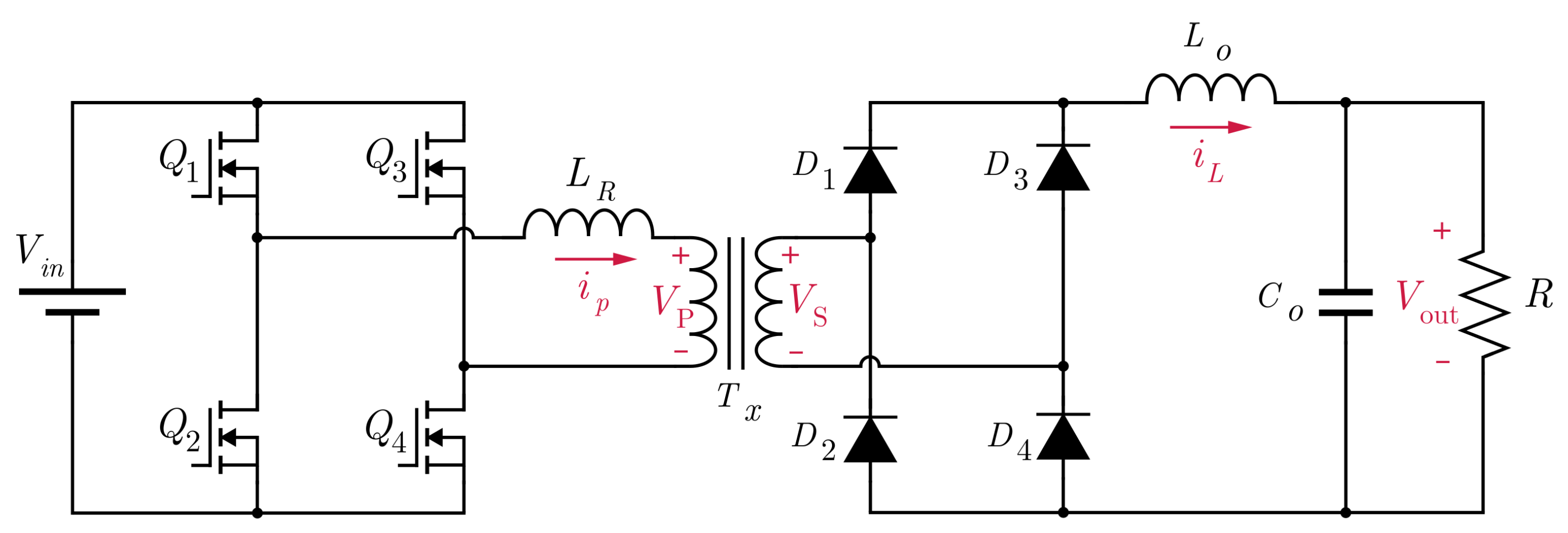
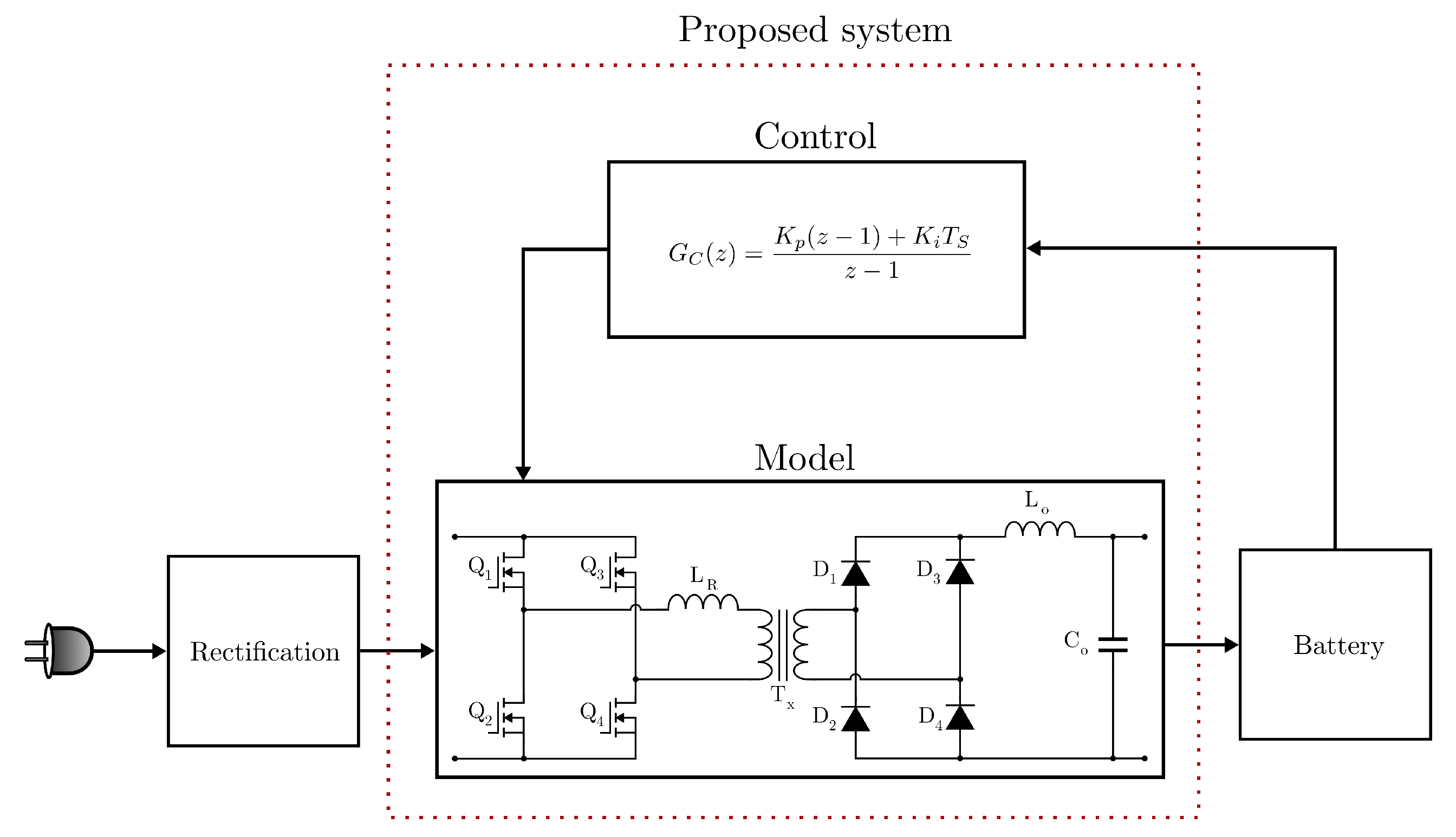
DC-DC converters have the main characteristic of operating at high frequencies and being more efficient. Metal–oxide–semiconductor field-effect transistors (MOSFETs) are most often used as switches because they can work at the required frequency as it is suggested in [18]. Working at high frequency allows the converters to be reduced in size.
Converter topologies must also be considered, as they do not all serve the same purpose. A DC-DC converter is generally responsible for converting an input voltage into an output voltage of different magnitude and sometimes of opposite polarity or with galvanic isolation between the input and output. However, there are converter topologies that, for example, raise the input voltage while others lower it. Based on the presence of galvanic isolation between input and output, DC-DC converters can be divided into two classes: non-isolated and isolated. The most common non-isolated DC-DC converters are the buck converter, the boost converter, and the single-ended primary-inductor converter (SEPIC). Isolated DC-DC converters are derived from non-isolated DC-DC converters by incorporating transformers and rectifier circuits at the output. Some articles have proposed isolated converters different from the conventional ones, improving specific electrical characteristics. Some examples of isolated converters can be found in [19,20,21], where the presented design allows a larger voltage conversion ratio compared to conventional topologies.
For the battery charging application, the isolated DC-DC converters derived from the buck converter are considered. These include the forward, push–pull, half-bridge, and full-bridge converters. Table 1 presents a comparison of the most widely used step-down DC-DC isolated converters and their parameters.
The PSFB converter can withstand a higher amount of voltage and current without increasing the size of its components since it has four switches, which help reduce the stress between them.

2.2. PSFB Converter

A PSFB shown in Figure 1 is selected for this application. The amount of phase shift between the switch control signals determines the amount of energy transferred.
This converter comprises an inverter, a transformer, a rectifier, and an output filter. The converter has an inverter because when working with alternating current, the electrical components are smaller in size compared to working with direct current. The transformer is responsible for reducing the amplitude of the AC signal. Finally, a rectifier is needed to convert the AC signal of the grid into direct current.

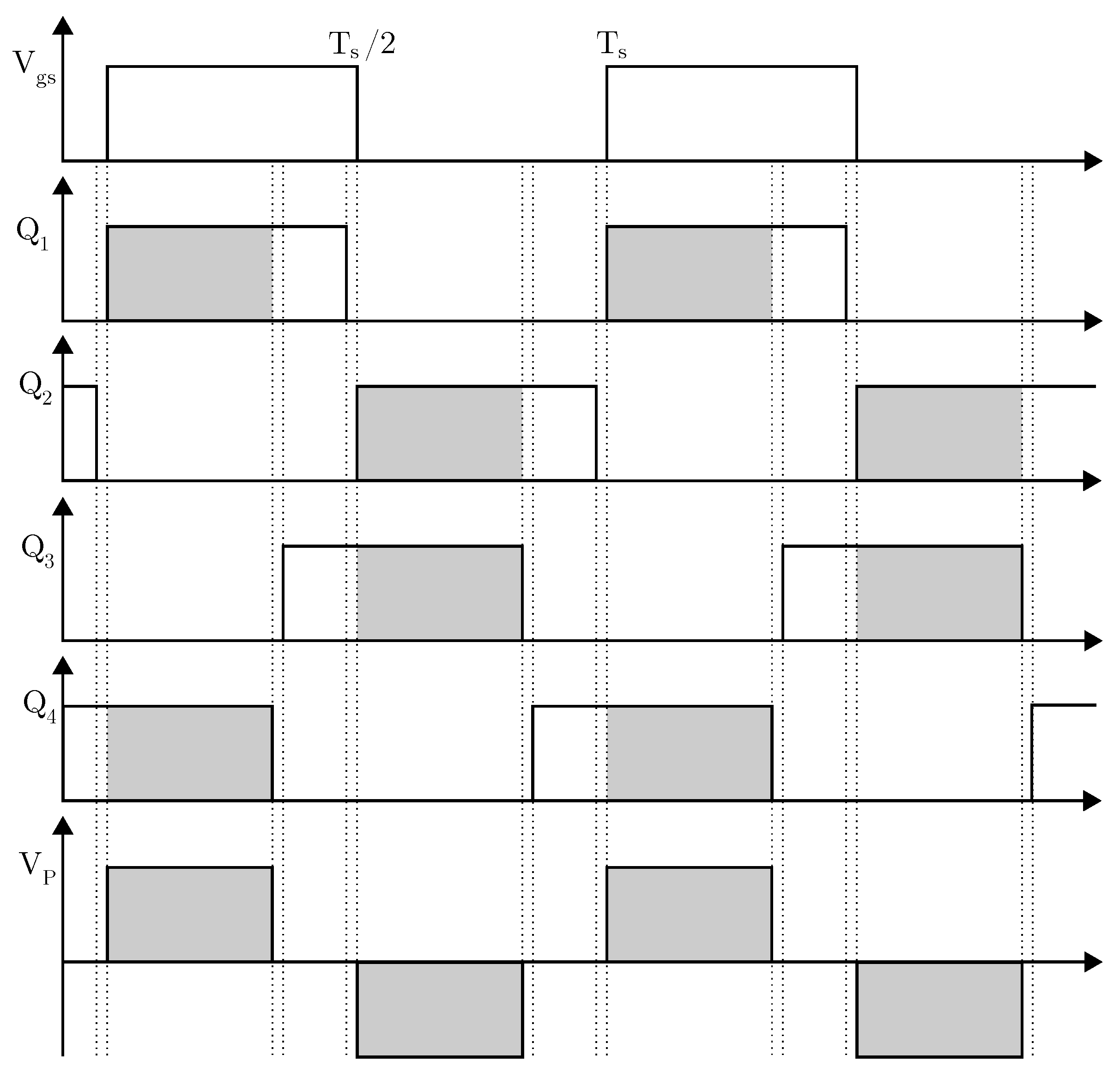
2.3. Principle of Operation
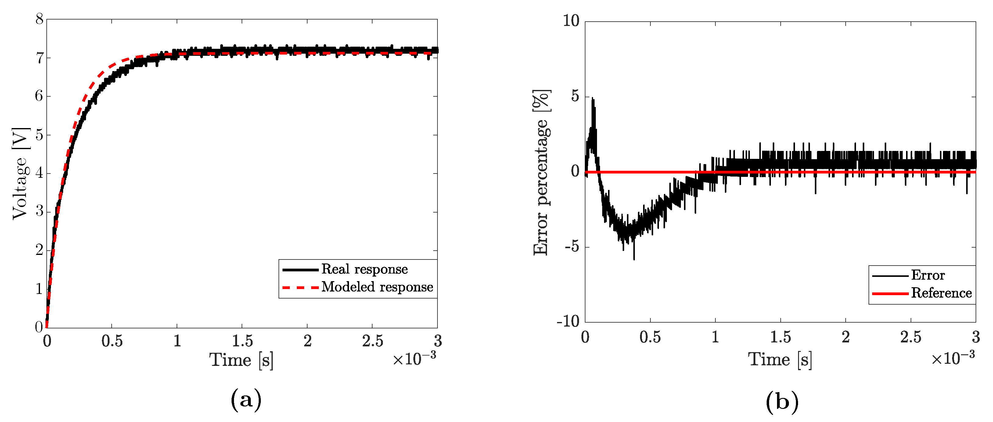
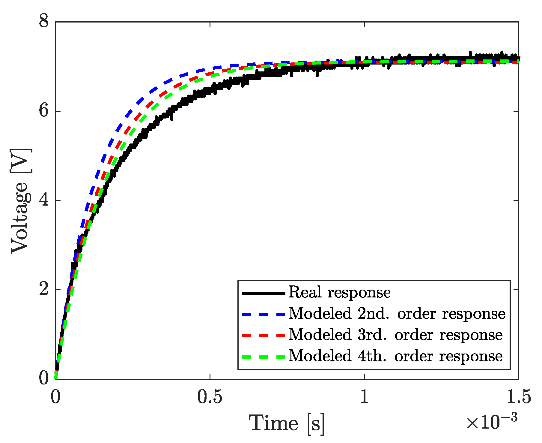
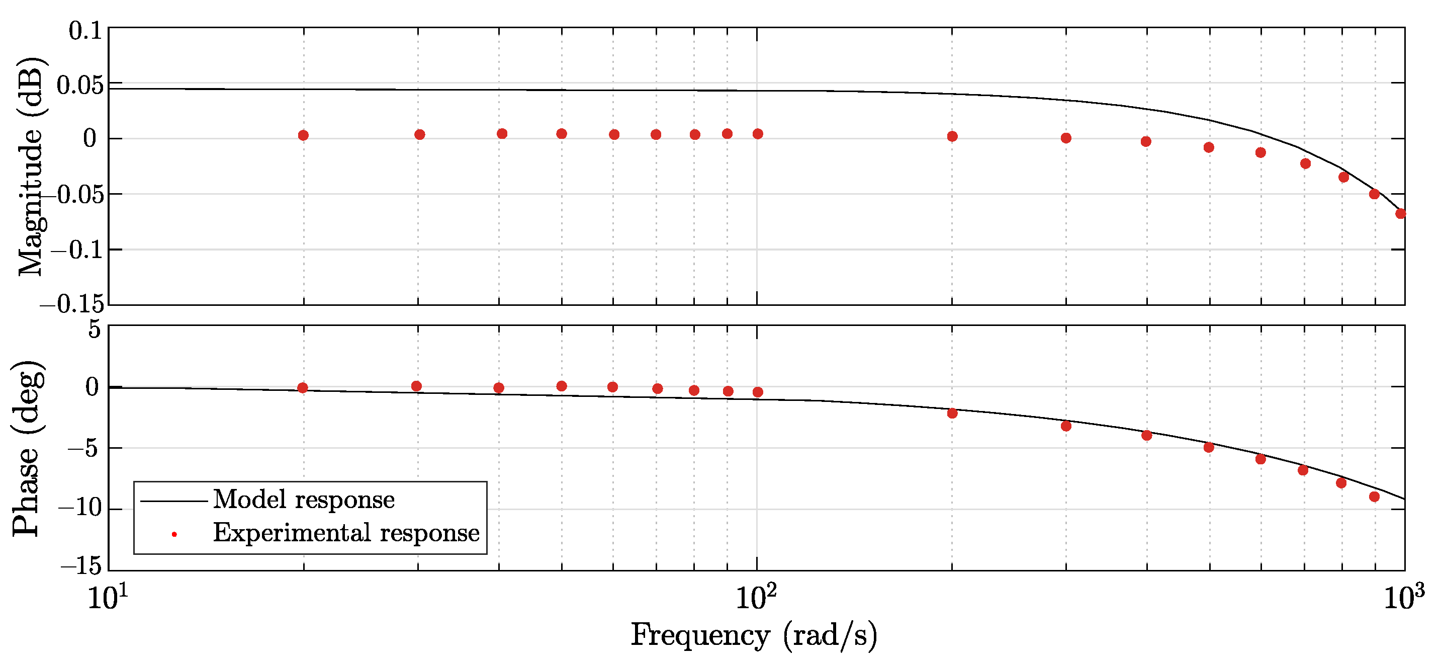
In the PSFB converter, the duty cycle is set at 50% and the power transfer is determined by the phase shift between the pair of switches Q 1 and Q 2 and the pair Q 3 and Q 4 . This explanation can be seen in Figure 2. The overlapping pairs of switches generate an AC signal. AC voltage is applied to the primary side of the transformer, allowing the MOSFETs to switch without additional circuitry. The transformer located between the full-bridge converter and the rectifier transfers the electrical energy. Finally, the voltage from the secondary winding of the transformer passes through the rectifier and the filtering section and is converted back to direct current.
The voltage applied to the output inductor L o is expressed by the following equation:
V L = n V i n V o u t
where n is the turns ratio of the transformer, V i n is the input voltage and V o u t is the output voltage.
The transfer of the converter voltage is expressed as:
V L · D T s = n ( V i n V o u t ) · D T s = V o u t T s 2 D T s
where D is the phase shift present in the PSFB converter and T s is the sampling period.

2.4. Plant Modeling

The identification of dynamic processes can be based on different models that describe several stochastic environments. Equation error models represent a beneficial category of models because of their broad applicability in prediction and control.
Some works, shown in Table 2, have used identification methods to facilitate calculations when building the mathematical model of converters.
The autoregressive exogenous (ARX) model is a way to represent a dynamic process driven by input and noise. This model describes the observed output of the process as the sum of a regression on previous input and output observations.
In this model, both the input and the output are known, but the noise in practice is unknown and can occur in various ways. Considering this element allows the analysis to be closer to reality.
The linear model of the system is written as follows:
y ( k ) = j = 1 n a j y ( k j ) + j = 0 n b j u ( k j ) + e ( k )
The noise of the model, e ( k ) , will be white noise, that is, the mean of its values will be equal to zero.
E { e ( k ) } = 0
Regarding the variance, it can be expressed as follows:
E { e 2 ( k ) } = σ 2
Since the statistical properties of e ( k ) have been defined, the model can be rewritten as:
y ( k ) = y ^ ( k ) + e ( k )
and starting from the linear model of the system, it can be observed that:
y ^ ( k ) = j = 1 n a j y ( k j ) + j = 0 n b j u ( k j )
If the Z transform is applied to these sums, they can be expressed as follows:
A ( z ) = a 1 z 1 + a 2 z 2 + + a n z n
B ( z ) = b 0 + b 1 z 1 + b 2 z 2 + + b n z n
Considering then the previous terms and the ARX model, it can be written as follows:
Y ( z ) = B ( z ) 1 A ( z ) U ( z ) + V ( z )
V ( z ) represents the white noise that is introduced at the plant output, which can be expressed as:
V ( z ) = 1 1 A ( z ) E ( z )
If the inverse Z transform is applied to Equation (11) and Equation (8) is considered, v ( k ) can be expressed as:
v ( k ) = i = 1 n a i v ( k i ) + e ( k )
For the ARX model to be implemented in recursive identification algorithms, it has to be given a different form. The summations of Equation (3) are rewritten as vectors and the parameters and measurements are separated. The parameter vector is as follows:
P T = [ b 0 , a 1 , b 1 , , a n , b n ]
and the measurement vector:
z T ( k ) = [ u ( k ) , y ( k 1 ) , u ( k 1 ) , , y ( k n ) , u ( k n ) ]
Both P T and z T ( k ) have a dimension of 1 × ( 2 n + 1 ) . These two vectors are substituted in Equation (3) to be as follows:
y ( k ) = P T z ( k ) + e ( k )
This model can be modified so that the value k is now the number of observations t with respect to the inputs and outputs. When making the change, it remains:
Y T ( t ) = P T Z T ( t ) + E T ( t )
This means that multivariable systems are considered, so Y T ( t ) is:
Y T ( t ) = [ y ( 1 ) , y ( 2 ) , , y ( t ) ]
The error has a similar change:
E T ( t ) = [ e ( 0 ) , e ( 1 ) , , e ( t ) ]
Finally, Z T ( t ) is an array of dimension ( 2 n + 1 ) × t and looks like this:
Z T ( t ) = u ( 1 ) u ( 2 ) u ( t ) y ( 0 ) y ( 1 ) y ( t 1 ) u ( 0 ) u ( 1 ) u ( t 1 ) y ( 1 n ) y ( 2 n ) y ( t n ) u ( 1 n ) u ( 2 n ) u ( t n )
With this form of the ARX model, it can begin to be implemented in a recursive identification algorithm.

2.5. Least Squares Method for Estimating Parameters of the ARX Model
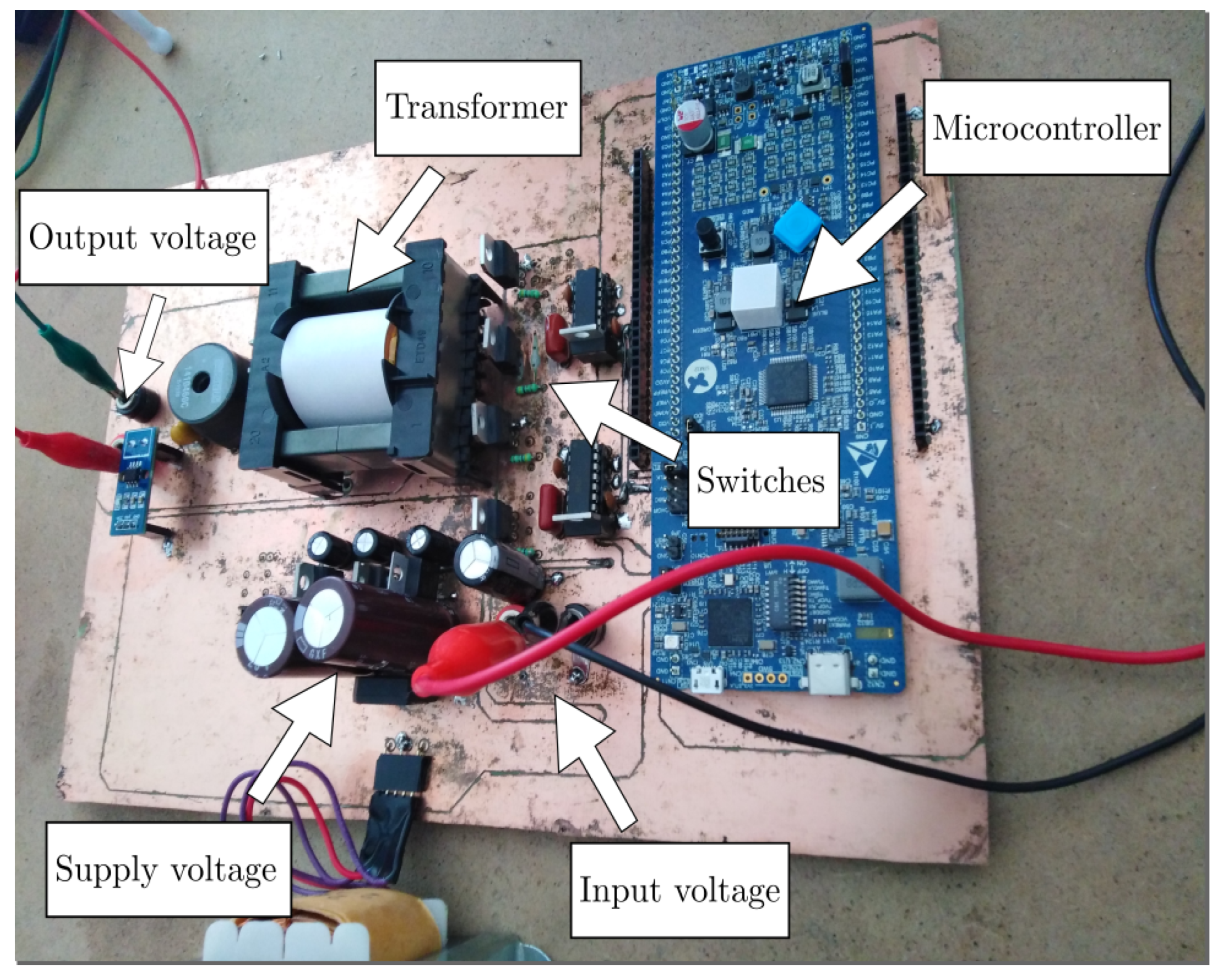
As seen in the structure of the ARX model, there is a disturbance in the form of white noise, so the output Y T ( t ) in Equation (16) has statistical properties like the error where the mean of the output is:
E { Y T ( t ) } = P T Z T ( t )
and the covariance of the output is:
c o v { Y ( t ) } = c o v { E ( t ) } = σ 2 I
where I is defined by the identity matrix.
Now it is necessary to minimize the quadratic form depending on the estimation of the parameters contained in P. This is done with the method of least squares.
J = ( Y ( t ) Z ( t ) P ( t ) ) T W ( Y ( t ) Z ( t ) P ( t ) )
In this equation, W is called a weight matrix. This matrix can be defined in different ways, however, for this case, W = I is considered. With this consideration, Equation (22) remains as:
J = Y T ( t ) Y ( t ) 2 Y T ( t ) Z ( t ) P ( t ) + P T ( t ) Z T ( t ) Z ( t ) P ( t )
It is derived with respect to P ( t ) to find the least squares estimator and thus apply the least squares method. The derivative is:
J P ( t ) = 2 Z T ( t ) Y ( t ) + 2 Z T ( t ) Z ( t ) P ( t ) = 0
Solving for the least squares estimator:
P ^ T ( t ) = ( Z T ( t ) Z ( t ) ) 1 Z T ( t ) Y ( t )

3. Methodology

The first step is to obtain the samples from the test bench in order to to apply the method previously described. The test bench is shown in Figure 3 and is conformed by the components shown in Table 3.

3.1. Converter Efficiency

In this section, the computation of the losses of the components is done to determine the efficiency of the converter.

3.1.1. Transformer

The secondary current is obtained by the following equation:
I S = I S 1 2 + I S 2 2 + I S 3 2 = 1 . 2 2 + 0 . 55 2 + 0 . 2 2 = 1.31 [ A ]
where:
I S 1 = Secondary current when energy delivered to secondary;
I S 2 = Secondary current when diode pair is conducting;
I S 3 = Secondary current caused during freewheeling period.
The primary current is obtained by the following equation:
I P = I P 1 2 + I P 2 2 = 0 . 7 2 + 0 . 4 2 = 0.81 [ A ]
where:
I P 1 = Primary current when energy delivered to secondary;
I P 2 = Primary current caused during freewheeling period.
The estimated transformer losses are obtained considering copper losses and core losses.
P T I P 2 × D C R P + I S 2 × D C R S + P c o r e 0 . 81 2 × 0.12 + 1 . 31 2 × 0.25 + 5.2 5.7 [ W ]
where:
P T = Transformer losses;
I P = Primary current;
D C R P = Primary DC resistance;
I S = Secondary current;
D C R S = Secondary DC resistance;
P c o r e = Core losses.

3.1.2. MOSFETs

Switching losses occur when the MOSFET changes from an on state to an off state and vice versa. Frequency plays a vital role since the MOSFET will change state depending on how fast the control signal changes. The PSFB Application Report of Texas Instruments [26] was followed to obtain the losses from the MOSFETs.
P Q I P 2 × R d s ( o n ) + 2 × Q A g × V g s × f s 2
P Q 0 . 81 2 × 0.08 + 2 × ( 62 × 10 9 ) × 12 × ( 100 × 10 3 ) 2 0.06 [ W ]
where:
P Q = MOSFET losses;
R d s ( o n ) = Drain-source on-resistance;
Q A g = Gate charge;
V g s = Gate-source voltage.

3.1.3. Diodes

In this case, the equation to determine the diodes losses is the following:
P D 2 × V D × I D 2 × 0.6 × 1.31 1.57 [ W ]

3.1.4. Inductor

To obtain the losses of the output inductor, the inductor ripple current needs to be calculated. It is designed for 10% inductor ripple current.
Δ I L o u t = P o u t × 0.1 V o u t = 125 × 0.1 25 = 0.5 [ A ]
where:
Δ I L o u t = Inductor ripple current;
P o u t = Output power;
V o u t = Output voltage.
Calculating the output inductor current:
I L o u t = P o u t V o u t 2 + Δ I L o u t 3 2 = 5.01 [ A ]
Finally, the losses from the output inductor are obtained as an estimate of twice the copper losses.
P L o u t = 2 × I L o u t 2 × D C R L o u t 2 × 5 . 01 2 × 0.033 1.65 [ W ]
where:
DCR L o u t = Output inductor DC resistance.

3.1.5. Capacitor

To obtain the losses from the output capacitor, its current must to be calculated.
I C o u t = Δ I L o u t 3 = 0.28 [ A ]
where:
I C o u t = Output capacitor current.
The output capacitor losses are then obtained from the following equation:
P C o u t ( I C o u t ) 2 × E S R C o u t 0 . 28 2 × ( 73 × 10 3 ) 0.01 [ W ]
where:
ESR C o u t = Effective output capacitance.

3.1.6. Total Losses

To obtain the total losses, a sum of all the previous component losses is performed. The result is the following:
P l o s s P T + 4 × P Q + P D + P L o u t + P C o u t 9.17 [ W ]
Considering the following equation to determine efficiency:
η = P o u t P l o s s 1 + P o u t P l o s s = 125 9.17 1 + 125 9.17 = 0.931

3.2. Model Implementation

The method is tested, and 9000 values are taken with a sampling time of 40 μ s. This sampling time is selected to obtain a more detailed signal.
To select the proper order, three possibilities were considered. Figure 4 shows the modeled response of the system considering a second, third and fourth order. There is a small difference between the second and third order, and even a smaller difference between the third and fourth order. To accurately depict the converter without increasing the complexity of the system more than necessary, the third order model is selected.
The parameter vector obtained is the following:
P T = [ 0 , 0.38132 , 0.004 , 0.31958 , 0.00247 , 0.29436 , 0.00181 ]
The transfer function of a discrete third-order system is described as:
G ( z ) = b 0 z 3 + b 1 z 2 + b 2 z + b 3 z 3 + a 1 z 2 + a 2 z + a 3
Equation (40) is then substituted with the parameter vector from Equation (39). The model is then obtained, resulting in the following transfer function:
G ( z ) = 0.004 z 2 + 0.00247 z 0.00181 z 3 0.38132 z 2 0.31958 z 0.29436
The error percentage is obtained with the following equation:
error = modeled real real 100
This model is compared with the actual response of the plant. The comparison is made considering a step input. In Figure 5a the resemblance of the model obtained with the real one is observed. Despite the signals not being exact, the method of least squares gives a close approximation to reality. In Figure 5b the error percentage is displayed. The percentage shown demonstrates an error of no more than 6%, meaning an accuracy of the model of 94%.
The model is now compared to the prototype to verify that both behave in the same way in terms of the frequency response. In this case, a bode diagram of the modeled system is compared with the prototype response. The prototype is tested up to 10 3 rad/s, this is because the frequency in which the battery will be charged will not exceed this parameter. The bode diagram can be seen in Figure 6.

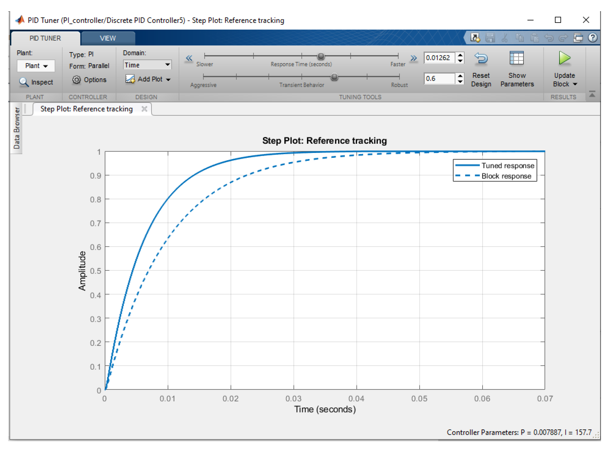
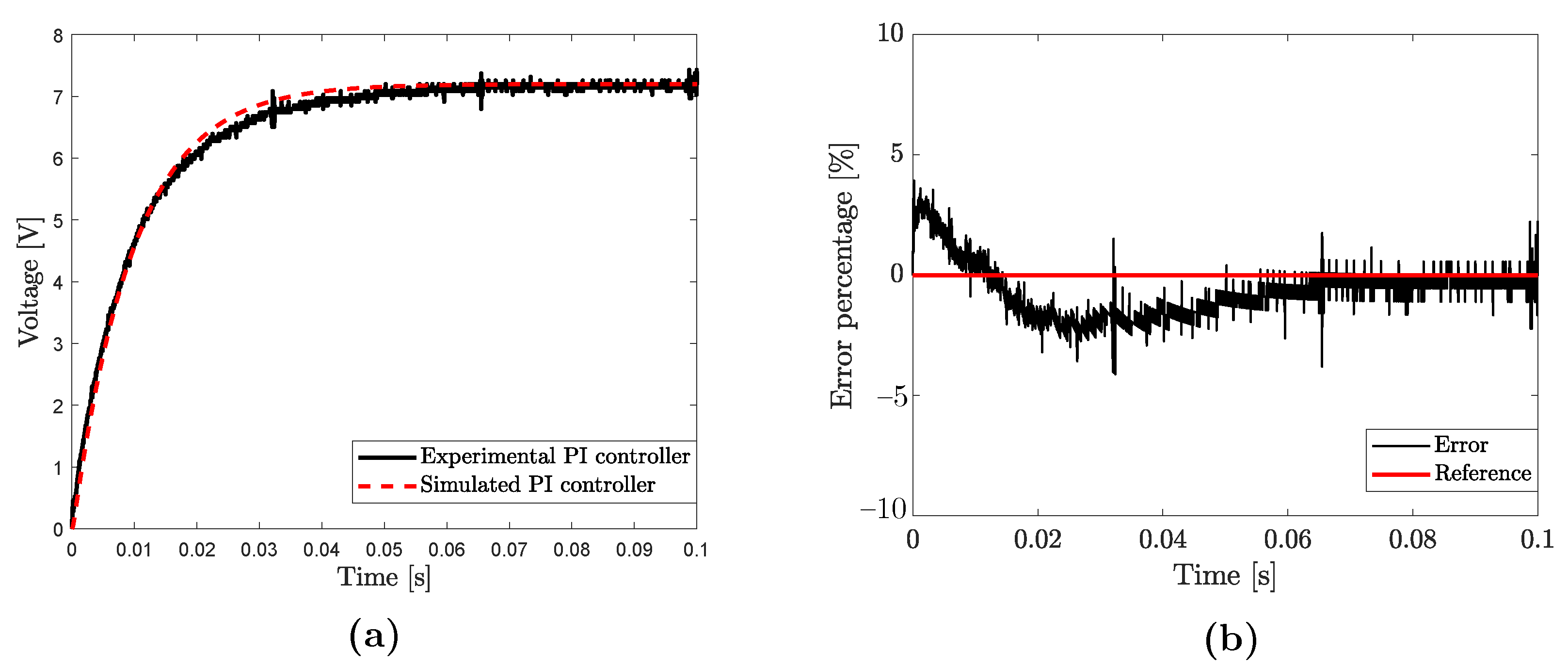
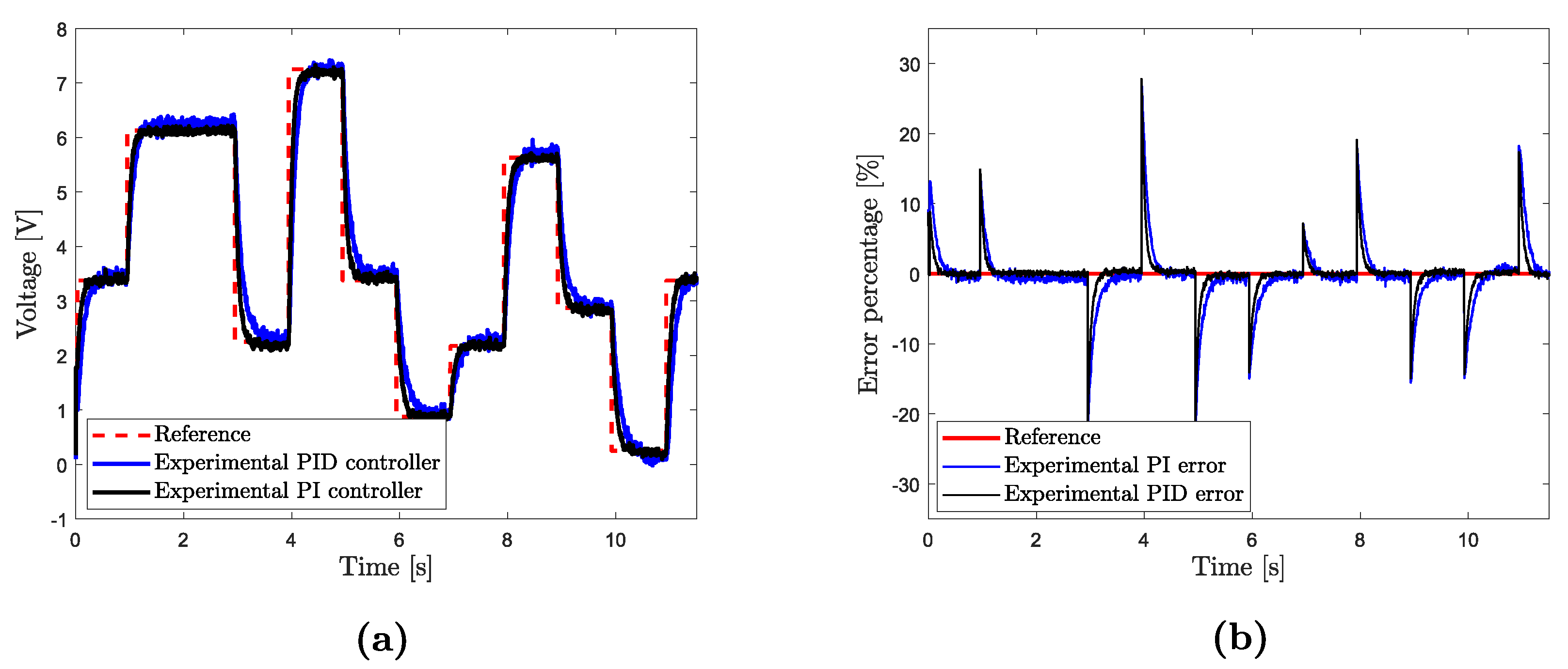
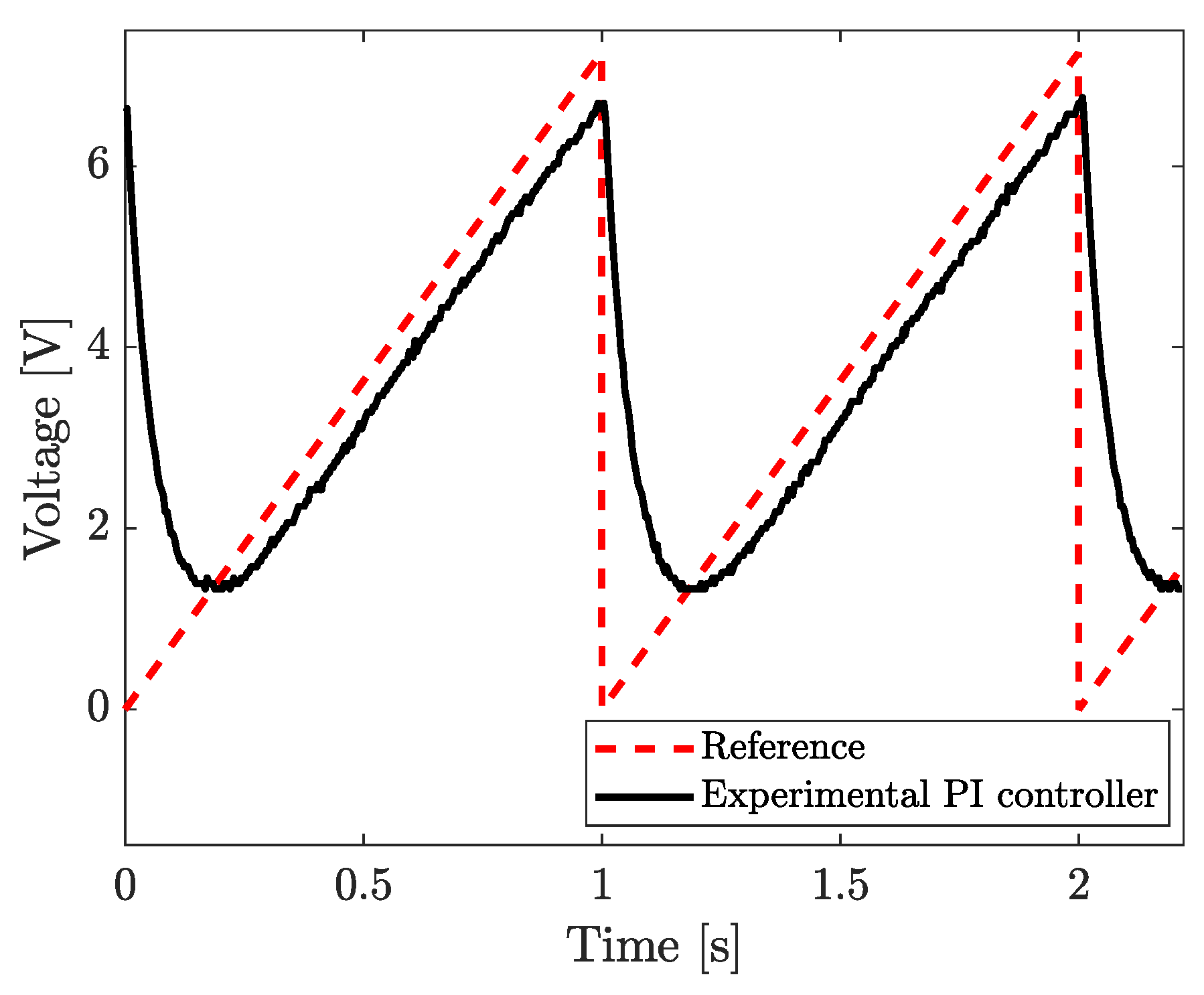
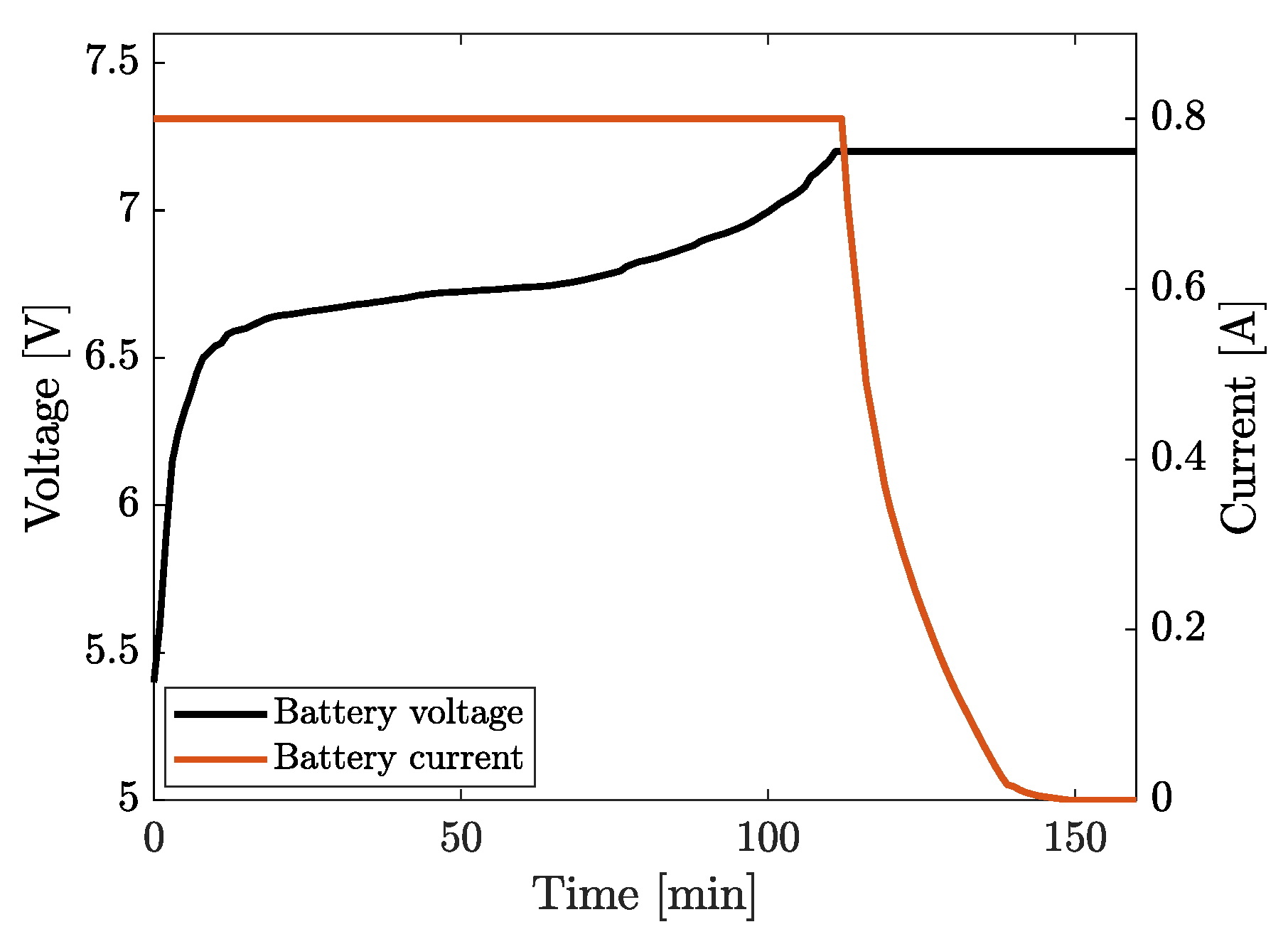
3.3. Voltage Control

For this plant, a classic controller is used to adjust the converter voltage. Being a discrete control, the transfer function of the controller can be expressed in different ways in the integral and derivative part.
The integral term can be expressed in the following ways:
K i T S z 1 Forward Euler
K i T S z z 1 Backward Euler
K i T S 2 z + 1 z 1 Trapezoidal
The forward Euler form is considered and the controller proposed for this application is a PI controller.
The transfer function of the controller would be as follows:
G C ( z ) = K p ( z 1 ) + K i T S z 1
The diagram where the model and the controller are contemplated is shown in Figure 7. The load is the battery in the graph, and the controller regulates the voltage supplied to the battery. However, to tune the controller, a resistor is used to observe the voltage variation across the system and the response time of the controller.
The response of the system is determined by the values that are assigned to K p and K i . Two possible control approaches are considered. The first test is carried out considering a rise time of 20 ms, which is shown in Figure 8. MATLAB’s PID Tuner was used to determine the values for K p and K i . The tuner is shown in Figure 9. The obtained values are:
K p = 0.011945 K i = 238.83
The expected response and the one obtained are quite similar, which is an indicator that the modeling was carried out correctly.
However, by proposing a faster system response, the integral part does not allow the plant to sustain a constant voltage. For this reason, it is considered a slower response, since in this application a response of 20 ms is not critical, because the battery voltage does not change faster than the response of the system.
A second test is performed, but this time considering a rise time of 50 ms. In this case the values of the proportional and integral terms are:
K p = 0.0049 K i = 99.73
The controller behaves as shown in Figure 10. In this case, the voltage becomes adjusted with a lower error range, and the theoretical response becomes quite close to the real one. Although the response of the controller is slower, it does not affect the application in question since the battery voltage also changes slowly.
Therefore, it can be concluded that the controller must consider a rise and settling time of more than 50 ms to avoid having a large margin of error.
Next, it is necessary to test the dynamic response of the system to verify the regulation capability of the controller. The first test is to change the setpoint to a random step signal, and the second one is to change the setpoint to a sawtooth signal.
By changing the setpoint to a random step signal, the following results are obtained:
The controller behaves in the same way as when a step signal is input to it. The difference in this test is that the controller must constantly adjust to different setpoints. The controller manages to adjust to the different variations correctly. For a more accurate comparison, the PI controller is compared to a PID controller. In this case, the PID controller is designed to have the same rising time as the PI controller. A random step signal is used as well to analyze the behavior of the controller. The responses are shown in Figure 11a.
When looking at the PID controller, a little distortion is observed in the output voltage. This is mainly because the derivative part has been incorporated into the controller, introducing noise to the signal. This is why the PI controller is considered to be more suitable for this application.
Now, the setpoint is changed to a sawtooth signal as shown in Figure 12. In this particular case, it is more difficult for the PI controller to adjust to the reference when it changes drastically. A different tuning or a more complex controller might be needed to be able to adjust to these abrupt changes.
Finally a test is done by charging a two-cell LiFePO 4 battery. In this case the constant-voltage constant-current (CV-CC) method is used to charge the battery. The same controller is used to control the PSFB current and a condition is set in the microcontroller to switch between voltage control and current control. Results can be seen in Figure 13.

4. Conclusions

This research presents the modeling and control of a PSFB converter using the ARX model and a classical controller. The modeling and control meet the charging requirements of a LiFePO 4 battery. The modeling gets to describe the plant with a precision of 94%. Therefore, the designed controller resembles the one obtained in experimental results in the two proposed cases. The controller behaves precisely, reaching an accuracy of 96% and controlling the output voltage as expected.
The ARX model was tested by comparing the expected and the actual response with a step input. A comparison was also made in relation to frequency between the real and the modeled response, where both behave the same way. The controller was put to the test by considering different reference points, achieving the expected results when a step signal, a random signal and a sawtooth signal were introduced. This allows the obtained model to be experimentally demonstrated.
The integral part of the controller can govern the response time of the system. However, reducing the rise time prevents the voltage from being regulated correctly. Using the ARX model facilitates the implementation of the controller in any embedded system since the equations used are in discrete time. LiFePO 4 cell charging verifies the correct operation of the controller by properly regulating both voltage and current. The selected charging method allows the same model to be used to regulate both the converter voltage and current. Future work intends to implement a fuzzy controller to observe the impact of this controller on the application.

Author Contributions

Conceptualization, I.A.M.-V. and M.A.M.-P.; methodology, I.A.M.-V.; software, I.A.M.-V.; validation, I.A.M.-V. and M.A.M.-P.; formal analysis, I.A.M.-V., A.A.-D. and M.A.M.-P.; investigation, I.A.M.-V.; resources, I.A.M.-V. and J.R.-R.; data curation, I.A.M.-V.; writing—original draft preparation, I.A.M.-V. and J.R.-R.; writing—review and editing, A.A.-D. and M.A.M.-P.; visualization, I.A.M.-V.; supervision, A.A.-D. and J.R.-R.; project administration, M.A.M.-P.; funding acquisition, M.A.M.-P. All authors have read and agreed to the published version of the manuscript.

Funding

This research was funded by CONACYT.

Acknowledgments

Thanks to the Autonomous University of Queretaro (UAQ) and the Faculty of Engineering for its support to carry out this research.

Conflicts of Interest

The authors declare no conflict of interest.

References

  1. Instituto Nacional de Estadística y Geografía. Registro Administrativo de la Industria Automotriz de Vehículos Ligeros; Instituto Nacional de Estadística y Geografía: Aguascalientes City, Mexico, 2020.
  2. Solaymani, S. CO2 emissions patterns in 7 top carbon emitter economies: The case of transport sector. Energy 2019, 168, 989–1001. [Google Scholar] [CrossRef]
  3. Wang, J.; Sun, X. Understanding and recent development of carbon coating on LiFePO4 cathode materials for lithium-ion batteries. Energy Environ. Sci. 2012, 5, 5163–5185. [Google Scholar] [CrossRef]
  4. Scrosati, B.; Garche, J. Lithium batteries: Status, prospects and future. J. Power Sources 2010, 195, 2419–2430. [Google Scholar] [CrossRef]
  5. Yilmaz, M.; Krein, P.T. Review of Battery Charger Topologies, Charging Power Levels, and Infrastructure for Plug-In Electric and Hybrid Vehicles. IEEE Trans. Power Electron. 2013, 28, 2151–2169. [Google Scholar] [CrossRef]
  6. Khaligh, A.; D’Antonio, M. Global Trends in High-Power On-Board Chargers for Electric Vehicles. IEEE Trans. Veh. Technol. 2019, 68, 3306–3324. [Google Scholar] [CrossRef]
  7. Kumar, D.; Nema, R.K.; Gupta, S. A comparative review on power conversion topologies and energy storage system for electric vehicles. Int. J. Energy Res. 2020, 44, 7863–7885. [Google Scholar] [CrossRef]
  8. Choudhury, T.; Nayak, B.; De, A. A comprehensive review and feasibility study of DC–DC converters for different PV applications: ESS, future residential purpose, EV charging. Energy Syst. 2020, 11, 641–671. [Google Scholar] [CrossRef]
  9. Lee, J.; Kim, J.M.; Yi, J.; Won, C.Y. Battery Management System Algorithm for Energy Storage Systems Considering Battery Efficiency. Electronics 2021, 10, 1859. [Google Scholar] [CrossRef]
  10. Ortega, M.; Jurado, F.; Vera, D. Novel topology for DC-DC full-bridge unidirectional converter for renewable energies. IEEE Latin Am. Trans. 2014, 12, 1381–1388. [Google Scholar] [CrossRef]
  11. Phan, N.T.; Nguyen, A.D.; Liu, Y.C.; Chiu, H.J. An Investigation of Zero-Voltage-Switching Condition in a High-Voltage-Gain Bidirectional DC–DC Converter. Electronics 2021, 10, 1940. [Google Scholar] [CrossRef]
  12. Cho, Y.; Jang, P. Analysis and Design for Output Voltage Regulation in Constant-on-Time-Controlled Fly-Buck Converter. Electronics 2021, 10, 1886. [Google Scholar] [CrossRef]
  13. Oh, C.; Kim, D.; Woo, D.; Sung, W.; Kim, Y.; Lee, B. A High-Efficient Nonisolated Single-Stage On-Board Battery Charger for Electric Vehicles. IEEE Trans. Power Electron. 2013, 28, 5746–5757. [Google Scholar] [CrossRef]
  14. Whitaker, B.; Barkley, A.; Cole, Z.; Passmore, B.; Martin, D.; McNutt, T.R.; Lostetter, A.B.; Lee, J.S.; Shiozaki, K. A High-Density, High-Efficiency, Isolated On-Board Vehicle Battery Charger Utilizing Silicon Carbide Power Devices. IEEE Trans. Power Electron. 2014, 29, 2606–2617. [Google Scholar] [CrossRef]
  15. Bosso, J.E.; Oggier, G.G.; Garcia, G.O. Isolated Buck/Boost Bidirectional DC-Three Phase Topology. IEEE Latin Am. Trans. 2016, 14, 2669–2674. [Google Scholar] [CrossRef]
  16. Akter, P.; Uddin, M.; Mekhilef, S.; Tan, N.M.L.; Akagi, H. Model predictive control of bidirectional isolated DC–DC converter for energy conversion system. Int. J. Electron. 2015, 102, 1407–1427. [Google Scholar] [CrossRef] [Green Version]
  17. Al-Haj Hussein, A.; Batarseh, I. A Review of Charging Algorithms for Nickel and Lithium Battery Chargers. IEEE Trans. Veh. Technol. 2011, 60, 830–838. [Google Scholar] [CrossRef]
  18. Jadli, U.; Mohd-Yasin, F.; Moghadam, H.A.; Pande, P.; Chaturvedi, M.; Dimitrijev, S. A Method for Selection of Power MOSFETs to Minimize Power Dissipation. Electronics 2021, 10, 2150. [Google Scholar] [CrossRef]
  19. Lopez, J.C.; Ortega, M.; Jurado, F. New topology for DC/DC bidirectional converter for hybrid systems in renewable energy. Int. J. Electron. 2015, 102, 418–432. [Google Scholar] [CrossRef]
  20. Chou, H.H.; Chen, H.L.; Fan, Y.H.; Wang, S.F. Adaptive On-Time Control Buck Converter with a Novel Virtual Inductor Current Circuit. Electronics 2021, 10, 2143. [Google Scholar] [CrossRef]
  21. Kim, H.Y.; Kim, T.U.; Choi, H.Y. A Two-Channel High-Performance DC-DC Converter for Mobile AMOLED Display Based on the PWM–SPWM Dual-Mode Switching Method. Electronics 2021, 10, 2059. [Google Scholar] [CrossRef]
  22. Ruan, X. Soft-Switching PWM Full-Bridge Converters; John Wiley and Sons Singapore Pte. Ltd.: Singapore, 2014. [Google Scholar]
  23. Di Capua, G.; Shirsavar, S.A.; Hallworth, M.A.; Femia, N. An Enhanced Model for Small-Signal Analysis of the Phase-Shifted Full-Bridge Converter. IEEE Trans. Power Electron. 2015, 30, 1567–1576. [Google Scholar] [CrossRef]
  24. Tomesc, L.; Betea, B.; Dobra, P. Determining the Frequency Response of a DC-DC Converter thru System Identification. IFAC Proc. Vol. 2013, 46, 149–152. [Google Scholar] [CrossRef]
  25. Amran, M.; Bakar, A.; Jalil, M.; Wahyu, M.; Gani, A. Simulation and modeling of two-level DC/DC boost converter using ARX, ARMAX, and OE model structures. Indones. J. Electr. Eng. Comput. Sci. 2020, 18, 1172–1179. [Google Scholar] [CrossRef]
  26. O’Loughlin, M. Phase-Shifted, Full-Bridge Application Report; Technical Report SLUA560C; Texas Instruments: Dallas, TX, USA, 2011. [Google Scholar]
Figure 1. PSFB DC-DC Converter.
Electronics 10 02568 g001
Figure 2. Switching control signals.
Electronics 10 02568 g002
Figure 3. Test bench used for experimentation.
Electronics 10 02568 g003
Figure 4. ARX model obtained on second, third, and fourth order.
Electronics 10 02568 g004
Figure 5. Plant response to step input. (a) Comparison between real and modeled response. (b) Error obtained by comparing the real response and the modeled response.
Electronics 10 02568 g005
Figure 6. Comparison between protype and obtained model regarding frequency response.
Electronics 10 02568 g006
Figure 7. System diagram, considering the model obtained and the voltage controller.
Electronics 10 02568 g007
Figure 8. Case 1 with T s = 0.02 . (a) Controller response. (b) Error obtained by comparing the simulated controller and the experimental controller.
Electronics 10 02568 g008
Figure 9. Controller tuning via PID Tuner from MATLAB.
Electronics 10 02568 g009
Figure 10. Case 2 with T s = 0.05 . (a) Controller response. (b) Error obtained by comparing the simulated controller and the experimental controller.
Electronics 10 02568 g010
Figure 11. Response to random step signal. (a) Controller response, PI and PID case. (b) Error obtained by comparing the simulated controllers and the experimental controllers.
Electronics 10 02568 g011
Figure 12. PI controller response to sawtooth signal.
Electronics 10 02568 g012
Figure 13. LiFePO 4 battery charged via CV-CC.
Electronics 10 02568 g013
Table 1. Comparison of isolated converters [22].
ConverterVoltage Stressof SwitchesCurrent Stressof SwitchesSwitchesFrequency
Simple forward2 V i n I o / n 1 f s
Double forward V i n I o / n 2 f s
Push–pull2 V i n I o / ( 2 n ) 22 f s
Half bridge V i n I o / n 22 f s
PSFB V i n I o / ( 2 n ) 42 f s
Where I o is the output current, n is the transformer winding turns ratio, f s is the switching frequency.
Table 2. Previous work on identifying DC-DC converters.
Identification MethodSystem to Be ModeledVerification MethodReference
Proposed dynamic modelPSFB ConverterExperimental[23]
ARX modelBuck converterResidual autocorrelation[24]
ARX, ARMAX, OE modelTwo level boost converterSimulation[25]
Table 3. Components of test bench.
ComponentType
MicrocontrollerB-G474E-DPOW1
Output inductor100 µH
Output capacitor3000 µF
Ferrite coreETD49
MOSFETSTP36N55M5
DiodeRHRP3060
Publisher’s Note: MDPI stays neutral with regard to jurisdictional claims in published maps and institutional affiliations.

