Novel Method of Coupling Coefficient Estimation Based on the Bifurcation Phenomena in Inductive Power Transfer

Abstract

Inductive power transfer (IPT) applications, such as stationary charging of electric vehicles (EVs), at least moderate coupling between the coils to achieve high efficiency, but the coefficient $k$ typically varies between of 0.1 to 0.4, depending on the displacement of the coils according to SAE J2954. Thus, accurate and reliable methods for estimation of $k$ are required for positioning of the EV to achieve optimal alignment with the charging pad. Additionally, in IPT, numerous control strategies are available for regulating output power and optimizing system efficiency that require an accurate estimate of the mutual inductance or $k$. However, existing estimation methods tend to require detailed a-priori information of a large number of circuit parameters, or they need measurement of currents or voltages in both primary and secondary sides. This paper presents a preliminary evaluation of a novel, primary-side method to estimate $k$, which is based solely on the frequency response of the input phase while operating the system in bifurcation. The method does not require any additional measurements of the system parameters. The theoretical background of the method is presented together with the description of the measurement procedure. The method is experimentally verified and compared with two currently used estimation methods. According to the presented experimental evaluation, the proposed method estimates $k$ with an error of 3.62% with respect to the reference over the evaluated range of 0.08 to 0.36. In addition, we demonstrate that the presented method is resilient to detuning.

1. Introduction

Inductive power transfer (IPT) is a developing technology for simplifying and streamlining the electric vehicle (EV) charging experience [1,2,3]. Based on the movement of the vehicle, this application can be divided in dynamic, semi-dynamic or stationary charging [4,5]. In dynamic charging, an EV is charged while it travels over an electrified road [6]. Multiple scenarios of the electrification track are possible: it can be formed by a single elongated primary coil (similar to materials handling systems), or by segmented track, where each segment powered or switched individually, or by a sequence of pads similar to those used for EV charging [6,7,8].

Semi-dynamic charging is derived from the dynamic charging, but instead of powering vehicles in-move, they are powered at the intersections, traffic lights or bus stops (electrified public transport vehicles), where the vehicles are temporary stationary [4].

Stationary IPT chargers replace conductive chargers and can be fully integrated in the parking space, so that no part of the charger is visible [9]. Several standards were developed for stationary EV charging, e.g., SAE J2954 [10] or IEC 61980 [11]. The modern IPT systems for EV charging achieve similar levels of efficiency (>90%) and transferred power (tens and hundreds of kW) as the conductive chargers [2,12,13,14].

Unfortunately, the power transfer capability and efficiency of IPT systems are dependent on the coil alignment [15]. Thus, to ensure sufficient efficiency, the coils need to be correctly positioned [10], which requires feedback of their position or, preferably, the coupling coefficient $k$. Additionally, several control algorithms have been proposed, such as [16,17], which aim to provide power regulation and optimize efficiency under coil displacement. However, they require the value of the coupling coefficient $k$ or mutual inductance $M$ for operation.

There are several methods for estimating the coupling coefficient $k$ [18,19,20,21], but they usually require knowledge of a large number circuit parameters [18,20,21] or require voltage or current information from both the transmitter and receiver [19]. If these parameters are measured inaccurately or they change (e.g., due to the displacement or temperature), the estimate quality will decrease. Also, some of the methods are based on complicated procedures requiring increased computational power [19,20].

In this paper, we present a preliminary evaluation of a novel primary-sided method for estimating the coupling coefficient, which is based solely on the frequency response of the input phase while the IPT system is intentionally operated in bifurcation. The proposed method also requires only a minimal number of calculations.

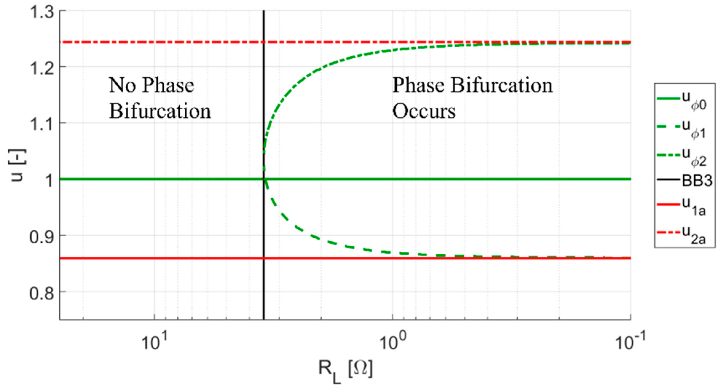
Bifurcation is a phenomenon during which the single frequency at which the input current is in phase with voltage, splits into three such frequencies. These frequencies are called the zero-phase angle (ZPA) frequencies. The original ZPA frequency is the resonance frequency $f_0$, and the additional ZPA frequencies are denoted $f_{\phi 1}$ and $f_{\phi 2}$ in this work. The ZPA frequency $f_{\phi 1}$ is lower than $f_0$, and $f_{\phi 2}$ is higher than $f_0$. The onset of bifurcation can be initiated for example by appropriately adjusting the load or coupling coefficient $k$. As bifurcation increases, the ZPA frequencies $f_{\phi 1}$ and $f_{\phi 2}$ approach their respective asymptotes $f_{1\mathrm{a}}$ and $f_{2\mathrm{a}}$, which are functions solely of the coupling coefficient $k$ and $f_0$.

The proposed method is developed and applied for the series–series (SS) compensated IPT system. The most practical way to achieve deep bifurcation for the SS compensation is to short-circuit the output. Under such a condition, the frequency response of the input phase ${\phi }_{in}$ is measured to find the ZPA frequencies $f_{\phi 1}\approx f_{1\mathrm{a}}$ and $f_{\phi 2}\approx f_{2\mathrm{a}}$, which are then used to calculate the coupling coefficient $k$.

Since the method requires shorting the load, the method would not be used while power is being transferred to the EV. Instead, this method is applicable for initial estimation of $k$ during start-up (i.e., before the charging begins) or intermittent estimation of $k$ (i.e., in between periods of charging). In practice, the load could be short circuited using an active rectifier (in which both of the bottom transistors are turned on), through the DC/DC converter between the rectifier and EV battery, or a dedicated switch at the DC side after the rectifier.

In comparison with the current estimation methods, the proposed method requires (coarse) measurement of the frequency response of the input phase. However, its main advantage is that it does not require a-priori information about the system (except for an approximate frequency range for the frequency response measurement). It also requires only the primary side information (i.e., no wireless feedback between the secondary and primary is needed). The preliminary measurement results presented in this paper also show that the method is resilient to the detuning due to change of inductances in displacement. The method’s estimate of $k$ only differed from the reference value by an average absolute error of 3.62% over the range $k=$ 0.08 to $k=$ 0.36.

The second chapter of the paper describes the initial AC equivalent circuit model, of which the method is based. The third chapter follows by deriving of the asymptotes of the ZPA frequencies $f_{\phi 1}$ and $f_{\phi 2}$. The fourth chapter outlines the presented method itself, which is then experimentally verified in the fifth chapter and compared to the selected currently used methods for coupling coefficient estimation. The practical aspects of the selected methods are further discussed in the sixth chapter.

2. AC Equivalent Circuit

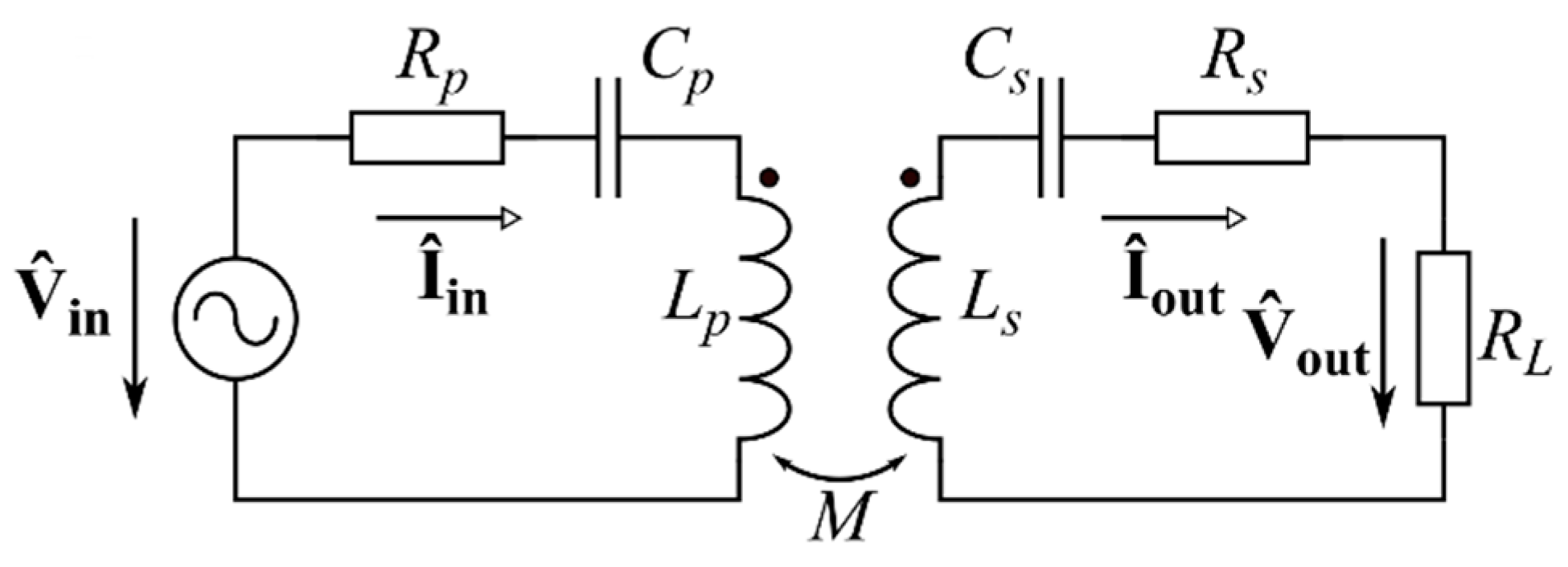
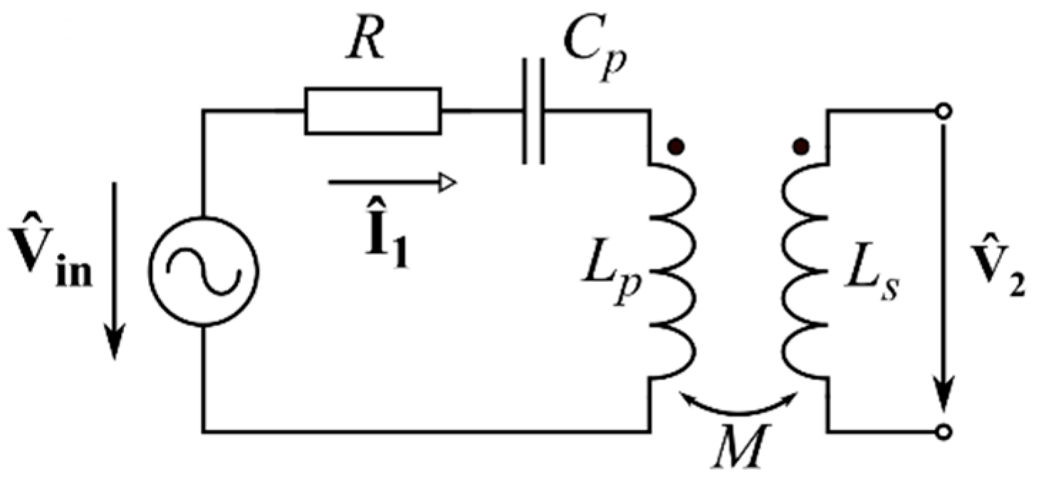
The proposed $k$-parameter estimation method is based on the AC equivalent circuit model of the IPT system depicted in Figure 1. The arrangement represents a single transmitter and receiver with the series–series compensation topology. The primary and secondary coil inductances $L_p$ and $L_s$, respectively, are compensated by capacitances $C_p$ and $C_s$ to form series resonant circuits with resonant frequencies $f_p$ and $f_s$. The frequencies $f_p$ and $f_s$ are set to the same value of $f_0$, which is the common resonant frequency $f_0$. The capacitances $C_p$ and $C_s$ are then calculated as:

$$C_p=\frac{1}{{\omega }_{0p}^2{L}_p}$$

(1)

$$C_s=\frac{1}{{\omega }_{0s}^2{L}_s}$$

(2)

where ${\omega }_{0p}={\omega }_{0s}={\omega }_0=2\pi f_0$ for the primary tuned to the secondary.

Figure 1. Equivalent AC circuit schematics for the series–series compensated IPT system.

The coils are coupled by the mutual inductance $M$. The circuit is loaded by a purely resistive load, which is represented in Figure 1 by the equivalent load resistance $R_L$. The equivalent series resistances (ESRs) representing losses of each side are summarized in $R_p$ and $R_s$. The circuit is powered from a source, which is considered sinusoidal (first harmonic approximation). Therefore, all the voltages and currents are represented by phasors, which are marked as $\widehat{X}$. The symbol $X$ without this marking refers to phasor amplitude. The input voltage ${\widehat{V}}_{in}$ is described by its amplitude $V_{in}$, its frequency $f$ (the operating frequency of the circuit) and its phase ${\phi }_{in}$ with respect to the input current ${\widehat{I}}_{in}$, which is taken as the reference. $V_{in}$ is considered constant. The IPT system output is characterized by the output voltage ${\widehat{V}}_{out}$ and current ${\widehat{I}}_{out}$.

The input impedance of the circuit in Figure 1 is described by:

$$\widehat{Z}=Re\left\{\widehat{Z}\right\}+j·Im\left\{\widehat{Z}\right\}=\frac{{\omega }^4{C}_s^2{M}^2{R}_{sL}}{{\left({\omega }^2{C}_s{L}_s-1\right)}^2+{\omega }^2{C}_s^2{R}_{sL}^2}+j\left(\omega L_1-\frac{1}{\omega C_p}-\frac{{\omega }^3{C}_s{M}^2\left({\omega }^2{C}_s{L}_s-1\right)}{{\left({\omega }^2{C}_s{L}_s-1\right)}^2+{\omega }^2{C}_s^2{R}_{sL}^2}\right)$$

(3)

3. Theoretical Background of the Estimation Method

As discussed in the introduction, the phase bifurcation is the splitting of a single ZPA frequency into three. Specifically, the ZPA frequencies are described by condition:

$$Im\left\{\widehat{Z}\right\}=0$$

(4)

The formulas describing the phase bifurcation frequencies can be obtained from (4). To simplify the calculation, the normalization process presented by Wang et al. in [22] can be advantageously used. In the normalization, the ESRs $R_p$ and $R_s$ are neglected. The IPT model is normalized as follows. First, the normalized operating frequency $u$ is defined as the operating frequency $f$ divided by $f_0$:

$$u=\frac{f}{f_0}$$

(5)

Second, the imaginary part of the input impedance $Im\left\{\widehat{Z}\right\}$ is divided by the real part of the reflected impedance at resonance $Re\left\{{\widehat{Z}}_{r0}\right\}$ to obtain normalized $Im\left\{{\widehat{Z}}_n\right\}$:

$$Im\left\{{\widehat{Z}}_n\right\}=\frac{Im\left\{\widehat{Z}\right\}}{Re\left\{{\widehat{Z}}_{r0}\right\}}$$

(6)

$$Re\left\{{\widehat{Z}}_{r0}\right\}=\frac{{\omega }_0^2{M}^2}{R_L}$$

(7)

A series of substitutions is then applied after which $Im\left\{\widehat{Z}\right\}$ is expressed solely in terms of $u$ and the loaded quality factors $Q_{Lp}$ and $Q_{Ls}$, which are defined as:

$$Q_{Lp}=\frac{R_L{L}_p}{{\omega }_0{M}^2}, Q_{Ls}=\frac{{\omega }_0{L}_s}{R_L}$$

(8)

In the last step, Equation (4) is transformed into the phase bifurcation equation by substituting $Im\left\{{\widehat{Z}}_n\right\}$ for $Im\left\{\widehat{Z}\right\}$:

$$\frac{\left(u^2-1\right)\left(\left(Q_{Lp}{Q}_{Ls}^2-Q_{Ls}\right)u^4+\left(Q_{Lp}-2Q_{Lp}{Q}_{Ls}^2\right)u^2+Q_{Lp}{Q}_{Ls}^2\right)}{u{\left(u^2-1\right)}^2{Q}_{Ls}^2+u^3}=0$$

(9)

The detailed derivation of the phase bifurcation equation is described in [22].

When solved for $u$, Equation (9) has six roots, three positive ones and three negative ones. The negative roots are neglected as $u$ cannot be negative. The first root $u_{\phi 0}=1$ describes the resonance frequency $f_0$, and second and third roots describe the ZPA frequencies $u_{\phi 1}$ and $u_{\phi 2}$, respectively:

$$u_{\phi 1}=\sqrt{\frac{2Q_{Lp}{Q}_{Ls}^2-\sqrt{Q_{Lp}\left(4Q_{Ls}^3-4Q_{Lp}{Q}_{Ls}^2+Q_{Lp}\right)}-Q_{Lp}}{2Q_{Ls}\left(Q_{Lp}{Q}_{Ls}-1\right)}}$$

(10)

$$u_{\phi 2}=\sqrt{\frac{2Q_{Lp}{Q}_{Ls}^2+\sqrt{Q_{Lp}\left(4Q_{Ls}^3-4Q_{Lp}{Q}_{Ls}^2+Q_{Lp}\right)}-Q_{Lp}}{2Q_{Ls}\left(Q_{Lp}{Q}_{Ls}-1\right)}}$$

(11)

and when the roots $u_{\phi 1}$ and $u_{\phi 2}$ become real, the phase bifurcation occurs.

Analyzing Equations (10) and (11) for the ZPA frequencies $u_{\phi 1}$ and $u_{\phi 2}$ shows that these frequencies are asymptotic and that the asymptotes depend solely on the coupling coefficient $k$. The asymptotic behavior can be demonstrated by decreasing the equivalent load resistance $R_L$ towards zero. Figure 2 for IPT system described in Section 5.1. shows the course of the ZPA frequencies $u_{\phi 0}$, $u_{\phi 1}$ and $u_{\phi 2}$ with decreasing $R_L$ while the remaining equivalent circuit parameters remain constant. As it can be seen, the ZPA frequencies $u_{\phi 1}$ and $u_{\phi 2}$ begin close to the resonance frequency $u_0$. As $R_L$ decreases further, $u_{\phi 1}$ and $u_{\phi 2}$ recede until they stabilize at the asymptotes. The deep bifurcation, i.e., very low $R_L$, is required for the roots of the bifurcation equation approach the asymptotes closely. The easiest way to achieve this is to short-circuit the output of the IPT system.

Figure 2. The course of bifurcation with decreasing load resistance $R_L$. The normalized frequency $u_0$ corresponds to the resonance frequency $f_0$, while $u_{\phi 1}$ and $u_{\phi 2}$ with higher ZPA frequencies $f_{\phi 1}$ and $f_{\phi 2}$, respectively. Their asymptotes are $u_{1a}$ and $u_{2a}$, respectively.

To obtain the equation for the coupling coefficient $k$ calculation, it is necessary to obtain the formulas for the asymptotes. In the first step, the loaded quality factors $Q_{Lp}$ and $Q_{Ls}$ given by (8) are substituted in the roots $u_{\phi 1}$ and $u_{\phi 2}$ of the bifurcation equation, which are given by (10) and (11), respectively. Then their asymptotic values are calculated in the limit as $R_L$ goes to zero. In the next step the normalized frequency $u$ given by (5) is substituted together with the coupling coefficient $k$:

$$k=\frac{M}{\sqrt{L_1{L}_2}}$$

(12)

The final results are the equations for the asymptotes $f_{1a}$ and $f_{2a}$:

$$f_{1a}=\frac{f_0}{\sqrt{1+k}}$$

(13)

$$f_{2a}=\frac{f_0}{\sqrt{1-k}}$$

(14)

This result is interesting, because the asymptotes of the frequencies describing the frequency splitting of the output power $P_{out}$ maxima can be approximated by a similar set of formulas [23,24]. Our examination of the frequencies of the input current amplitude $I_{in}$ maxima showed that they also have the same asymptotes.

The coupling coefficient $k$ can be calculated from the asymptotes $f_{1a}$ and $f_{2a}$ given by (13) and (14), respectively, as:

$$k=\frac{f_{2a}^2-f_{1a}^2}{f_{2a}^2+f_{1a}^2}$$

(15)

Note that the issue of coupling coefficient extraction is also important in distributed-element filter design; and, as discussed in [25], an equation identical to (16) is used to characterize coupled RF/microwave resonators based on the splitting of the scattering parameter $S_{21}$.

4. Proposed Estimation Method (Bifurcation Asymptotes Method)

Equation (15) can be advantageously used for estimation of the coupling coefficient $k$. Thus, we propose the following procedure based on the bifurcation asymptotes, which estimates $k$ using the frequency response of the input phase ${\phi }_{in}$.

The bifurcation asymptotes method has the following steps:

(1)

Short-circuit the output of the IPT system.

(2)

Find the approximate values of the frequencies $f_{1a}$ and $f_{2a}$ by searching for either zero crossings of ${\phi }_{in}$ or input current amplitude $I_{in}$ maxima with a large step of $f$.

(3)

Measure ${\phi }_{in}$ with increased precision (smaller step of $f$) near the approximated values of $f_{1a}$ and $f_{2a}$.

(4)

For each value of $f_{1a}$ and $f_{2a}$ select the frequency of ${\phi }_{in}<0$ and ${\phi }_{in}>0$ nearest to ${\phi }_{in}=0$. Use a linear approximation to calculate the zero-crossing frequency of ${\phi }_{in}$ (${\phi }_{in}=0$) from the selected frequencies and phases. The obtained frequencies are approximately equal to $f_{1a}$ and $f_{2a}$.

(5)

Apply (15) to calculate the coupling coefficient $k$ from the approximated values of $f_{1a}$ and $f_{2a}$.

The individual steps are examined in further detail in the following discussion. In order to use (15), it is necessary to achieve such values of $Q_{Lp}$ and $Q_{Ls}$ that $f_{\phi 1}$ and $f_{\phi 2}$ would approach $f_{1a}$ and $f_{2a}$, respectively. While there are multiple ways to achieve such a change of $Q_{Lp}$ and $Q_{Ls}$, e.g., by decreasing $f_0$, minimizing of $R_L$ by short-circuiting the output is the most practical.

Because the method is based on measuring the frequency response, a knowledge of a frequency range to examine is necessary. However, this range depends on $k$ based on (13) and (14), which is unknown. We find that it is most convenient is to start at $f_0$, and then extend the search for $f_{1a}$ and $f_{2a}$ both above and below $f_0$. Therefore, an approximate value of $f_0$ is the only information about the IPT system required for the method. An IPT system with $f_0$ of 100 kHz was used for the method verification.

Measurement of the full frequency response with a small step of frequency is time consuming. This could render the method unusable for more dynamic applications. However, because we are only looking for two frequency values (i.e., $f_{1a}$ and $f_{2a}$), it is also unnecessary. To reduce the number of steps, two measures were taken.

At first, a rough approximation of frequencies $f_{1a}$ and $f_{2a}$ is generated by employing a large measurement step—in testing of the method a step of 1 kHz was used. In this search, the positions of $f_{1a}$ and $f_{2a}$ in the frequency range can be evaluated based on multiple criteria. For example, if the evaluation is based on the input phase ${\phi }_{in}$, the positions of $f_{1a}$ and $f_{2a}$ can be localized based on the change of sign of ${\phi }_{in}$. Frequencies $f_{1a}$ and $f_{2a}$ can be also approximated by searching for the frequencies corresponding to maxima of the input current amplitude $I_{in}$, as these have the same asymptotes as the ZPA frequencies $f_{\phi 1}$ and $f_{\phi 2}$. Alternatively, if the primary side DC link current is measured, the frequencies of its maxima can be used as well, as they match $I_{in}$ maxima. In the verification of the presented method, the frequencies of $I_{in}$ maxima were used to generate a first approximation of $f_{1a}$ and $f_{2a}$.

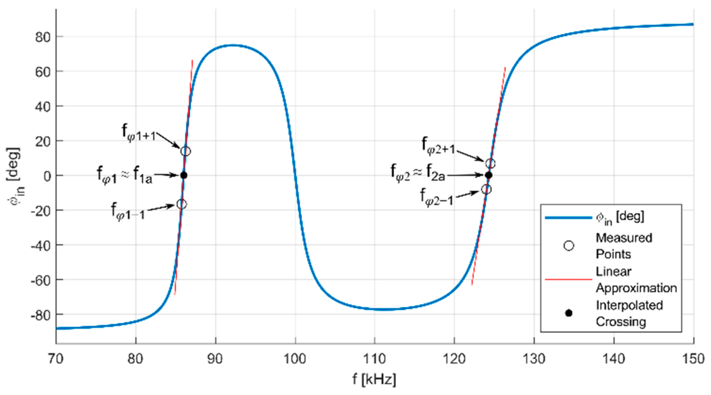
The second measure is to use the linear approximation to find $f_{1a}$ and $f_{2a}$ with increased precision. Figure 3 shows an example of the frequency response of the input phase ${\phi }_{in}$ for deep bifurcation (i.e., $f_{\phi 1}\approx f_{1a}$ and $f_{\phi 2}\approx f_{1a}$) with marked $f_0$, $f_{1a}$ and $f_{2a}$. As the figure shows, the shape of the frequency response ${\phi }_{in}$ is close to linear near the ZPA frequencies $f_{\phi 1}$ and $f_{\phi 2}$.

Figure 3. Frequency response of the input phase ${\phi }_{in}$ for the IPT system in deep bifurcation, with marked measured points, linear approximation and interpolated zero crossings. Based on the circuit parameters from Table 1.

Thus, the values of ${\phi }_{in}$ are measured near the approximated values of $f_{1a}$ and $f_{2a}$ obtained in the first step with a smaller frequency step. In the verification of the method, we measured the ±1 kHz surroundings of the approximated frequencies $f_{1a}$ and $f_{2a}$ with a step of 0.5 kHz. From the resulting data series, the frequencies and phases of the points nearest the zero crossing of ${\phi }_{in}$ were selected for each asymptote: the point $f_{ia-1}$, ${\phi }_{ia-1}$ with phase below zero and the point $f_{ia+1}$, ${\phi }_{ia+1}$ with phase above zero. Both points are marked by hollow circles in Figure 3. From these two points, the values of asymptote frequencies are approximated by:

$$f_{ia}=f_{ia+1}-\frac{f_{ia-1}-f_{ia+1}}{{\phi }_{ia-1}-{\phi }_{ia+1}}{\phi }_{ia+1}$$

(16)

The obtained values of $f_{1a}$ and $f_{2a}$ (full circles in Figure 3) are then used to calculate the coupling coefficient according to (15).

The number of measured frequency points depends on $k$. For example, if $k=0.3$ is measured and $f_0=100$ kHz, then $f_{1a}=87.70$ kHz and $f_{2a}=119.52$ kHz according to (13) and (14), respectively. The first approximation of $f_{1a}$ and $f_{2a}$ with a step of 1 kHz then requires measurement of 34 points and the second refining for the linear approximation requires 10 steps if the ±1 kHz surroundings of frequencies $f_{1a}$ and $f_{2a}$ are measured with a step of 0.5 kHz. In total, 44 points are measured. However, if the method is used to estimate $k$ increasing from a small value (e.g., parking of an EV over a charging station), the number of points can be further reduced by using $f_{1a}$ and $f_{2a}$ estimated from the previous step in the first approximation instead of $f_0$.

Because the asymptotes $f_{1a}$ (13) and $f_{2a}$ (14) are the same for phase bifurcation, frequency splitting of the output power $P_{out}$ maxima and splitting of input current amplitude $I_{in}$ maxima [23,24], alternative approaches to finding the zero crossings of ${\phi }_{in}$ can be used for asymptote approximation, e.g., finding the frequencies of the maxima of $I_{in}$ or $I_{out}$. However, the linear approximation cannot be used to estimate the positions of the maxima; thus, the step of the frequency response would need to be much smaller, resulting in increased measurement time.

5. Experimental Verification

The estimates of $k$ provided by the bifurcation asymptotes method are evaluated with respect to a reference value measured with a calibrated LRC bridge and compared with the results of other active (based on the measurement of currents and voltages) estimation methods. A direct method based on Faraday’s law (i.e., measuring the induced electromotive force (EMF)) and the method introduced by Jiwariyavej et al. in [18] are used for comparison.

In the first part of the chapter, the measurement setup is described together with the measured sequence of coupling coefficients, which is used for evaluation of all three estimation methods. Then, the procedures of the Faraday’s law method and Jiwariyavej’s method are outlined, and the estimation results are compared with the reference for all three selected methods. In the last part of the chapter, the match to the reference of all three methods is evaluated.

5.1. Measurement Setup

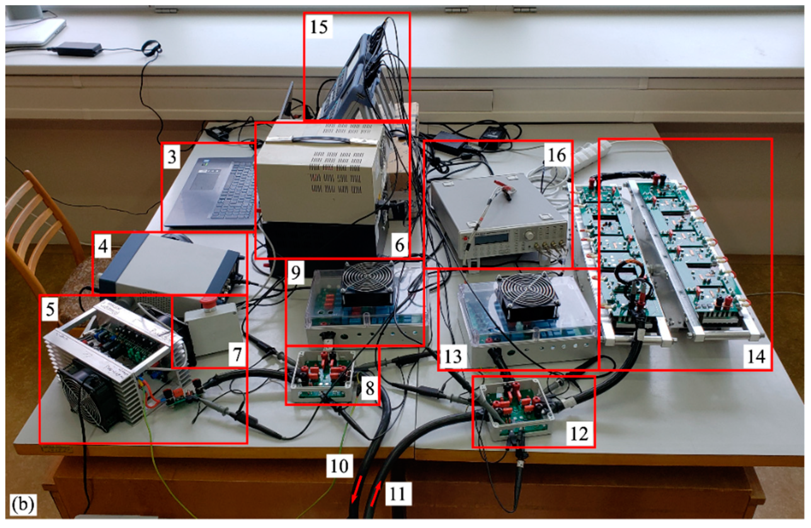
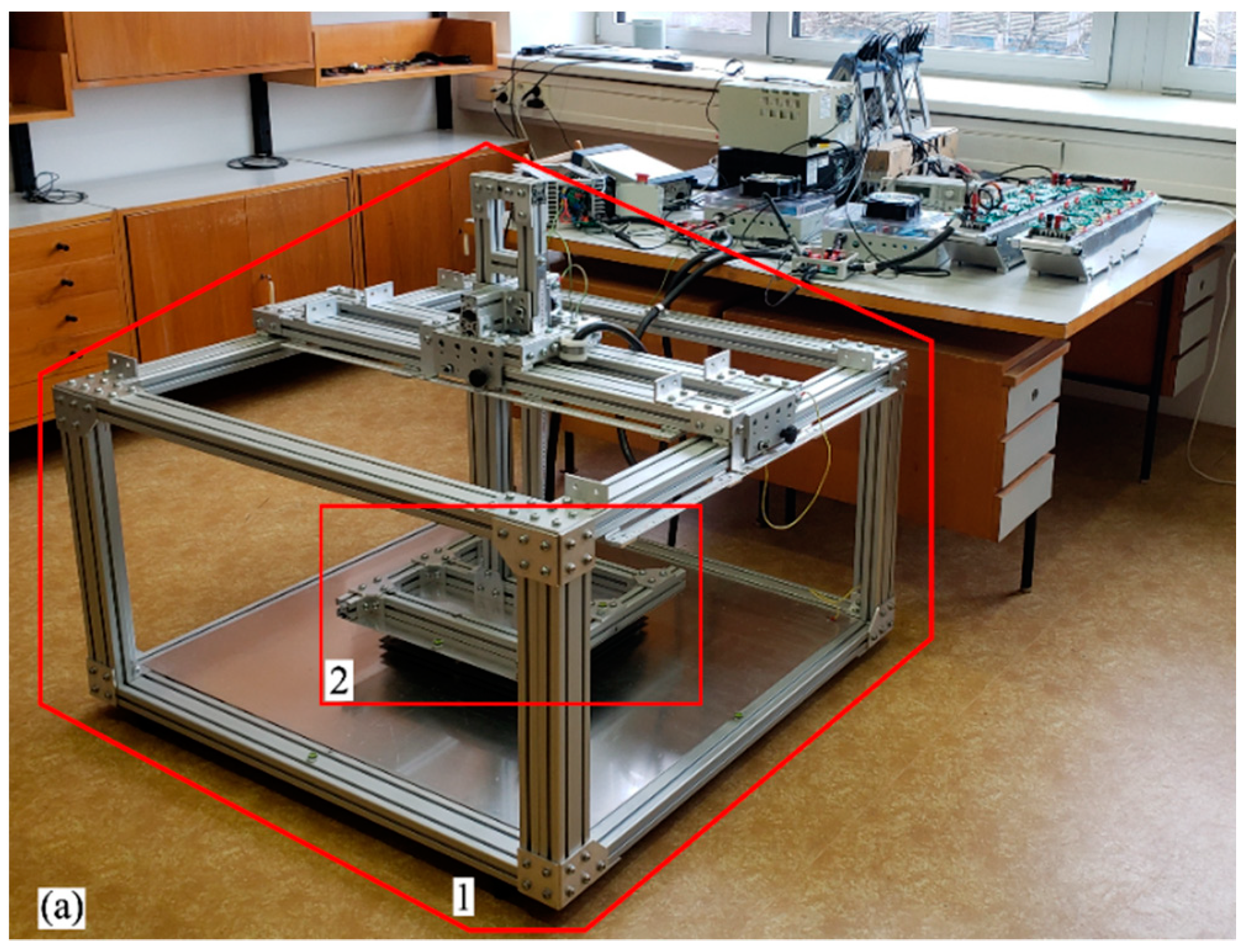
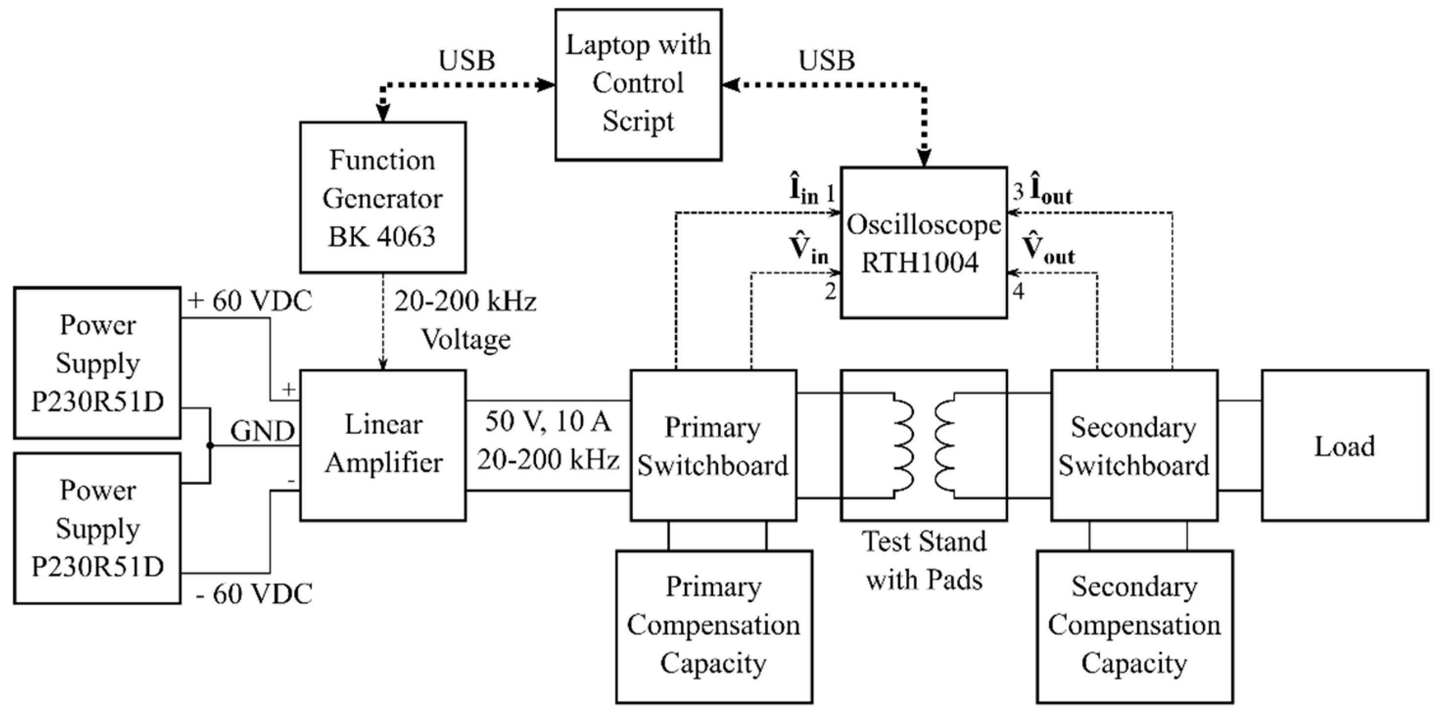
The measured setup used for verification is depicted in Figure 4 (photographs) and in Figure 5 (schematics). The setup was designed to closely resemble the AC equivalent circuit in Figure 1.

Figure 4. Measurement setup. (a) Test stand for coil positioning. 1—Test stand. 2—Pads in the aligned position. (b) Setup without the test stand. 3—Laptop. 4—Function generator. 5—Linear amplifier. 6—Laboratory power sources. 7—Total stop. 8—Primary switchboard. 9—Capacitive decade used as the primary compensation. 10—Cable connecting the primary pad. 11—Cable connecting the secondary pad. 12—Secondary switchboard. 13—Capacitive decade used as the secondary compensation. 14—Resistive decade used as the load. 15—Oscilloscopes. 16—LRC bridge.

Figure 5. Measurement setup block diagram.

The circuit is powered by a linear amplifier driven by the function generator BK Precision 4063 which generates a sinusoidal voltage. The linear amplifier is supplied by power sources Diametral P230R51D. Both the primary and the secondary use DD pads [15,26]. Each coil inductance is compensated by a capacitive decade to provide control over $f_{0p}$ and $f_{0s}$. Nominal resonance frequency was selected as 100 kHz.

The output is loaded by a custom-built resistive decade, designed for high frequency operation. However, for lower values of $R_L$ it has a slight inductive character, but this is considered in $L_s$ and the calculation of $C_s$, which compensates it. The currents are calculated from the measured voltages at current shunts. One of two available oscilloscopes Rohde & Schwarz RTH1004 measures the voltages with RT-ZI10 probes and the shunt voltages corresponding with currents with P2220 probes set to 1:1 attenuation. The voltages are measured at designated points at the switchboards, which connect together all components of each side. The function generator and oscilloscope are controlled by an acquisition MATLAB script running on the laptop. The setup was designed with a focus on the IPT transformer operation and the bifurcation phenomena; thus, the linear amplifier and the resistor decade are used in place of an inverter and output rectifier, respectively. The component parameter values were measured with the LRC bridge Hameg HM8118 with Kelvin probe. The system parameters for the aligned coils (position x = 0 mm) are listed Table 1, except $R_L$, which is specific for each method.

Table 1. System parameters in the position x = 0 mm.

Parameter	Symbol	Value
Input voltage	$V_{in}$	5 V
Primary coil inductance	$L_p$	28.8 µH
Primary compensation capacitance	$C_p$	87.4 nF
Primary ESR	$R_p$	0.23 Ω
Secondary coil inductance	$L_s$	16.7 µH
Secondary compensation capacitance	$C_s$	151.2 nF
Secondary ESR	$R_s$	0.15 Ω
Resonance frequency	$f_0$	100 kHz

5.2. Measured Sequence Used for Method Evaluation

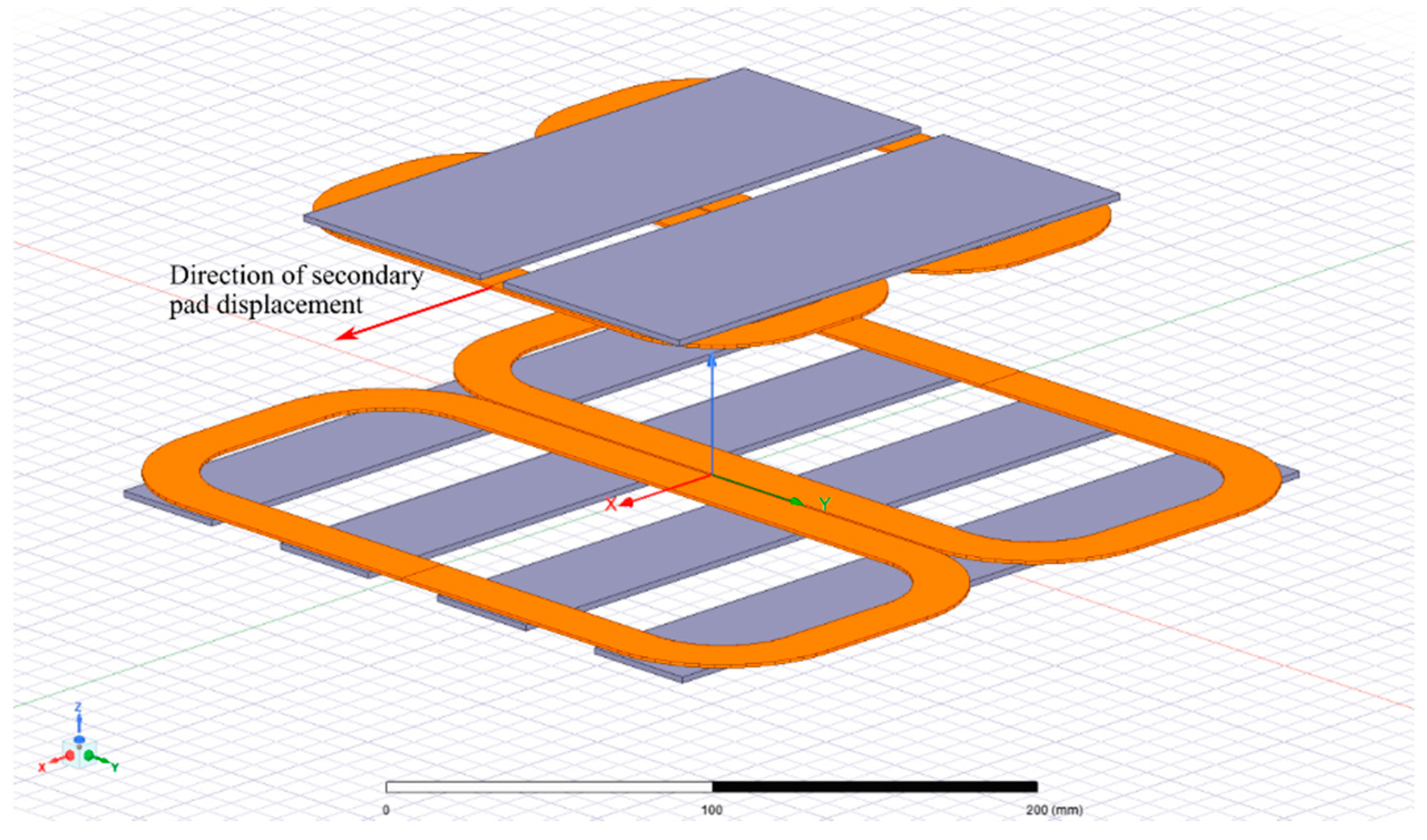
The presented method is evaluated together with selected existing methods by estimating the coupling coefficient $k$ during the secondary pad displacement. The secondary pad is horizontally moved in the x-axis (see Figure 6) in 10 mm steps from the initial position of 0 to 200 mm. The step is decreased to 5 mm near the DD pads null position (see Figure 9c in [15]).

Figure 6. Secondary pad displacement in x axis.

The coupling coefficient values used as a reference for method evaluation were measured by the following procedure using the calibrated LRC bridge.

(1)

Both pads are disconnected from the rest of the circuit.

(2)

The primary coil inductance $L_{1a}$ is measured while the secondary coil is open.

(3)

The secondary coil is short circuited. The primary inductance is measured again and labeled as $L_{1b}$. $L_{1b}$ is related to $L_{1a}$ via:

$$L_{1b}=L_{1a}\left(1-k^2\right)$$

(17)

(4)

The coupling coefficient $k$ is then calculated from (17) as:

$$k=\sqrt{1-\frac{L_{1b}}{L_{1a}}}$$

(18)

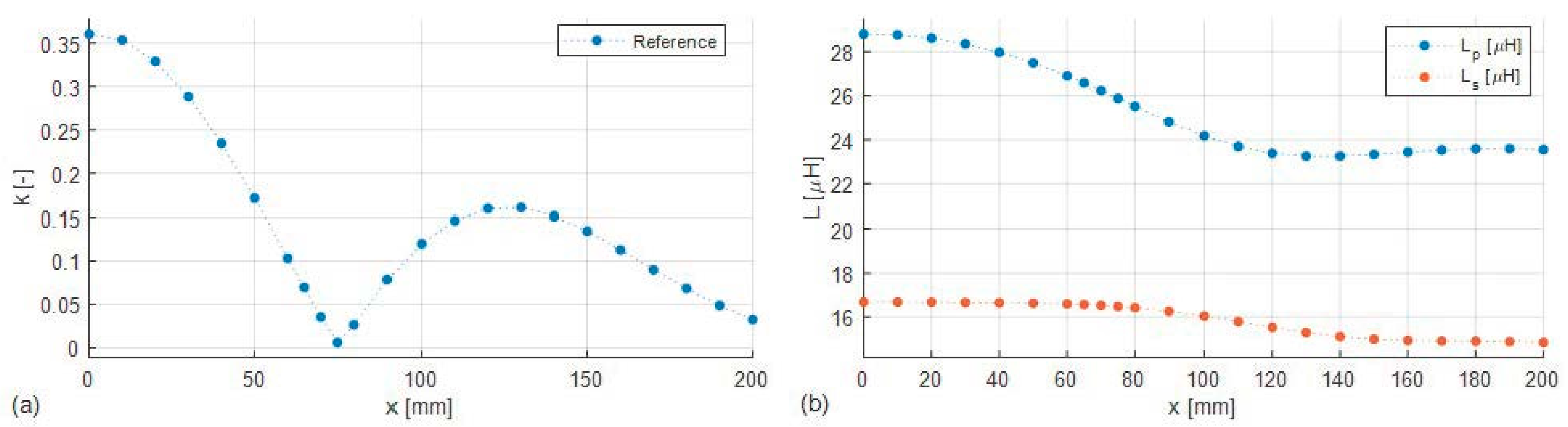
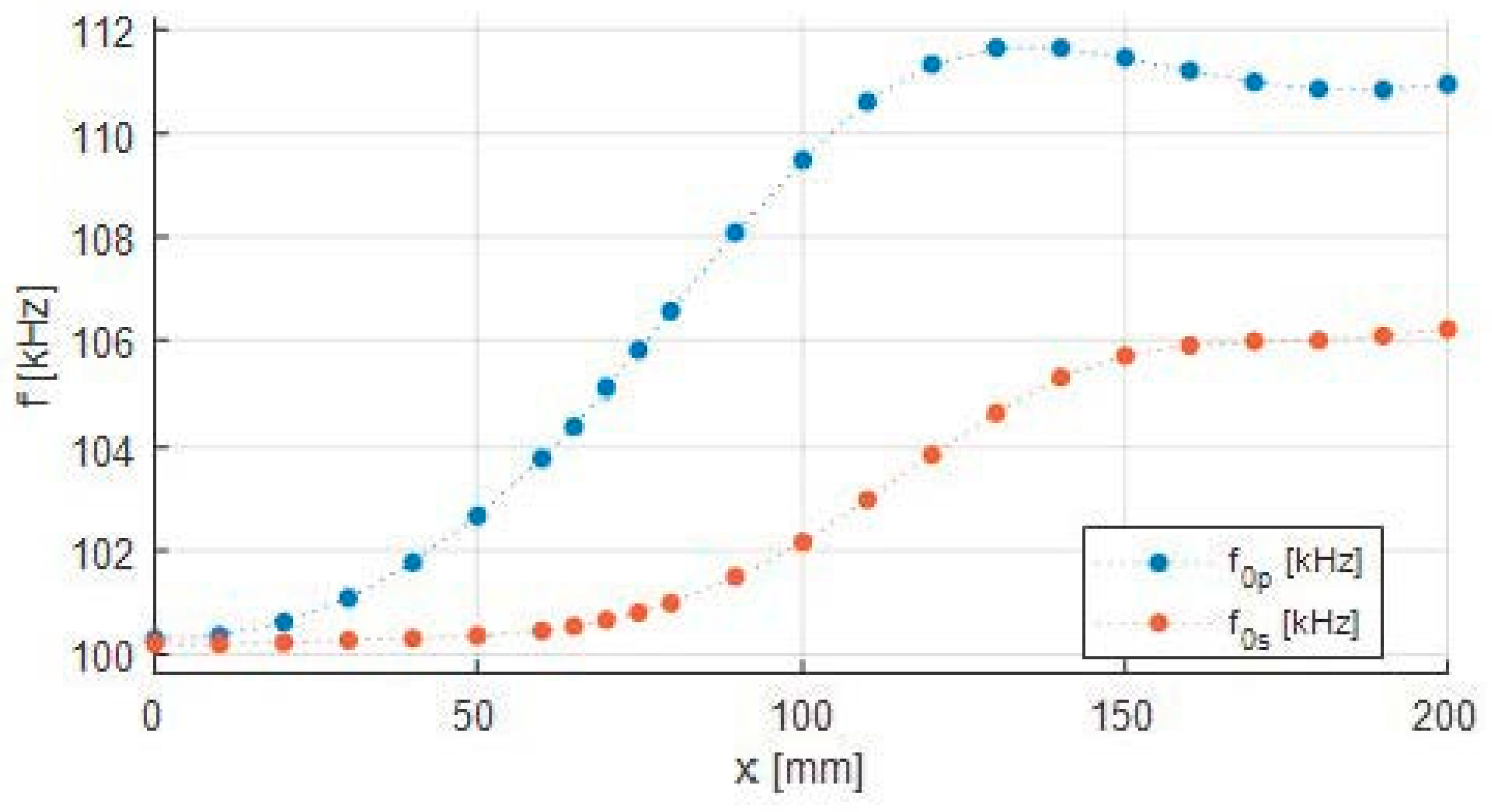
Figure 7 depicts the resulting $k$ values (a) together with the primary and secondary inductances $L_1$ and $L_2$ (b). The figure clearly shows the null point of the DD pads near x = 75 mm. The resulting sequence of $k$ covers the interval of 0.08 to 0.35, which is an aggregated range of $k$, which the IPT systems presented in SAE J2954 as examples for EV stationary charging gain under displacement [10]. As Figure 7b shows, the movement of the secondary coil changes the coil inductances, which in turn detunes the primary and secondary circuits. The impacts of detuning will be discussed for each method individually.

Figure 7. Reference values for x-axis displacement. (a) Coupling coefficient k. (b) The primary and secondary inductances L₁ and L₂.

The methods for estimating $k$ are compared with the reference measurement presented in Figure 7a. For each displacement position, the relative error with respect to the reference value is calculated according to:

$$\Delta k_r=\frac{k_M-k_{ref}}{k_{ref}}[\%]$$

(19)

where $k_M$ is the value estimated by the method and $k_{ref}$ is the reference value.

5.3. Bifurcation Asymptotes Method

The proposed method for estimating $k$ was implemented and tested according to the procedure outlined in Section 4. The method employed the setup shown in Figure 5, only the load was short-circuited at its connection point at the secondary switchboard. For each displacement position, the input current amplitude $I_{in}$ was measured with a step size of 1 kHz to find the approximate values of $f_{1a}$ and $f_{2a}$. These were then refined by measurement of the input phase ${\phi }_{in}$ measured with a step size of 0.5 kHz in interval ±1 kHz around the previously approximated frequencies $f_{1a}$ and $f_{2a}$, and consequent linear interpolation. 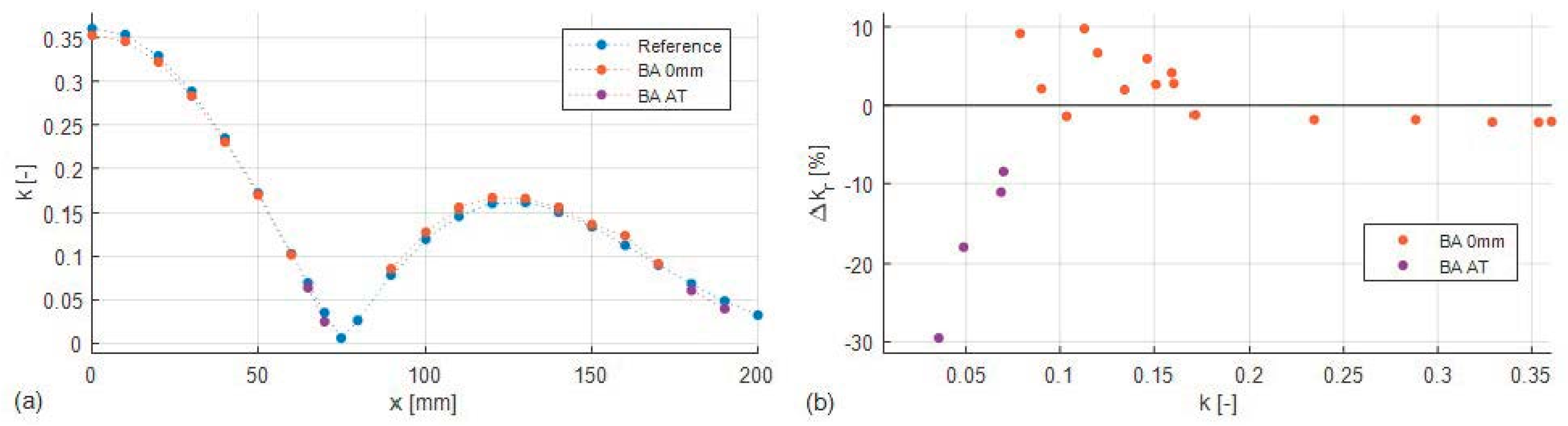The obtained estimates of $k$ “BA 0 mm” and “BA AT” are compared in Figure 8a with the reference “ref”. Label “BA 0 mm” marks the measurement with the system tuned to $f_0=$ 100 kHz in the initial position x = 0 mm and “BA AT” refers to the measurement when the system was manually tuned by adjusting the primary and secondary capacitances for each misalignment position to $f_0=$ 100 kHz (AT stands for always tuned).

Figure 8. Bifurcation asymptotes method. (a) Comparison with the reference measurement. (b) Relative error with respect to the reference over k. “BA 0 mm” refers to system tuned for x = 0 mm. “BA AT” refers to system tuned for each misalignment position.

For the system tuned at x = 0 mm, the method works well until approximately $k$ = 0.17, as it has a relative error of approximately −2% (see Figure 8b), which is calculated according to (19). The negative sign means that the method underestimates $k$ in comparison with the reference.

As $k$ decreases less than $k=$ 0.17, the relative error becomes positive, and its value increases up to 10%. For $k$ smaller than approximately 0.08, the method fails altogether. However, for most practical systems [10], k is larger than 0.08 (typically, k > 0.2 is expected for high efficiency) so the method’s breakdown at low values of k is not expected to pose a limitation in practice.

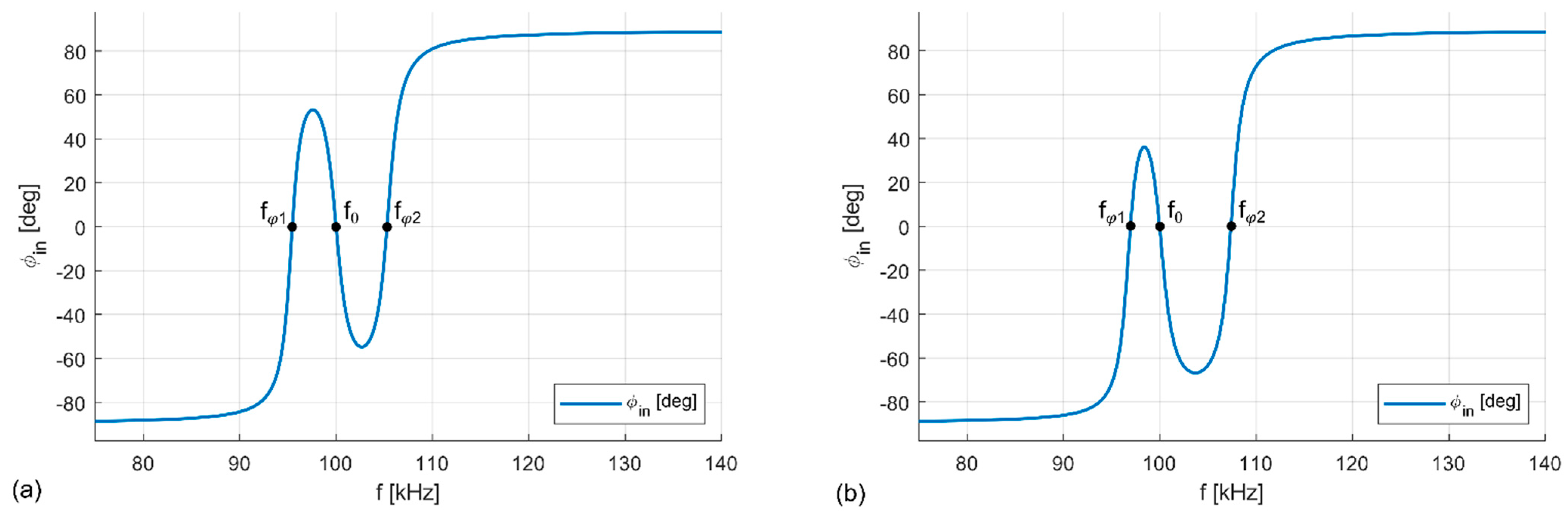
The increase of the relative error for $k$ below 0.17 and the method’s failure for $k$ lower than 0.08 is primarily caused by detuning. Figure 9 shows that with increasing displacement the primary resonance frequency $f_{0p}$ increases above the secondary resonance frequency $f_{0s}$. This detuning alters the frequency response of ${\phi }_{in}$. Because $f_{0p}>f_{0s}$, the frequency response moves below zero in comparison with the case $f_{0p}=f_{0s}$—see Figure 10a for the tuned system and Figure 10b for the detuned system.

Figure 9. Detuning of the primary and secondary side.

Figure 10. Frequency response shift due to detuning, illustrated on the displacement position of x = 60 mm. (a) Both sides are tuned to f₀ = 100 kHz. (b) The side resonance frequencies are given by Figure 9, i.e., f_0p = 103.27 kHz and f_0s = 100.13 kHz.

Under the displacement, the frequency responses change both with detuning and with changing $k$, as illustrated in Figure 11. In deep bifurcation, the frequency response of ${\phi }_{in}$ is relatively sharp near the zero crossings and it approaches its limiting values of −90° and +90° between the crossings if $k$ is sufficiently high (see Figure 11a,b). Thus, the impacts of detuning are smaller for high $k$, as even with the shift the frequency response resembles a straight line at the zero crossing and can be approximated as a linear function there (see Figure 11b). However, as $k$ decreases due to displacement, the frequency response curve becomes less pronounced, and it begins to cross zero near its peak, where it does not resemble a straight line (see Figure 11c). This increases the relative error. With a further decrease of $k$ and increase of detuning, former zero crossings are shifted below zero and only a single zero crossing occurs—Figure 11d. Thus, for low $k$ and increased detuning, the method fails.

Figure 11. Influence of detuning on the bifurcation asymptote method. (a) Tuned system (x = 0 mm). (b) Detuned system with medium coupling coefficient k (x = 130 mm). (c) Detuned system with small k (x = 60 mm). (d) Detuned system with very small k (x = 180 mm). The discrepancies between the measured data points and calculated frequency response (especially in (d)) are caused by high sensitivity of frequency responses for low k and the influence of the ferrites.

The method’s performance for low $k$ can be improved by maintaining the tuned system for specific inductance values under displacement by adjusting the primary and secondary compensation capacitances. The compensation adjustment can be done by e.g., switched capacity, or manually, as in our case. By removing the detuning, it was possible to obtain an approximate value of $k$ in positions 65, 70, 180, and 190 mm—see “BA AT” in Figure 8a. However, even though as $k$ decreases the measurement error grows up to 30%, as shown in Figure 8b. The high error is caused by the fact that the bifurcation is not deep enough such that frequencies $f_{\phi 1}$ and $f_{\phi 2}$ are not adequately meeting their asymptotes $f_{1a}$ and $f_{2a}$, respectively. After $k$ decreases under 0.04, not even tuning for a specific displacement position could help to achieve any meaningful results.

In the remaining points (75, 80, and 200 mm), only one zero crossing of the input phase was measured, even when the measurement step was decreased to 0.25 kHz. This may be caused either because the lack of bifurcation or the measurement step is still too coarse.

In applying the bifurcation asymptotes method, it is necessary to consider the impacts of the bifurcation phenomena on the input impedance $\widehat{Z}$. When short-circuiting the output, the input impedance is relatively high at $f_0$ (e.g., $Z=99.3$ Ω for x = 0 mm). However, near the ZPA frequencies $f_{\phi 1}$ and $f_{\phi 2}$ the impedance is very low (e.g., $Z=0.73$ Ω), which is determined by the ESRs $R_p$ and $R_s$. Thus, to limit the currents to 5 to 7 A in the primary side corresponding with the regular operation, the input voltage $V_{in}$ was decreased to 5 V when applying the method.

5.4. Faraday’s Law Method

For comparison, we consider another common approach for extracting $k$ by directly measuring the induced EMF in the secondary coil and solving for $M$ using Faraday’s law of electromagnetic induction. The adjusted measurement setup is depicted in Figure 12. Both pads are placed in their positions. The secondary coil is open, and the primary coil is in series with a resistor and a capacitor, which provide control of the coil current $I_1$. The primary coil current was limited between 5.8 and 6.6 A during the measurement process.

Figure 12. Faraday’s law method for measurement setup.

The primary coil is excited with current $I_1$, which is measured with a precision current shunt. The $I_1$ value is controlled with a resistor and a capacitor, which reduces the inductive character. The value of $I_1$ is adjusted to equal the value of $I_{in}$ during regular operation, to consider ferrite saturation and similar effects. The voltage $V_2$ is measured across the secondary coil terminals, and the mutual inductance $M$ is calculated as:

$$M=\frac{V_2}{\omega I_1}$$

(20)

The coupling coefficient $k$ is calculated from $M$ and the measured coil inductances $L_1$, $L_2$ according to (12).

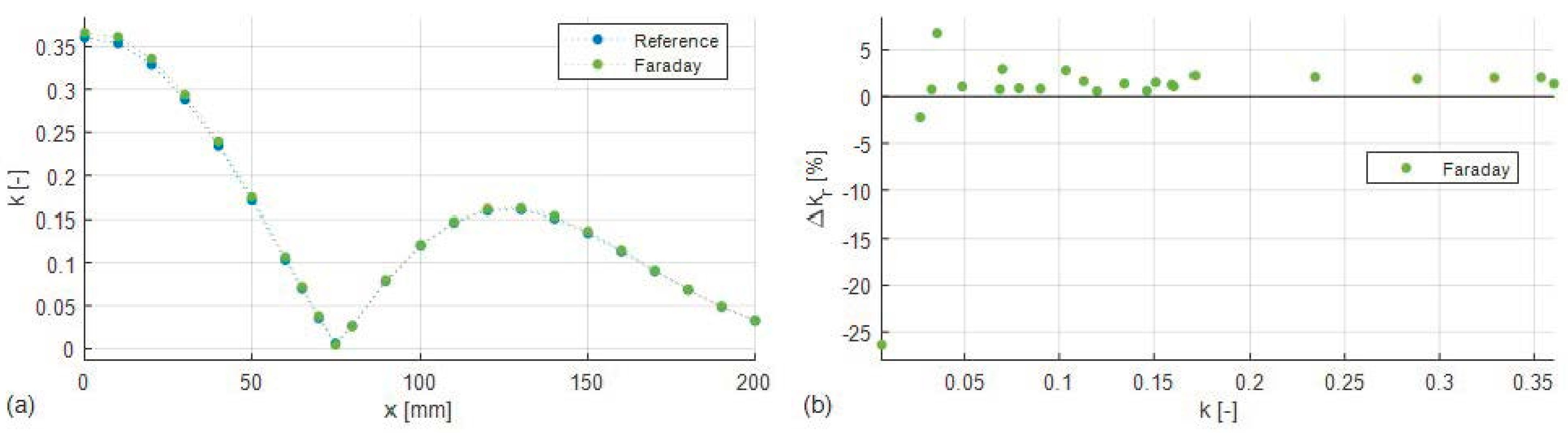
The estimated values of $k$ obtained by Faraday’s law method are compared with the reference measurements in Figure 13a. The relative error depicted in Figure 13b is very low even for low $k$ values. The distribution of error shows that the method generally estimates $k$ approximately by 1.55% above the reference. Faraday’s law method is unaffected by detuning.

Figure 13. Method based on Faraday’s law. (a) Comparison with the reference measurement. (b) Relative error with respect to the reference over k.

5.5. Method of Jiwariyavej

The second method used for comparison was presented by Jiwariyavej et al. in [18]. The variant for a single receiver was used. This method does not directly measure $k$ but the mutual inductance $M$. The calculation of $M$ is based on the equation for the real part of input impedance:

$$Re\left\{\widehat{Z}\right\}=R_p+{\left(\omega M\right)}^2\frac{R_L+R_s}{{\left(R_L+R_s\right)}^2+X_s^2}$$

(21)

where $X_s$ is the secondary side reactance:

$$X_s=\omega L_s-\frac{1}{\omega C_s}$$

(22)

The mutual inductance $M$ is then calculated as:

$$M=\frac{1}{\omega }\sqrt{\frac{\left(Re\left\{Z_{in}\right\}-R_p\right)\left({\left(R_L+R_s\right)}^2+X_s^2\right)}{R_L+R_s}}$$

(23)

The real part of input impedance $Re\left\{Z_{in}\right\}$ is calculated from the input current and voltage amplitudes $I_{in}$ and $V_{in}$, respectively, and the input phase:

$$Re\left\{Z_{in}\right\}=\frac{V_{in}}{I_{in}}cos{\phi }_{in}$$

(24)

The coupling coefficient $k$ is then calculated according to (12). Obtaining the value of $k$ according to this method requires preliminary measurement of $R_L$, $R_p$, $R_s$, $L_p$, $L_s$, and $C_s$.

The method was tested using the measurement setup shown in Figure 5, with the resistive load set to 31.8 Ω. Due to the higher number of preliminary parameter measurements, the method was measured in reduced number of points. The primary and secondary capacitances were adjusted to keep the system tuned at resonance frequency $f_0=$ 100 kHz against variations in coil inductance; see the illustration in Figure 7b. The specific values of the circuit parameters measured for each displacement position were used to calculate $M$ according to (23) and consequently $k$ according to (12).

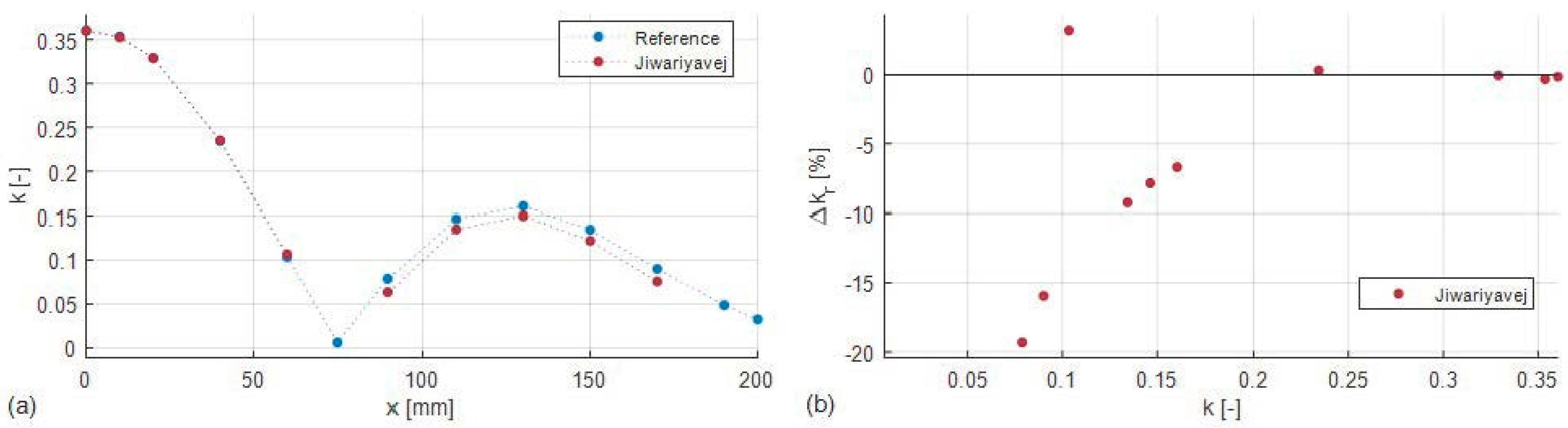
Values of $k$ obtained using the method of Jiwariyavej are compared to the reference values in Figure 14a. In addition to the plotted values, the method was also applied at displacement of 75, 190, and 200 mm, but did not provide any useful results. Thus, despite tuning for each displacement position, the method of Jiwariyavej suffers a similar limitation for small values of $k$ as the bifurcation asymptote method, which was tuned only for x = 0 mm.

Figure 14. Method presented by Jiwariyavej in [18]. (a) Comparison with the reference measurement. (b) Relative error with respect to the reference over k.

The relative error of the method of Jiwariyavej is depicted in Figure 14b. For high $k$ values (above approximately 0.23), this method exhibits good agreement with the reference. On the other hand, as $k$ is decreased, the error grows significantly and reaches 19.3% at $k=$ 0.08.

5.6. Measurement Comparison

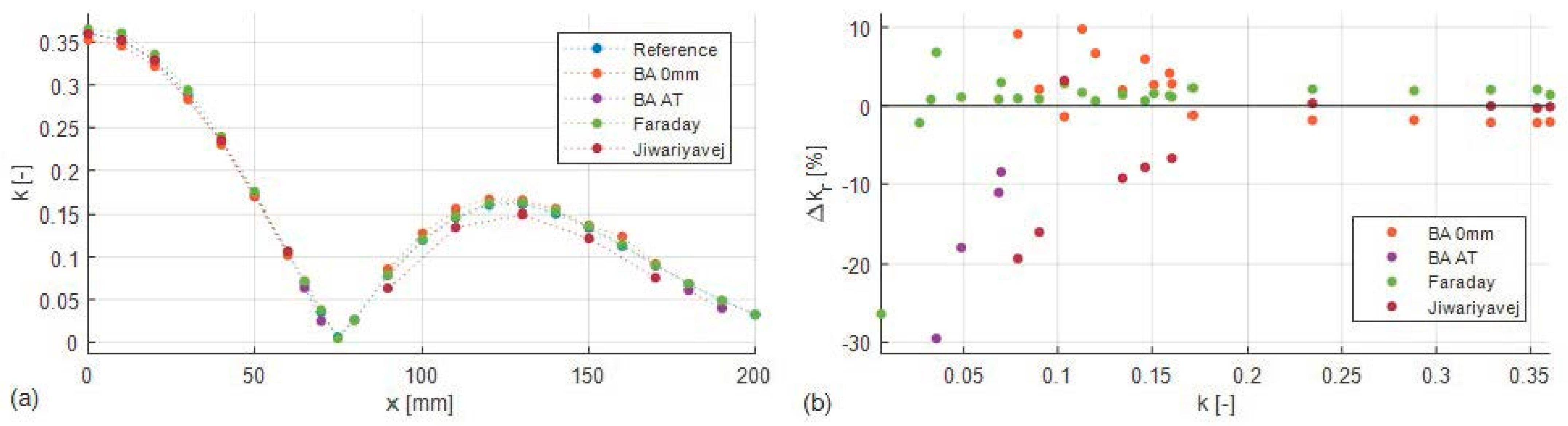
A comparative evaluation of the methods for estimating k is summarized in Figure 15. Figure 15a shows how the methods compare directly to the reference and Figure 15b shows their relative errors.

Figure 15. (a) Comparison of all tested estimation methods with the reference. (b) Relative error of the estimation methods with respect to the reference over k.

The evaluation of the methods is divided in two intervals $k\in ⟨0.08,0.23⟩$ and $k\in ⟨0.23,0.36⟩$ based on the relative error results shown in Figure 15b. The bottom limit of $k=0.08$ was selected as the final value, at which point all three methods yielded a result. Thus, only the bifurcation asymptote method with tuning at x = 0 mm was evaluated. For each interval, the method is evaluated based on the average error ${\overline{\Delta k}}_r$ and average absolute error $\left|{\overline{\Delta k}}_r\right|$, which are calculated as:

$${\overline{\Delta k}}_r=\frac{1}{n_M}{\displaystyle \sum }_{i=1}^{n_M}\Delta k_{r,i}=\frac{1}{n_M}{\displaystyle \sum }_{i=1}^{n_M}\frac{k_{M,i}-k_{ref,i}}{k_{ref,i}}[\%]$$

(25)

$${\overline{\Delta k}}_r=\frac{1}{n_M}{\displaystyle \sum }_{i=1}^{n_M}\left|\Delta k_{r,i}\right|=\frac{1}{n_M}{\displaystyle \sum }_{i=1}^{n_M}\frac{\left|k_{M,i}-k_{ref,i}\right|}{k_{ref,i}}[\%]$$

(26)

while $\left|{\overline{\Delta k}}_r\right|$ quantifies the disagreement between the method’s results from the reference in the selected interval. ${\overline{\Delta k}}_r$ describes the shift of the estimate with respect to the reference, i.e., if ${\overline{\Delta k}}_r\to 0$ then the values are distributed evenly around the reference. The results are summarized in Table 2.

Table 2. Overview of the average relative errors ${\overline{\Delta k}}_r$ and average absolute errors $\left|{\overline{\Delta k}}_r\right|$ of the evaluated methods.

Method	$$\mathit{k}\in ⟨0.08,0.23⟩$$	$$\mathit{k}\in ⟨0.23,0.36⟩$$	$$\mathit{k}\in ⟨0.08,0.36⟩$$
Bifurcation asymptote method	$$\begin{gathered} {\overline{\Delta k}}_r=3.87\% \\ \left|{\overline{\Delta k}}_r\right|=4.36\% \end{gathered}$$	$$\begin{gathered} {\overline{\Delta k}}_r=-2.01\% \\ \left|{\overline{\Delta k}}_r\right|=2.01\% \end{gathered}$$	$$\begin{gathered} {\overline{\Delta k}}_r=2.04\% \\ \left|{\overline{\Delta k}}_r\right|=3.62\% \end{gathered}$$
Faraday’s law method	$$\begin{gathered} {\overline{\Delta k}}_r=1.39\% \\ \left|{\overline{\Delta k}}_r\right|=1.39\% \end{gathered}$$	$$\begin{gathered} {\overline{\Delta k}}_r=1.91\% \\ \left|{\overline{\Delta k}}_r\right|=1.91\% \end{gathered}$$	$$\begin{gathered} {\overline{\Delta k}}_r=1.55\% \\ \left|{\overline{\Delta k}}_r\right|=1.55\% \end{gathered}$$
Jiwariyavej’s method	$$\begin{gathered} {\overline{\Delta k}}_r=-9.30\% \\ \left|{\overline{\Delta k}}_r\right|=10.38\% \end{gathered}$$	$$\begin{gathered} {\overline{\Delta k}}_r=-0.04\% \\ \left|{\overline{\Delta k}}_r\right|=0.20\% \end{gathered}$$	$$\begin{gathered} {\overline{\Delta k}}_r=-5.6\% \\ \left|{\overline{\Delta k}}_r\right|=6.31\% \end{gathered}$$

All three estimation methods show a good match to the reference for $k$ above 0.23. From these values it is evident that the Jiwariyavej’s method exhibits the best match to the reference ($\left|{\overline{\Delta k}}_r\right|=0.20$%), with the estimates which are distributed evenly around the reference (${\overline{\Delta k}}_r=-0.04$%). The estimates of the method based on Faraday’s law are shifted above the reference (${\overline{\Delta k}}_r=1.91$%), while the estimates of the bifurcation asymptotes method are shifted below the reference (${\overline{\Delta k}}_r=-2.01$%).

However, with decreasing $k$ all methods except Faraday’s law method decrease in precision (interval $k\in ⟨0.08,0.23⟩$). Faraday’s law method is the most accurate ($\left|{\overline{\Delta k}}_r\right|=1.39$%), but its estimates are again shifted above the reference (${\overline{\Delta k}}_r=1.39$%). The second-best method is the bifurcation asymptotes method ($\left|{\overline{\Delta k}}_r\right|=4.36$%) which is now shifted above the reference (${\overline{\Delta k}}_r=3.87$%). The Jiwariyavej’s method performs much worse ($\left|{\overline{\Delta k}}_r\right|=10.38$%) and its value begins to move further below the reference with decreasing $k$—see Figure 15b, ${\overline{\Delta k}}_r=-9.30$%.

Across the whole measured interval of $k\in ⟨0.08,0.36⟩$, Faraday’s law method is the most accurate ($\left|{\overline{\Delta k}}_r\right|=1.55$%), followed by the bifurcation asymptote method ($\left|{\overline{\Delta k}}_r\right|=3.62$%) and then Jiwariyavej’s method ($\left|{\overline{\Delta k}}_r\right|=6.31$%). The estimates of the two first methods are on average shifted above the reference ($\left|{\overline{\Delta k}}_r\right|=1.55$% and $\left|{\overline{\Delta k}}_r\right|=3.62$%, respectively), while the third is shifted below the reference (${\overline{\Delta k}}_r=-5.6$%).

The shifts of the estimates with respect to the reference could be partially explained by the different measurement currents used in each method (see Table 3) and the reference, which was measured with the LRC meter and thus with very small currents. The high currents could result in detuning caused by the dependance of the coil inductances on the currents through the coils and ferrite non-linearity [27], as the ferrites are used as the magnetic cores of the DD pads. This effect could especially impact the Jiwariyavej’s method, as the primary currents were significantly higher in the second interval.

Table 3. Currents used for testing of the estimation methods.

Method	${\mathit{I}}_{\mathit{i}\mathit{n}}$	${\mathit{I}}_{\mathit{o}\mathit{u}\mathit{t}}$
Bifurcation asymptote method	5 to 7 A	5 to 10 A
Faraday’s law method	5 to 7 A	Open
Jiwariyavej’s method	$4.5 \mathrm{to} 6 \mathrm{A} (k\in ⟨0.23,0.36⟩)$ $10.5 \mathrm{A} (k\in ⟨0.08,0.23⟩)$	$0.5 \mathrm{to} 1 \mathrm{A} (k\in ⟨0.23,0.36⟩)$ $0.5 \mathrm{A} (k\in ⟨0.08,0.23⟩)$

Some of the differences could also be explained as a result of measurement errors due to limited instrument accuracy, loading effects, and environmental factors such as temperature, etc.

6. Discussion

As evaluated in the previous chapter, the bifurcation asymptote method provides relatively accurate estimates ($\left|{\overline{\Delta k}}_r\right|=3.62$%) across the interval of $k\in ⟨0.08,0.36⟩$. However, the estimate precision is not the only consideration for evaluating the usability of the method. Table 4 summarizes some of the practical aspects of all three evaluated methods, which should also be considered.

Table 4. Comparison of the practical aspects of the bifurcation asymptotes method with the selected estimation methods.

Method	Bifurcation Asymptotes Method	Faraday’s Law Method	Jiwariyavej’s Method [18]
Measured parameter	$k$	$M$	$M$
Use during operation	Intermittent	No	Yes, but only for air-core coils
Required active measurements	$f$$, {\phi }_{in}$$, I_{in}$ (optional)	$f$$, I_1$$(\mathrm{primary} \mathrm{coil} \mathrm{current} \mathrm{amplitude}), V_2$ (secondary coil voltage amplitude)	$f$$, I_{in}$$, V_{in}$$, {\phi }_{in}$
Number of frequency points required	$\mathrm{Varies} \mathrm{with} k$	1	1
Required preliminary measurements	None $(\mathrm{general} \mathrm{knowledge} \mathrm{of} f_0$ to specify measurement range)	$\mathrm{None} \mathrm{to} \mathrm{obtain} M$, $L_p$$, L_s$$\mathrm{to} \mathrm{obtain} k$	$R_L$$, R_p$$, R_s$$, L_s$$, \mathrm{and} C_s$$\mathrm{to} \mathrm{obtain} M$, $\mathrm{plus} L_p$$\mathrm{to} \mathrm{obtain} k$
Other requirements	Ability to short-circuit the load. Source with variable frequency Decreased source voltage	Open secondary coil	$\mathrm{Air}-\mathrm{core} \mathrm{coils}, \mathrm{or} L_p$$\mathrm{and} L_s$ must be remeasured after displacement

While the method based on Faraday’s law provides very accurate estimates, it requires the ability to disconnect the secondary coil from the rest of the circuit and measure the coil voltage across its open terminals. Thus, this method is more suitable for characterizing the coils in the laboratory setting than performing real-time estimations of $k$ for practical applications such as EV charging.

Jiwariyavej’s method for a single receiver also provides accurate estimates, but only for higher $k$ values: $k\in ⟨0.08,0.36⟩$. Another disadvantage is that it requires additional preliminary measurements including $L_s$ to calculate the value of $M$. Due to this, use of Jiwariyavej’s method during operation is limited to air-core coils in which the inductance does not vary with displacement. The method is not very useful for the coils with magnetic cores, as their inductances change with displacement.

The main downside of the bifurcation asymptotes method is that it requires short- circuiting of the load; therefore, it cannot provide estimation of $k$ during the operation of an IPT system. However, the method can be used to estimate k intermittently during a charging cycle and at critical times such as at start-up. In addition, the method involves measuring the frequency response; thus, a variable frequency source is required, and a certain amount of time given by transients must be allotted for the extraction process to occur.

In return, however, the bifurcation asymptotes method provides significant advantages. Namely, the method requires no a-priori information of the system component values, it is based purely on primary-side measurements, it estimates $k$ with good accuracy ($\left|{\overline{\Delta k}}_r\right|=3.62$% for $k\in ⟨0.08,0.36⟩$), and it is resilient to the detuning caused by the displacement of the coils with magnetic cores. Thanks to this, the bifurcation asymptotes method presents an interesting option for estimating $k$ that can be readily employed by control strategies that require an accurate estimation of this variable. The method is especially suitable for implementation at the startup of stationary charging applications. For example, the method can be used to estimate $k$ immediately after an EV is parked over a stationary wireless charger to determine if the EV is suitably positioned to allow for efficient wireless charging before high power is applied to the primary.

7. Conclusions

This paper presented a novel bifurcation asymptotes method for accurately estimating the coupling coefficient $k$ for SS compensated IPT systems. The method involves temporarily operating the system in bifurcation by short-circuiting the load and measuring the zero phase angle frequencies at the primary. The method can be used by control algorithms that require the value of $k$, and is especially suitable for implementation at the startup of certain applications such as EV stationary charging. This paper presents a preliminary evaluation of the method, which contains the theoretical background and description of the method, experimental verification, and a comparison with existing $k$-estimation methods. The proposed method provides good estimates (average absolute error of $3.62$%) for a wide range of coupling coefficients ($k\in ⟨0.08,0.36⟩$).

For future work, we intend to evaluate the method performance in a non-idealized setup by implementing it in an inverter. We also intend to explore how this method can be extended to other compensation topologies such as series–parallel, LCC–series, etc. Finally, we intend to perform more comparisons with current $k$-estimation methods (e.g., [18,19] cited in the Introduction).