3D Face Recognition Based on an Attention Mechanism and Sparse Loss Function

Abstract

Face recognition is one of the essential applications in computer vision, while current face recognition technology is mainly based on 2D images without depth information, which are easily affected by illumination and facial expressions. This paper presents a fast face recognition algorithm combining 3D point cloud face data with deep learning, focusing on key part of face for recognition with an attention mechanism, and reducing the coding space by the sparse loss function. First, an attention mechanism-based convolutional neural network was constructed to extract facial features to avoid expressions and illumination interference. Second, a Siamese network was trained with a sparse loss function to minimize the face coding space and enhance the separability of the face features. With the FRGC face dataset, the experimental results show that the proposed method could achieve the recognition accuracy of 95.33%.

1. Introduction

Face recognition (FR) technology has been widely used in various public areas, such as railway stations, airports, supermarkets, campuses, and medicine [1,2]. Taking the advantage of noncontact recognition, FR has more applicability and better security with practical and commercial applications compared to traditional fingerprint, iris, and other biometric systems [3,4]. Extracting geometric features from faces combined with classifiers is a rudimentary FR method, including active appearance models (AAM) [5] and locality preserving projections (LPP) [6]. However, uncertainties of expressions often limit the recognition accuracy. The Local Binary Pattern (LBP) [7], Histograms of Oriented Gradients (HOGs) [8], and Gabor Wavelet Representation [9] were then proposed to extract appearance features. These features were used to be classified by a classifier, such as support vector machine (SVM) [10] or K-nearest Neighbors (KNN) [11]. However, the features designed manually could not describe exactly the characteristics of face, which limited the recognition accuracy.

Deep learning reconstructed the landscape of FR systems with the proposal of CNN. Ding [12] et al. proposed a video face recognition method, in which CNN was used as the backbone and branches to extract complementary information. Yang et al. [13] proposed a facial expression recognition method based on RI-LBP and ResNet to extract features using the extreme learning machine for classification. The experimental results showed that the proposed method could significantly improve the facial expression recognition accuracy, but the computational cost should be further reduced. Almabdy et al. [14] investigated the performance of pretrained CNN with multiclass SVM. These studies showed that CNN could extract features effectively for face recognition.

However, the current convolution module did not pay much attention to distinguishing parts of faces than other similar parts. It extracted not only useful features but also some redundant information as its output, so it could be improved by eliminating some useless parts for face recognition. The attention mechanism, as an emerging method in deep learning, could attend to specific parts of an image that are more important and informative [15]. This mechanism of attention mechanism simulated the attention and exception of the human visual system which helps our brain filter the observed scene to focus on its essential parts [16]. Li et al. [17] integrated an improved attention mechanism with the YOLOv3 and MobileNetv2 framework. Li et al. [18] proposed a novel end-to-end network with attention mechanism for automatic facial expression recognition. These studies showed that an attention mechanism was suitable for enhancing standard convolutional modules’ facial features extraction ability. Additionally, sparse representation was an effective way to build robust and small feature subspaces, and published works showed that sparse representation not only reduced the coding space of the feature but also improved the classification performance, which means that the sparsely represented features were more robust [19,20,21]. However, these research only focused on 2D images without depth information, which meant that the change in light or poses would affect the recognition accuracy.

With the development of three-dimensional scan devices [22], it has become a trend to build FR systems based on 3D data partly due to their illumination-invariant [23] expression-invariant [24] advantages. Lei et al. [25] presented a computationally efficient 3D face recognition system based on a novel facial signature called Angular Radial Signature (ARS) extracted from the semirigid region of the face. Liu et al. [26] proposed a joint face alignment and 3D face reconstruction method to reconstruct 3D faces to enhance face recognition accuracy. In order to improve recognition, self-attention [27] or data processing [28] was added into recognition network for point cloud recognition.

In this research, a 3D face scanning technique coupled with deep learning was used to solve the FR with a single face scan per person. The proposed algorithm integrated an improved CNN, which contained attention layers and the sparse loss function to build the FR model for a single scan per person. Different from the classic CNN architecture, in the attentive CNN, the output of CNN was transferred to a corresponding attention map on the picture. Next, the advanced attention feature map from the attentive CNN was used as the input for a sparse representation network. Instead of using an end-to-end one branch network, the sparse representation network is constructed by two branches of network, which formed a Siamese network [29]. A Siamese network is a network with two branches that share the same network weight. Instead of using the Root Mean Squared Error or Crossentropy as loss function, the proposed Siamese network used a distance-based sparse loss function in order to reduce the recoding size.

Specifically, the integrated model was used as the sparse representation transformer of 3D faces. Therefore, the specific objectives of the current research included the following:

• Develop a face recognition model based on 3D scan and deep learning for single 3D scan training data per person;
• Develop an attention layer to the classic CNN to compose ACNN to extract useful information based on the features of faces;
• Use a Siamese network structure to train the network with a sparse loss function to build a distance-based face feature transformer in order to avoid the impact caused by the small size of samples.

2. Materials and Methods

2.1. Introduction of Face Dataset and Preprocessing

The 3D face data with depth information used in this study were from the FRGC v2.0 Database [30] collected by the University of Notre Dame in the United States, including 4007 frontal face scan images of 466 individuals. The scanned images were collected using a 3D scanner in the autumn of 2003, spring of 2004, and autumn of 2004, including expressions such as expressionless, smiling, laughing, frowning, bulging, surprise, and small changes in attitude. This database was currently one of the most widely used benchmark datasets. 3D scanning data usually contained redundant data, including ears, hair, shoulders, and other areas that were not related to the human face. Furthermore, outliers that were spikes caused by collection equipment and environmental conditions were also included in the collected scan data, which were interference information for FR. Therefore, the 3D data in the FRGC v2.0 Database needed to be preprocessed.

First, outliers were eliminated, and the face position was corrected. In the obtained face data, the 3D information was recorded in the form of scattered points. Each data point represented the position of the 3D point achieved by the corresponding sensor. The 3D face data of a single face can be recorded as a point set ${\mathbb{P}}^n$, each point $p$ represents a measured point position vector. The position vector contains the measured three-axis information $\left[x, y, z\right]$ of the point. The utilized discrete point elimination method is as follows:

$$d\left(p_{i,j}\right) =\underset{\delta \in \left\{-1, 0, 1\right\}}{\max }\left|\left|p_{i,j}-p_{i+\delta ,j+\delta }\right|\right|$$

(1)

where $p_{i,j}$ represents the point at the $i$th row and $j$th column, $\delta$ means the index offset from $p_{i,j}$, and $d(p_{i,j})$ represents the maximum distance between $p_{i,j}$ and the adjacent designated area point. The outlier points would be filtered out by setting the threshold $d_s$ for this distance, and the threshold $d_s$ is defined as follows:

$$d_s=\mu +c\sigma$$

(2)

$$\mu =\frac{1}{n}{\displaystyle \sum }_{p_{i,j}\in \mathbb{P}}d(p_{i,j})$$

(3)

$$\sigma =\sqrt{\frac{1}{n}{\displaystyle \sum }_{p_{i,j}\in \mathbb{P}}{(d\left(p_{i,j}\right)-\mu )}^2}$$

(4)

where $\mu$ is the average sample distance of each collected face data $\mathbb{P}$, $\sigma$ is the sample variance of each face sample data $\mathbb{P}$, $c$ is the threshold hyperparameter for face outlier segmentation, and $d_s$ is the threshold for outlier judgment. In this research, the segmentation threshold hyperparameter c was set as 0.6 according to the literature [31] to complete the elimination of outliers.

After eliminating outliers, the Shape Index (S.I.) [32] was used to locate the nose point for face alignment. Different shape index values corresponded to different curved surface shapes. The more concave curved surface had a smaller shape index, and the more prominent curved surface had a larger shape index.

When the shape index was close to 1, the curved surface was closer to the hemispherical hat-shaped surface, and is more similar to the shape of the nose tip in the face. Therefore, the connected domain composed of points greater than 0.85 was selected to be the nose tip candidate region ${ℝ}_1$; then the 3D point cloud was calculated. Taking the center of mass as the sphere and the spherical area with radius $r=5 \mathrm{mm}$ as the candidate area ${ℝ}_2$, the candidate area of the nose point was ${ℝ}_{nose}={ℝ}_1\cap {ℝ}_2$, and the nose point used the point with the largest z value in the candidate area of the nose point, that is, the nose point $p_{nose}=\underset{\mathrm{z}}{\max }{R}_{nose}$. After calculating the confirmed nose tip point by this formula, the nose tip point could be the center of the circle, and the radius of $90 \mathrm{mm}$ could be used as a ball to cut the point cloud. The point cloud obtained at this time was the desired face area.

After obtaining the face area data, the cubic interpolation operation [33] was performed to smooth the face area. Then it was projected onto a two-dimensional plane to form a grayscale image for subsequent use. The above point cloud data preprocessing steps can be summarized as follows:

• Step 1: Use Equation (1) to calculate and count the corresponding parameters, eliminate outliers in the points set with Equation (2), and decrease the noise caused by the out-of-bounds environment.
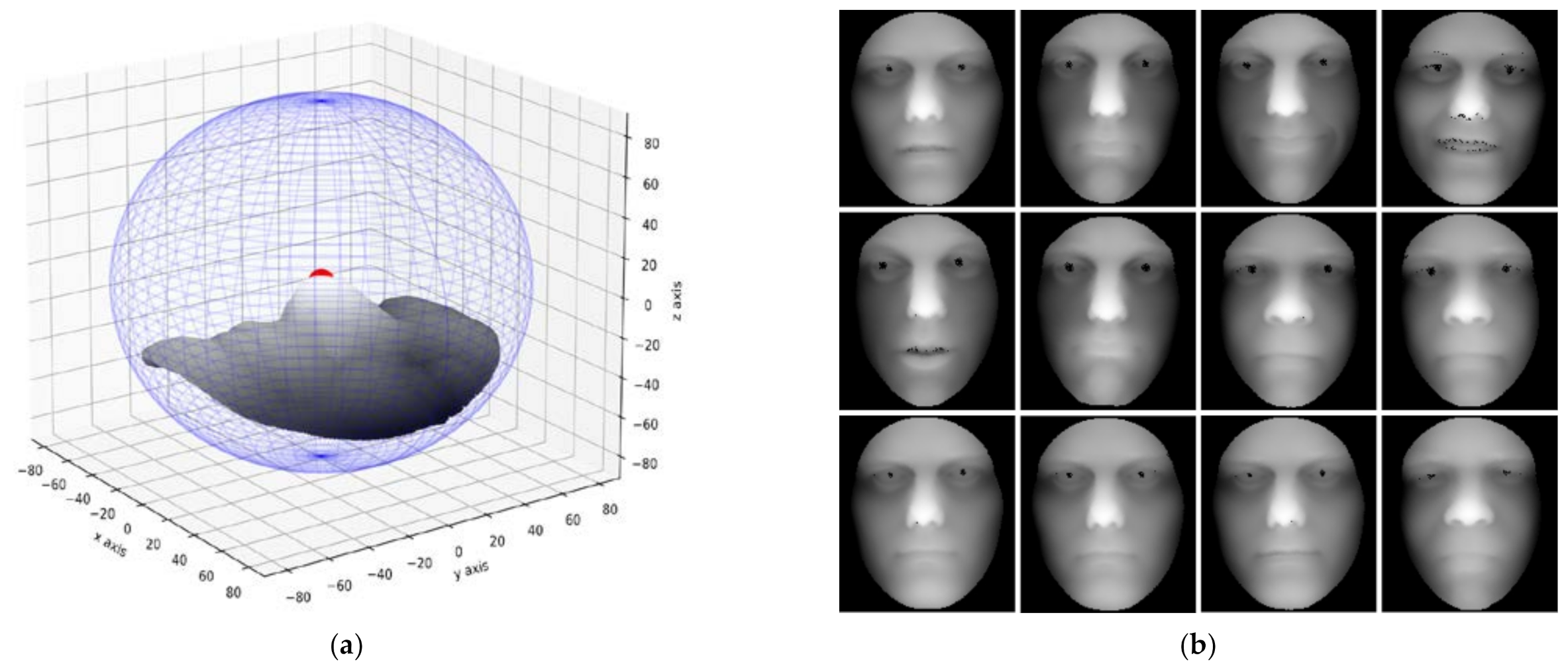
• Step 2: Use the S.I. to search the nose candidate area in the point cloud data and utilize the height of the z-axis to confirm the tip of the nose.
• Step 3: Use the tip of the nose found in step 2 to segment the point cloud data. The segmentation used the nose tip point as a sphere center and points in the spherical area with a radius of 90 mm were obtained as the face area.
• Step 4: Perform a bicubic interpolation operation on the obtained face area to achieve a smooth surface and the smoothed face area obtained is shown in Figure 1a.
• Step 5: Project the smoothed face surface onto a two-dimensional plane with the z-axis value to form a 2D grayscale image.

After completing the above steps, the preprocessed image will be a uniform face depth map, as shown in Figure 1b.

As shown in Figure 1, through the above conversion, the 3D point cloud data were transformed into a depth map of the face point cloud that was less affected by the environment illumination. The pixels’ gray value in the transformed image represented a distance from each point to the nose tip. The gray value of the area closer to the tip of the nose was high, and the gray value of the area farther from the tip of the nose was low.

2.2. 3D Face Recognition Based on Deep Learning

The process of the proposed face recognition algorithm is shown in Figure 2, and it included two main parts: (1) Training phase: the designed ACNN was used to construct a double branch Siamese network. The network was trained with a sparse loss function to obtain a sparse representation face coding space. (2) Testing phase: the face of a person was obtained and preprocessed and then, the trained network transformed it into a sparse face coding space for face matching.

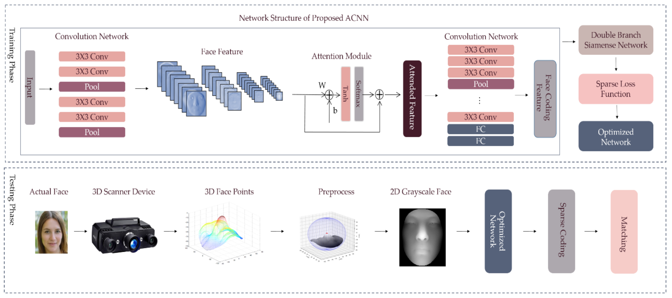
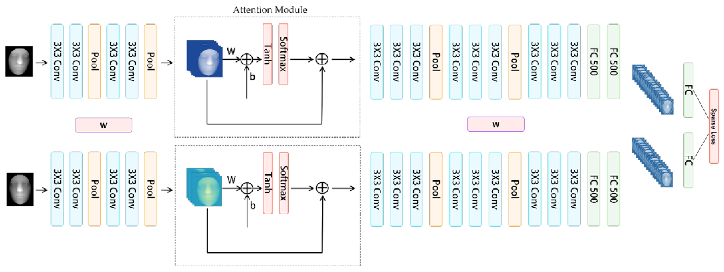
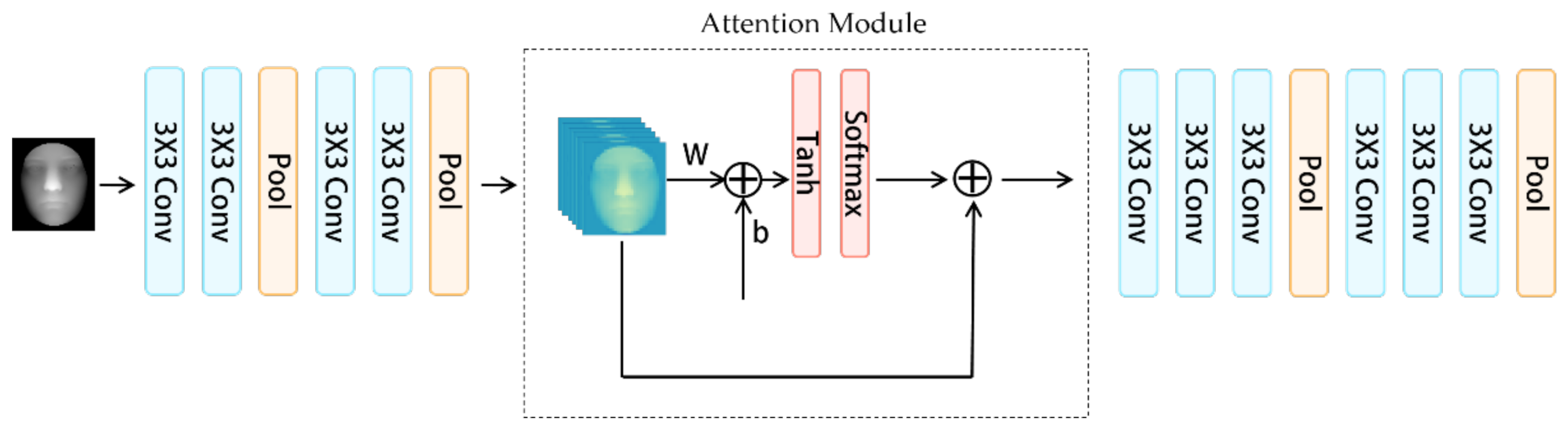
2.2.1. Face Feature Extracting Module based on Attention Mechanism and Convolutional Layers

Face detection is based on vision target detection, and it is essential to find the key points or critical areas of the face as a basis for discrimination. Therefore, the attention mechanism coupled with the convolutional layers was constructed as the backbone network to focus on the key information of the preprocessed data in order to reduce the influence of different facial expressions on recognition accuracy.

The convolutional layer is known as a grid-like topological specialized kind of neural network which has gained tremendous success in practical applications [34,35]. This kind of neural network layer is able to extract robust features from images and is utilized as a feature extractor in this study. In order to enhance the ability of the feature extractor to eliminate the useless parts of the input, the attention mechanism was adopted as well.

The primary function of the attention mechanism is to use the image features as input to construct an attention map. Here, a spatial attention module was used, so the outputs of the former convolutional feature extraction module was used as the input of this one. The attention value is calculated as follows [36]:

$$y_a\left(i,j\right) = \mathrm{Softmax}\left(\tanh \left(W_{i,j}x\left(i,j\right) + b_{i,j}\right)\right)$$

(5)

$$Softmax\left(z_m\right) = \frac{e^{z_m}}{{\sum }_{k=1}^n{e}^{z_k}}$$

(6)

where $W$ is the set weight, $b$ is the set offset value, and $x\left(i,j\right)$ represents the value of the $\left(i,j\right)$ position in the last layer of the image after the feature extraction network. After the $\tanh$ function and the $\mathrm{softmax}$ function, the features selected in the previous step were processed for data.

Finally, the output $y_o\left(i,j\right)$ after the attention mechanism and the original image addition or multiplication operation was obtained by adding the original feature data after feature extraction and the data obtained by the attention mechanism as follows:

$$y_o\left(i,j\right) = y_{in}\left(i,j\right) + y_a\left(i,j\right)$$

(7)

where $y_{in}\left(i,j\right)$ represents the value of position $\left(i,j\right)$ in the original image feature, and $y_a\left(i,j\right)$ represents the output value of the attention mechanism module.

The feature processed by the attention mechanism can better reflect the local features of the face, which is of help for subsequent face recognition and classification. Figure 3 shows the structural diagram of the attention mechanism module coupled with the convolutional module. The input was the depth grayscale image obtained from the face 3D point cloud data preprocessing described in Section 2.1.

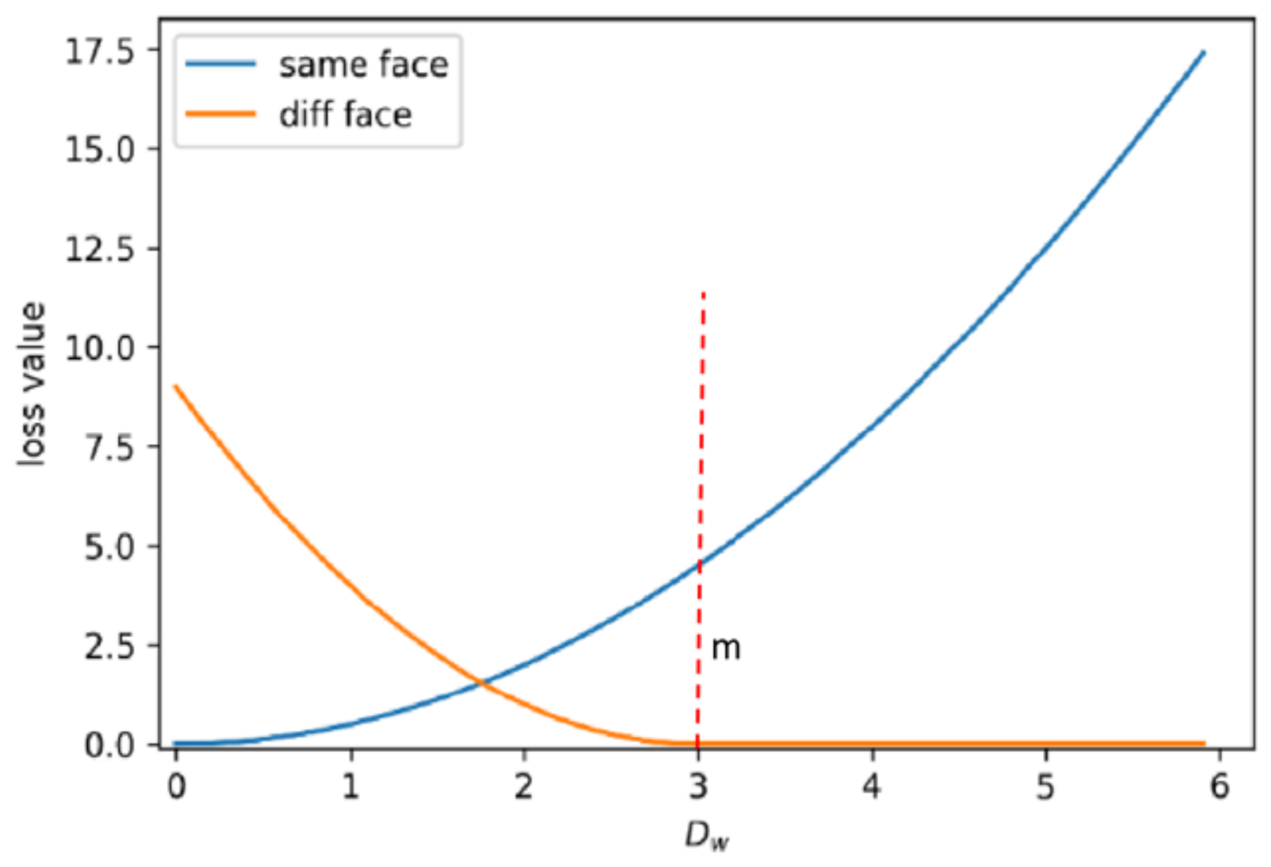
2.2.2. Siamese Network Trained with Sparse Contrastive Loss

The convolutional neural network coupled with the attention mechanism constructed in the previous section could effectively extract the face features, but as the number of categories increased the accuracy of the classification would show a downward trend as shown in Table 3 in the following Section 3.3. This section describes the form of a Siamese neural network to avoid the impact caused by the small size of samples with a single face scan per person. The network structure of the proposed method is shown in Figure 4. The largest difference between the Siamese neural network and the traditional convolutional neural network lies in two aspects. In terms of neural network structure, the Siamese neural network constructs two convolutional neural network branches in the form of weight sharing, and the two branches are used to extract the prediction results of two sets of data. In terms of the loss function, the Siamese neural network replaces the crossentropy function commonly used in classification problems through a unique distance measurement method, which improves the network’s interpretability and provides the neural network feature extraction training more in line with the difference extracting by changing the gradient direction.

The input size of the network was $128\times 128\times 1\left(width\times height\times channel\right)$ and the detailed parameters of the network are shown in

Table 1. Architecture parameters of the proposed ACNN.

Layer Type	Output Size	Branch1	Branch2
Conv	$64\times 128\times 128$	$3\times 3$, $64$, stride$1$	$3\times 3$, $64$, stride$1$
Conv	$64\times 64\times 64$	$3\times 3$, 64, stride $1$	$3\times 3$, 64, stride $1$
		$2\times 2$, Max pooling, stride $2$	$2\times 2$, Max pooling, stride $2$
Conv	$128\times 64\times 64$	$3\times 3$, 64, stride $1$	$3\times 3$, 64, stride $1$
Conv	$128\times 32\times 32$	$3\times 3$, 128, stride $1$	$3\times 3$, 128, stride $1$
		$2\times 2$, Max pooling, stride $2$	$2\times 2$, Max pooling, stride $2$
Attention	$128\times 32\times 32$	$3\times 3,128$ Tanh, softmax	$3\times 3, 128$ Tanh, softmax
Conv	$256\times 32\times 32$	$3\times 3$, 128, stride $1$	$3\times 3$, 128, stride $1$
Conv	$256\times 32\times 32$	$3\times 3$, 256, stride $1$	$3\times 3$, 256, stride $1$
Conv	$256\times 16\times 16$	$3\times 3$, 256, stride $1$	$3\times 3$, 256, stride $1$
		$2\times 2$, Max pooling, stride $2$	$2\times 2$, Max pooling, stride $2$
Conv	$512\times 16\times 16$	$3\times 3$, 256, stride $1$	$3\times 3$, 256, stride $1$
Conv	$512\times 16\times 16$	$3\times 3$, 512, stride $1$	$3\times 3$, 512, stride $1$
Conv	$512\times 8\times 8$	$3\times 3$, 512, stride $1$	$3\times 3$, 512, stride $1$
		$2\times 2$, Max pooling, stride $2$	$2\times 2$, Max pooling, stride $2$
Conv	$512\times 8\times 8$	$3\times 3$, 256, stride $1$	$3\times 3$, 256, stride $1$
Conv	$512\times 8\times 8$	$3\times 3$, 512, stride $1$	$3\times 3$, 512, stride $1$
Conv	$512\times 4\times 4$	$3\times 3$, 512, stride $1$	$3\times 3$, 512, stride $1$
		$2\times 2$, Max pooling, stride $2$	$2\times 2$, Max pooling, stride $2$
FC1	$500\times 1$	Average pool, 500-d fc	Average pool, 500-d fc
FC2	$1\times 1$	Average pool, 1-d fc

Note: Conv, Attention, and FC stand for convolutional layer, attention layer, and fully connected layer, respectively.

. The ReLU activation function was adopted in the neural network and was settled behind every convolutional layer.

In Figure 4, there are two feature extraction branches with shared weights. The w box represents shared weights, which were used to extract facial features. At the end of the network, a fully connected layer was used to complete the comprehensive mapping of features. The loss function is a Sparse Contrastive Loss Function. Compared with the traditional crossentropy loss function, this function was more inclined to reduce the differences in the network, so that the training purpose of the network is changed to minimizing the difference.

When using the Siamese neural network, the purpose was to change the network mapping from a high-dimensional face image X to a low-dimensional encoding output. In the Siamese neural network, there are three more important characteristics: first, in the output code space, the distance in the code space can reflect the similarity of the input data in the high-dimensional space and the neighbor relationship. Second, this mapping is not simply limited by the distance of the input face data but can learn the complex features inside the face data. Finally, this mapping can also be effective for some new sample data with unknown neighbor relationships.

Therefore, the loss function used should also have the corresponding characteristics, that is, it should keep a certain distance between different types of face samples at a maximum, and the distance between the same faces in the output space should be as small as possible. Let $X_1,X_2\in I$ be a pair of input vectors in the input of the Siamese network. Then, the distance in the output space generated by the network $G_w$ can be defined as $D_w$ and expressed as:

$$D_w\left(X_1,X_2\right) ={\left|\left|G_w\left(X_1\right)-G_w\left(X_2\right)\right|\right|}_2$$

(8)

where $D_w\left(X_1,X_2\right)$ represents the Euclidean distance of the two output feature vectors in the output space after mapping, and $G_w$ represents the Siamese neural network. For simplicity, the distance between the two outputs can be denoted as $D_w$. Introducing the ground truth label to it, let $Y$ be a binary label corresponding to the input vector. Then when $X_1$ and $X_2$ are taken from the same human face, $Y=0$, and when $X_1$ and $X_2$ are different faces, $Y=1$. Then the loss function can be expressed as:

$$L\left(W\right) ={\displaystyle \sum }_{i=1}^{p}L\left(W,{\left(Y,X_1,X_2\right)}^i\right)$$

(9)

$$L\left(W\right) = \left(1-Y\right)L_s\left(D_w^i\right)+Y{L}_D\left(D_w^i\right)$$

(10)

${\left(Y,X_1,X_2\right)}^i$ is the ith sample, $L_s$is the loss function of similar face input data, $L_D$ is the loss function of different face input data, and $\mathrm{P}$ is the number of sample pairs.

When designing $L_s$ and $L_D$, the ${\mathrm{D}}_{\mathrm{w}}$ for the same face should be small, while the ${\mathrm{D}}_{\mathrm{w}}$ calculated for different face sample pairs is large, and finally the smallest $L$ value is obtained. The proposed loss function can be expressed as:

$$L\left(W,{\left(Y,X_1,X_2\right)}^i\right) = \left(1-\mathrm{Y}\right)\frac{1}{2}{\left(D_W\right)}^2+ \left(Y\right)\frac{1}{2}{\left\{\max \left(0,m-D_W\right)\right\}}^2+{\left|\left|{\mathrm{G}}_{\mathrm{w}}\left(X_1\right)\right|\right|}_2^2+{\left|\left|{\mathrm{G}}_{\mathrm{w}}\left(X_2\right)\right|\right|}_2^2$$

(11)

where, $D_w$ represents the Euclidean distance of the two sample features $X_1$ and $X_2$, Y is the label of whether the two samples match, $Y=1$ means that the input face samples do not match, $Y=0$ means the two input face samples match, m is the interval threshold between different categories, and N is the number of samples.

The role of this loss function can be divided into three parts. The first part is to generate attractiveness for similar face samples. The second part is to generate repulsion between different types of face samples. The final part is to encourage the network output space to be sparser. When two samples are samples of the same type, $Y=0$, then Equation (11) can be simplified to the following form:

$$L\left(W,{\left(Y,X_1,X_2\right)}^i\right) =\frac{1}{2}{\left(D_W\right)}^2+{\left|\left|G_w\left(X_1\right)\right|\right|}_2^2+{\left|\left|G_w\left(X_2\right)\right|\right|}_2^2$$

(12)

In Equation (12), the loss function simply starts from the distance between samples of the same category. When the distance between samples within a class increases, the penalty of the loss function increases accordingly. In addition, when the distance between samples within a class decreases, the penalty number of the loss function will be reduced accordingly. In this case, the gradient of the corresponding loss function is:

$$\frac{\partial L_S}{\partial W}=D_W\frac{\partial D_W}{\partial W}$$

(13)

$\frac{\partial L_S}{\partial W}$ (the gradient of $L_S$) gives an attractive force for the output point. The distance between the two samples in the output space can be thought of as analogous to the deformation of a spring. Even a small deformation will cause the function to give a penalty so that the weight adjustment direction of the function moves toward the 0 direction.

On the other hand, when the two input samples are from different faces, that is, when Y = 1, Equation (11) can be simplified as:

$$L\left(W,{\left(Y,X_1,X_2\right)}^i\right) =\frac{1}{2}{\left\{\max \left(0,m-D_W\right)\right\}}^2$$

(14)

where $m$ represents the category boundary, and $D_W$ represents the output data distance under the weight $W$. When $D_W>m$, the loss function is 0, and at the same time $\frac{\partial L_S}{\partial W}\equiv 0$. Therefore, when the distance between different face categories exceeds the distance boundary $m$, the above loss function Equation (14) will no longer provide the gradient drive $W$ to change. When $D_W<m$, there is a gradient:

$$L\left(W,{\left(Y,X_1,X_2\right)}^i\right) =\frac{1}{2}{\left\{\max \left(0,m-D_W\right)\right\}}^2$$

(15)

In Equation (13), there is a repulsive force between different types of sample data due to the gradient, and the magnitude of this repulsive force changes with the mapping distance $D_W$ of the sample data in the high-dimensional space. When the distance $D_W$ between different types of samples is smaller, the gradient of this repulsive force will be larger, and it will reach the maximum when the distance is $D_W$; otherwise, it will be smaller, until it reaches the distance boundary $m$, and the repulsive force of this gradient will disappear accordingly. The characteristics of the two parts of this comparison loss function are reflected in Figure 5.

In Figure 5, the blue curve represents the value distribution of the loss function when the input is the same face, and the orange curve represents the distribution of the loss function when the input is a different face. When drawing, the boundary value of the loss function is 3. When inputting different faces, the value of the loss function will continue to decrease as the distance between samples increases. When $D_{\mathrm{W}}>m$, the value of the loss function of different faces will decrease to 0. When the same face is input, as the distance increases, the value of the loss function will gradually increase.

As shown in Figure 6, the blue point represents the center point of the output data of a certain category or a person, while the black point represents the data of a different category or another person from the blue point, and the white point represents the data of the same category as the blue point. The green dashed line represents the inward gradient contraction, while the red part represents the outward gradient expansion. When the gradient expands beyond the set amount boundary range m, no outward gradient will be provided.

When the input data of the entire network are trained in combination with the gradient descent algorithm, the intraclass spacing between the same categories is continuously reduced according to Equation (13), while the distance increases continuously between different categories according to Equation (14) until it increases beyond the set boundary value $m$.

3. Results

In this experiment, the hardware conditions used were: CPU Intel(R) Core(TM) i7-8700 3.2GHz, with 32015MB memory, an Nvidia GTX 2080Ti graphics card, with 11016MB video memory. The software platform was Ubuntu 18.04, and the software environment was Python 3.6, PyTorch 1.4.0, CUDA 9.2.

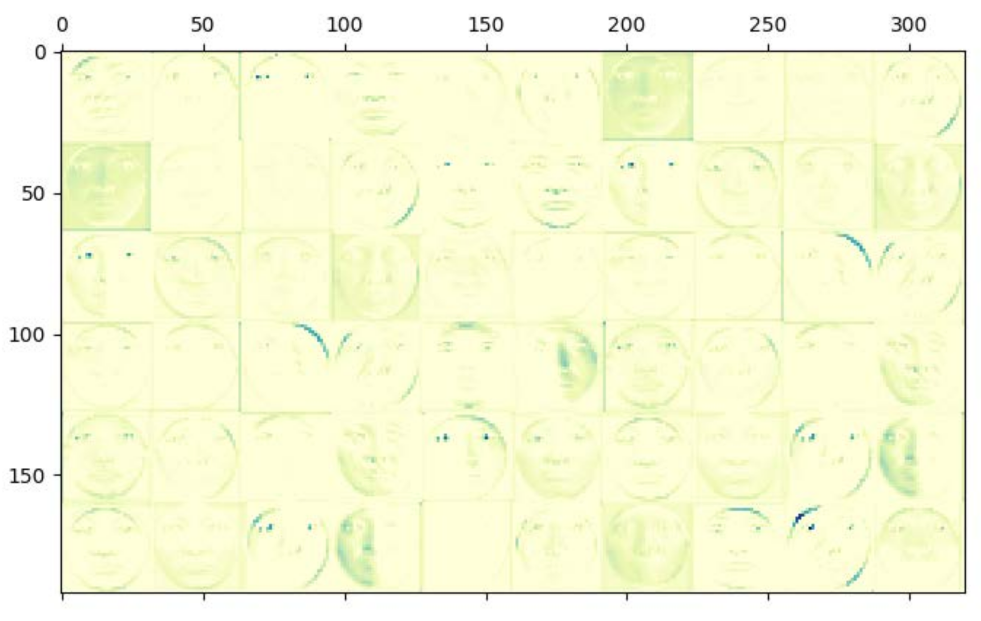
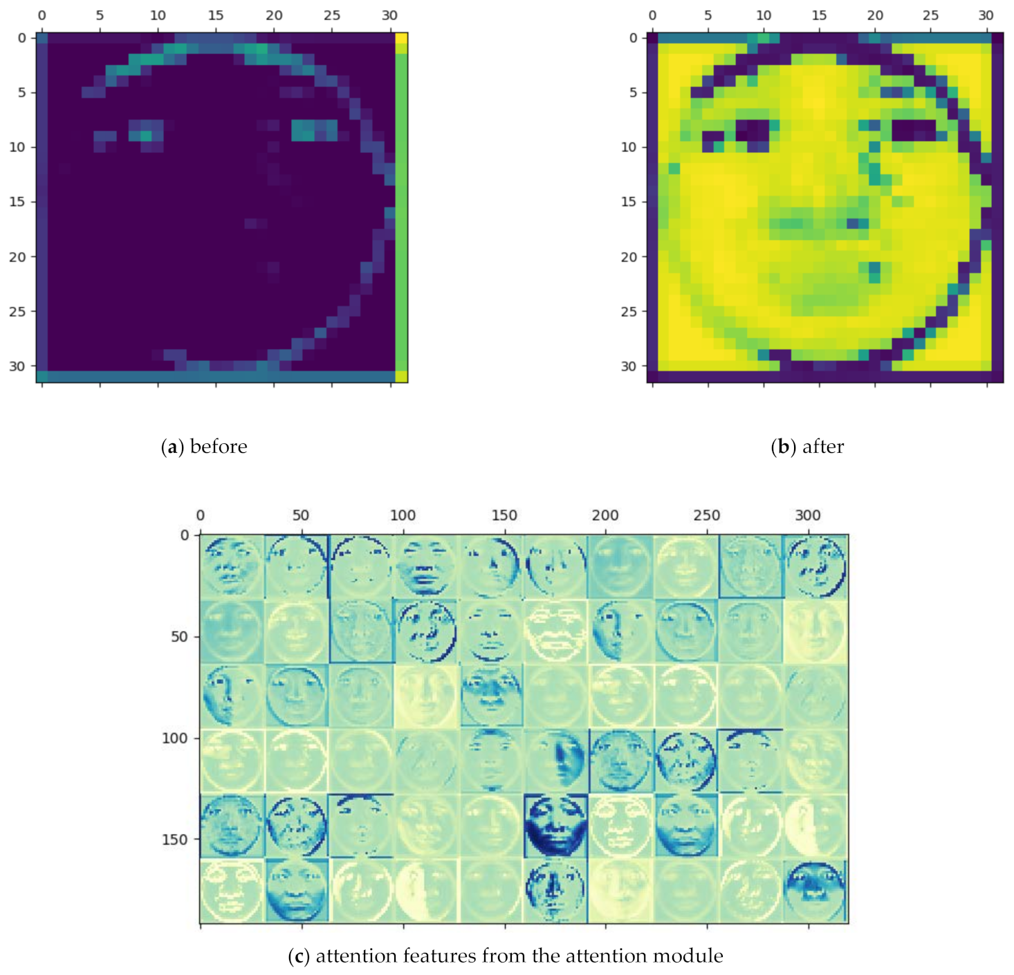
3.1. Performance of Attention Mechanism-Based Convolutional Feature Extractor

In order to evaluate the performance of the proposed attention-based convolutional feature extractor, the feature layers were extracted from the network for feature visualization. In this experiment, a randomly chosen face scan was used as the input for the network. The featured image of the face was output through the convolutional neural network, and Figure 7 shows the face feature visualization from the forth convolutional layer in the network, which was settled before the attention layer.

As shown in Figure 7, after the convolutional feature extraction network, 60 channels were selected for visualization in the output feature. It can be seen from the image that there were some features that could reflect the edge contour features of the face, such as the second in the first row. A feature map could reflect the size of the edge of the face; some could reflect the key parts of the face. For example, the seventh feature map in the first row clearly reflected the characteristics of the human nose, and the sixth in the third row feature map reflected the characteristics of a person’s mouth and chin. The extracted features were attended to by the subsequent attention layer. Figure 8 shows the feature change map after the attention superimposition.

It can be seen from Figure 8 that after superimposing the attention mechanism, most of the useful face areas became more obvious compared to those in Figure 7. This is because the attention mechanism used softmax as the activation function, so most areas gave a relatively low value, it had a feature suppression effect, which improved the effectiveness of the information transmitted in the network, and further reduced the noise part that was not conducive to face recognition. It retained the effective area for distinguishing the face and inhibited the part that was invalid for face classification.

3.2. Performance of the Sparse Siamese Neural Network Evaluated

In this section, a group of experiments are described that were carried out by combining different modules in order to evaluate the effectiveness of the attention module and the sparse representation on the network model with the training error and accuracy. Four network models were selected and are discussed: two neural networks contained the attention layer, and the other two did not; their loss functions were the traditional contrast loss function and the sparse loss function, respectively. The details of these four models are listed in Table 1. Here, the margin of the contrast loss function was set as $\mathrm{Margin}=2.0$, and the boundary hyperparameter of the sparse loss function was set as $m=2$.

In this study, a total of 199 people in the FRGC v2.0 Database were randomly selected to construct 370 pairs of samples, and each experiment used 70% data for training, 15% for validation in the training progress, and 15% for testing. The model which achieved the best accuracy on the validation dataset was used to obtain the test result of the model in the test set. The experiments were conducted five times to obtain the average accuracy and the results are presented in

Table 2. Accuracy of different network models on the testing set.

Models	Accuracy
Pure CNN with Contrastive Loss	81.00%
Attention CNN with Contrastive Loss	89.55%
Pure Siamese with Contrastive Loss	94.52%
Pure Siamese with Sparse Loss	94.85%
Attention Siamese with Contrastive Loss	95.24%
Attention Siamese with Sparse Loss	95.33%

.

In Table 2, the model with the attention module had a higher accuracy compared to the results of the first two models. The model with an attention module focused more on useful features and contained more trainable parameters, which improved generalization ability. The results proved the effectiveness of the attention module. Comparing the results of the first four network models, Siamese network structure achieved recognition accuracy of 94%, which had a significant improvement over the single branch network structure. The attention mechanism or the sparse loss function added into a Siamese network could also increase the accuracy, but the improvement was very small (less than 1%) compared to that of Siamese network structure.

3.3. Sample Size Comparison and Discussion

A large number of people with only few face scans from each person for training is common when building a face recognition system. However, a small sample size will restrict the training sample size of the traditional end to end deep learning method, which reduces the accuracy of the whole network. The Siamese network with two branch structure was adopted in this paper to resolve this problem, and we conducted experiments to compare with the traditional deep learning method. The ResNet50 was a typical STOA for classification tasks and was used as the example end-to-end model for comparison. In order to simulate the partial situation, we evaluated the recognition rate with a small size for training. A total of 190 people with five face scans for each person were used as the dataset. The training set face scan number from each person was controlled to be different among experiments and the rest of the face scans were used as the test set. These experiments were repeated five times to obtain the average accuracy in different situations.

The result is presented in

Table 3. Accuracy of face recognition under different sample situations.

Number of People in Training Set	End-to-End Model			Ours
	4	3	2	4	3	2
20	0.810	0.700	0.640	0.890	0.840	0.810
40	0.865	0.755	0.675	0.905	0.865	0.842
60	0.876	0.774	0.717	0.924	0.901	0.853
80	0.895	0.840	0.808	0.935	0.910	0.855
100	0.820	0.758	0.726	0.936	0.918	0.860
120	0.774	0.703	0.628	0.942	0.922	0.886
140	0.813	0.708	0.661	0.957	0.930	0.878
160	0.801	0.743	0.683	0.943	0.914	0.885
180	0.765	0.731	0.658	0.953	0.920	0.891

, and shows that the recognition accuracy of the traditional end-to-end method dropped with the increase in the number of people. The recognition rate was high when the sample number was small, and the end-to-end method reached the highest recognition rate on the face dataset with a training set size of 80. However, the end-to-end model dropped quickly and the recognition accuracy decreased to 0.765 when the number of people increased to 180. The accuracy of the end-to-end model decreased when the training set number decreased as well. In comparison, the proposed method showed a good performance to scale with a larger number of people and a smaller size of training set than the traditional end-to-end method. It proved that the proposed method can perform well in a small sized situation.

4. Conclusions

This study has developed a new face recognition algorithm based on 3D face scan data with the attention mechanism and sparse representation. The weight of the network is shared by constructing a Siamese network optimized with a sparse loss function. The established model can ensure not only better face recognition performance but also a smaller encoding size. The results showed that the proposed ACNN can extract features from the preprocessed 3D-scanned faces and eliminate the redundant areas at the same time. The attention mechanism gave the network an improvement in recognition accuracy of about 8% in the single branch network model. The sparse representation in the proposed method enabled it to be trained with minimal scan data to obtain a face coding for matching. The Siamese network structure had a significant improvement over the single branch network structure. The proposed method has potential to achieve high-accuracy face recognition.

However, although the sparse representation is utilized in this study to reduce the coding space, the redundant output neurons were not removed from the structure of the network which would cause extra computational cost and limit its use. In our future work, the combination of neural network pruning and sparse representation can be applied to improve the recognition efficiency and reduce complexity of the network, so that the proposed method could be applied in industries and in medical treatment by integrating the hardware such as Nvidia Jetson Nano.

References

1. Masi, I.; Wu, Y.; Hassner, T.; Natarajan, P. Deep Face Recognition: A Survey. In Proceedings of the 31st SIBGRAPI Conference on Graphics, Patterns and Images, SIBGRAPI 2018, Parana, Brazil, 29 Octorber–1 November 2018; pp. 471–478. [Google Scholar] [CrossRef]
2. Gsaxner, C.; Pepe, A.; Li, J.; Ibrahimpasic, U.; Wallner, J.; Schmalstieg, D.; Egger, J. Augmented Reality for Head and Neck Carcinoma Imaging: Description and Feasibility of an Instant Calibration, Markerless Approach. Comput. Methods Programs Biomed. 2020, 200, 105854. [Google Scholar] [CrossRef] [PubMed]
3. Wang, M.; Deng, W. Deep face recognition: A survey. Neurocomputing 2021, 429, 215–244. [Google Scholar] [CrossRef]
4. Adjabi, I.; Ouahabi, A.; Benzaoui, A.; Taleb-Ahmed, A. Past, present, and future of face recognition: A review. Electronics 2020, 9, 1188. [Google Scholar] [CrossRef]
5. Cootes, T.F.; Edwards, G.J.; Taylor, C.J. Active Appearance Models. IEEE Trans. Pattern Anal. Mach. Intell. 2001, 23, 681–685. [Google Scholar] [CrossRef] [Green Version]
6. Xiaofei, H.; Shuicheng, Y.; Yuxiao, H.; Partha, N.; Hong-Jiang, Z. Face Recognition Using Laplacianfaces. IEEE Trans. Pattern Anal. Mach. Intell. 2005, 27, 328–340. [Google Scholar] [CrossRef]
7. Ze, L.; Xudong, J.; Alex, K. A novel lbp-based color descriptor for face recognition. In Proceedings of the IEEE International Conference on Acoustics, Speech and Signal Processing 2017, New Orleans, LA, USA, 5–9 March 2017; pp. 1857–1861. [Google Scholar]
8. Déniz, O.; Bueno, G.; Salido, J.; De La Torre, F. Face recognition using Histograms of Oriented Gradients. Pattern Recognit. Lett. 2011, 32, 1598–1603. [Google Scholar] [CrossRef]
9. Li, W.J.; Wang, J.; Huang, Z.H.; Zhang, T.; Du, D.K. LBP-like feature based on Gabor wavelets for face recognition. Int. J. Wavelets Multiresolution Inf. Process. 2017, 15, 1750049. [Google Scholar] [CrossRef]
10. Leo, M.J.; Suchitra, S. SVM based expression-invariant 3D face recognition system. Procedia Comput. Sci. 2018, 143, 619–625. [Google Scholar] [CrossRef]
11. Sarma, M.S.; Srinivas, Y.; Abhiram, M.; Ullala, L.; Prasanthi, M.S.; Rao, J.R. Insider threat detection with face recognition and KNN user classification. In Proceedings of the 2017 IEEE International Conference on Cloud Computing in Emerging Markets CCEM 2017, Bangalore, India, 1–3 November 2017; pp. 39–44. [Google Scholar] [CrossRef]
12. Ding, C.; Tao, D. Trunk-Branch Ensemble Convolutional Neural Networks for Video-Based Face Recognition. IEEE Trans. Pattern Anal. Mach. Intell. 2018, 40, 1002–1014. [Google Scholar] [CrossRef] [Green Version]
13. Yang, J.; Adu, J.; Chen, H.; Zhang, J.; Tang, J. A Facial Expression Recongnition Method Based on Dlib, RI-LBP and ResNet. J. Phys. Conf. Ser. 2020, 1634. [Google Scholar] [CrossRef]
14. Almabdy, S.; Elrefaei, L. Deep convolutional neural network-based approaches for face recognition. Appl. Sci. 2019, 9, 4397. [Google Scholar] [CrossRef] [Green Version]
15. Xie, S.; Liu, S.; Chen, Z.; Tu, Z. Attentional ShapeContextNet for Point Cloud Recognition. In Proceedings of the 2018 IEEE/CVF Conference on Computer Vision and Pattern Recognition, Salt Lake City, UT, USA, 18–23 June 2018; pp. 4606–4615. [Google Scholar] [CrossRef]
16. Ghojogh, B.; Ghodsi, A.L.I.; Ca, U. Attention Mechanism, Transformers, BERT, and GPT: Tutorial and Survey. 2020. Available online: https://doi.org/10.31219/osf.io/m6gcn (accessed on 13 October 2021).
17. Li, W.; Liu, K.; Zhang, L.; Cheng, F. Object detection based on an adaptive attention mechanism. Sci. Rep. 2020, 10, 1–13. [Google Scholar] [CrossRef]
18. Li, J.; Jin, K.; Zhou, D.; Kubota, N.; Ju, Z. Attention mechanism-based CNN for facial expression recognition. Neurocomputing 2020, 411, 340–350. [Google Scholar] [CrossRef]
19. Liao, M.; Gu, X. Face recognition approach by subspace extended sparse representation and discriminative feature learning. Neurocomputing 2020, 373, 35–49. [Google Scholar] [CrossRef]
20. Liu, S.; Li, L.; Jin, M.; Hou, S.; Peng, Y. Optimized coefficient vector and sparse representation-based classification method for face recognition. IEEE Access 2020, 8, 8668–8674. [Google Scholar] [CrossRef]
21. Deng, X.; Da, F.; Shao, H.; Jiang, Y. A multi-scale three-dimensional face recognition approach with sparse representation-based classifier and fusion of local covariance descriptors. Comput. Electr. Eng. 2020, 85, 106700. [Google Scholar] [CrossRef]
22. Sun, Y.; Wang, Y.; Liu, Z.; Siegel, J.E.; Sarma, S.E. PointGrow: Autoregressively Learned Point Cloud Generation with Self-Attention. In Proceedings of the IEEE Winter Conference on Applications of Computer Vision (WACV), Snowmass Village, CO, USA, 1–5 March 2020; pp. 61–70. [Google Scholar] [CrossRef]
23. Soltanpour, S.; Boufama, B.; Jonathan Wu, Q.M. A survey of local feature methods for 3D face recognition. Pattern Recognit. 2017, 72, 391–406. [Google Scholar] [CrossRef]
24. Tang, H.; Yin, B.; Sun, Y.; Hu, Y. 3D face recognition using local binary patterns. Signal Process. 2013, 93, 2190–2198. [Google Scholar] [CrossRef]
25. Lei, Y.; Bennamoun, M.; Hayat, M.; Guo, Y. An efficient 3D face recognition approach using local geometrical signatures. Pattern Recognit. 2014, 47, 509–524. [Google Scholar] [CrossRef]
26. Liu, F.; Zhao, Q.; Liu, X.; Zeng, D. Joint Face Alignment and 3D Face Reconstruction with Application to Face Recognition. IEEE Trans. Pattern Anal. Mach. Intell. 2020, 42, 664–678. [Google Scholar] [CrossRef] [Green Version]
27. You, H.; Feng, Y.; Ji, R.; Gao, Y. PVNet: A Joint Convolutional Network of Point Cloud and Multi-View for 3D Shape Recognition. In Proceedings of the 26th ACM International Conference on Multimedia, Seoul, Korea, 22–26 October 2018; pp. 1310–1318. [Google Scholar]
28. Zhang, Z.Y.; Da, F.; Yu, Y. Data-Free Point Cloud Network for 3D Face Recognition. arXiv 2019, arXiv:1911.04731. [Google Scholar]
29. Ahmed, N.K.; Hemayed, E.E.; Fayek, M.B. Hybrid siamese network for unconstrained face verification and clustering under limited resources. Big Data Cogn. Comput. 2020, 4, 19. [Google Scholar] [CrossRef]
30. Phillips, P.J.; Flynn, P.J.; Scruggs, T.; Bowyer, K.W.; Chang, J.; Hoffman, K.; Marques, J.; Min, J.; Worek, W. Overview of the face recognition grand challenge. In Proceedings of the 2005 IEEE Computer Society Conference on Computer Vision and Pattern Recognition, CVPR 2005, San Diego, CA, USA, 20–25 June 2005; Volume 1, pp. 947–954. [Google Scholar] [CrossRef]
31. Mian, A.S.; Bennamoun, M.; Owens, R. An efficient multimodal 2D-3D hybrid approach to automatic face recognition. IEEE Trans. Pattern Anal. Mach. Intell. 2007, 29, 1927–1943. [Google Scholar] [CrossRef] [PubMed] [Green Version]
32. Koenderink, J.J.; van Doorn, A.J. Surface shape and curvature scales. Image Vis. Comput. 1992, 10, 557–564. [Google Scholar] [CrossRef]
33. Kang, I.G.; Park, F.C. Cubic spline algorithms for orientation interpolation. Int. J. Numer. Methods Eng. 2015, 46, 45–64. [Google Scholar] [CrossRef]
34. Huang, Z.; Zhu, T.; Li, Z.; Ni, C. Non-Destructive Testing of Moisture and Nitrogen Content in Pinus Massoniana Seed-ling Leaves with NIRS Based on MS-SC-CNN. Appl. Sci. 2021, 11, 2754. [Google Scholar] [CrossRef]
35. Wang, J.; Li, Z.; Chen, Q.; Ding, K.; Zhu, T.; Ni, C. Detection and Classification of Defective Hard Candies Based on Image Processing and Con-volutional Neural Networks. Electronics 2021, 10, 2017. [Google Scholar] [CrossRef]
36. Woo, S.; Park, J.; Lee, J.Y.; Kweon, I.S. CBAM: Convolutional Block Attention Module. In Proceedings of the European Conference on Computer Vision in Lecture Notes in Computer Science, Munich, Germany, 8–14 September 2018; Springer International Publishing: Cham, Switzerland, 2018; Volume 11211, pp. 3–19. [Google Scholar] [CrossRef] [Green Version]
Figure 1. The preprocessing progress and example result generated by the 3D face data conversion. (a) The preprocessing schemes of the obtained 3D point cloud data. The small red sphere marked the nose tip point, and the blue sphere retained the nose tip point as the center with a radius of 90 mm. The gray surface is the curved face area. (b) The example 2D face grayscale images.
Electronics 10 02539 g001
Figure 2. Structural chart of face recognition with attention mechanism and sparse representation.
Electronics 10 02539 g002
Figure 3. Structure of the attention module coupled with the convolutional module.
Electronics 10 02539 g003
Figure 4. Structure of attention mechanism and sparse loss Siamese neural network.
Electronics 10 02539 g004
Figure 5. Characteristics of the loss function.
Electronics 10 02539 g005
Figure 6. Loss function output space map.
Electronics 10 02539 g006
Figure 7. Face feature visualization from the forth convolutional layer.
Electronics 10 02539 g007
Figure 8. Face feature visualization before and after the attention module.
Electronics 10 02539 g008