Article

Parametric Analysis of Linear Periodic Arrays Generating Flat-Top Beams

1
RF Payloads and Technology Division, European Space Agency, 2200 Noordwijk, The Netherlands
2
Department of Engineering and Architecture, University of Trieste, Via A. Valerio 10, 34127 Trieste, Italy
*
Author to whom correspondence should be addressed.
Electronics 2021, 10(20), 2452; https://doi.org/10.3390/electronics10202452
Submission received: 1 July 2021 / Revised: 30 September 2021 / Accepted: 5 October 2021 / Published: 9 October 2021
(This article belongs to the Special Issue High-Performance Antenna Design and Applications)

Abstract

:
Several synthesis techniques are available to optimize amplitude and phase excitations of periodic linear arrays to generate flat-top beams. Clearly, the optimal tapering depends on design parameters such as the array length, the number of array elements, the beam flatness, the beam width, the side lobe levels, and others. In this paper, in order to derive useful guidelines and rule of thumb for the synthesis of periodic array antennas, relations between these parameters are derived employing linear programming techniques, which guarantee optimality of the solutions. Such relations are then plotted and used in some design examples.

1. Introduction

In this paper, the canonical problem of generating a flat-top beam with a linear array of equally spaced identical elements is investigated. A flat-top beam is a radiation pattern having an intensity profile that is flat over a required region of interest. Several antenna applications, such as reconnaissance and search RADARs, and wide-area broadcasting communication systems, require flat-top beams characterized by well-defined beamwidths. For such applications, key radiation pattern requirements are the ripple within the main-beam and the level of sidelobes after a transition zone from the main beam. Well-established synthesis procedures such as Fourier [1] or Woodward–Lawson [2,3] exist but are not particularly well suited due to the Gibbs phenomenon. Inspired by Butterworth filters [4], Ksienski introduced an analytical procedure [5] (extended in [6]) which maximizes the smoothness of the radiation patter at the expenses of an enlarged transition zone. Notwithstanding their speed, these techniques result suboptimal due to the unnecessary constraint on the realness of the voltage radiation pattern. In this respect, linear programming techniques allow for finding the global optimal solution to the flat-top power pattern problem [7].
Given an array geometry (i.e., the elements positions), the problem of the optimization of array excitations to satisfy arbitrary upper and lower bounds for the main beam and sidelobes is casted in the equivalent problem of the optimization of the real and imaginary parts of the autocorrelation of the excitations, which become the new unknowns. In this auxiliary space, the power pattern is a linear transformation of the unknowns (as the voltage pattern is a linear function of the array excitations) and the power pattern constraints can be described as linear constraints on the unknowns (an additional linear constraint on the positivity of the power pattern must be added). The goodness of this transposition stays in the fact that the minimization of the sidelobes and/or of the main-beam ripple become convex problems admitting a unique global solution, which can be found with linear programming techniques. Although the formulation [7] used in the following sections leverages on the framework developed by L. R. Rabiner in 1972 for Finite-Impulse-Response (FIR) filters [8,9], the application to array antennas and optimality aspects can be found in [10].
Concerning the computational speed of linear programming solvers, while the theoretical analyses of their complexity remain an open problem, the simplex method or the interior point methods have been shown to exhibit typical polynomial (in the number of unknowns and constraints) running times (which correspond to few seconds in the instances of the addressed problem) [11]. Notwithstanding the global optimality of the linear programming solution for a specified flat-top-beam problem, the sensitivity of the solution to the input parameters has not been addressed in the technical literature (to the best knowledge of the authors). This paper analyzes the performance relationships between the following design parameters: array length, number of array elements, beam width, maximum allowed beam ripple, and width of the transition region between the main beam and the side lobes. Adopting a linear programming approach, the optimal value of the maximum side lobe level is derived and graphically illustrated as a function of the other parameters. The study presented in this paper does not aim to propose a new array synthesis algorithm but rather to deepen the analyses presented in [7] to provide antenna engineers with some design curves giving useful insights in the problem and data for the preliminary phase of synthesis.
In addition to the analytical methods [1,2,3,4,5,6], the literature offers a great variety of numerical methods for the array synthesis. As an example, in [12,13,14], deterministic procedures are proposed based on alternating projection approaches; in [15], a linear programming optimization plus a polynomial factorization is conceived; and [16] proposes a fast and versatile deterministic algorithm that iteratively minimizes a suitable weighted cost function. Furthermore, many global optimization techniques have been proposed, such as those presented in [17,18], based on genetic algorithms; the one proposed in [19], based on the differential evolution algorithm; and that in [20], which exploits the particle swarm optimization approach. Although this canonical problem has been already investigated, to the knowledge of the authors, attention has never been focused on the relations between the abovementioned design parameters. The authors believe that such an analysis may be very useful in the preliminary phase of design. For example, using the curves shown in Section 3, the antenna designer can estimate the length of the linear array necessary to achieve certain assigned performances or can anticipate the expected pattern characteristics of a flat-top beam realizable with an array having a given length.
The paper is organized as follows. In Section 2 the problem is formulated. In Section 3 the dependence of the maximum side lobe level on various design parameters is presented and discussed along with an asymptotical analysis aimed to verify the results with respect to the number of pattern samples utilized to derive the relations between the design parameters. In Section 4 some numerical examples are presented in order to describe how the reference curves can be used and to prove the superiority of the linear programming compared with conventional methods for the synthesis of shaped beams. The conclusions are proposed in Section 5.

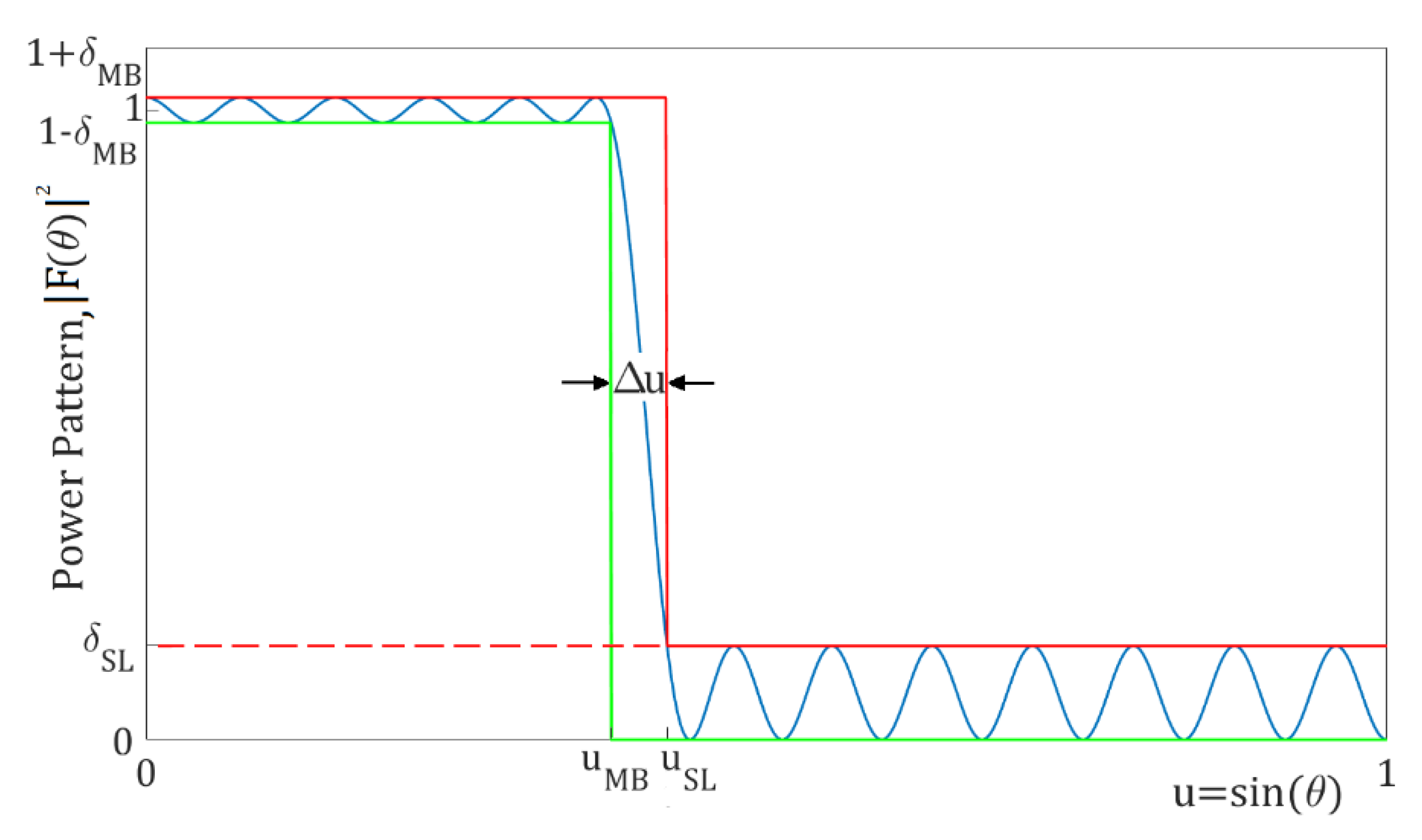
2. Formulation of the Problem

The array factor of a linear antenna array of N identical equally spaced elements is given by the following:
F ( ϑ ) = n = 0 N 1 E n e j k 0 n d u
where E n is the excitation of the n-th element; j = 1 ;   k 0 = 2 π / λ , with λ the wavelength; d is the inter-element spacing; and u = sin θ , where θ is the angle from broadside. In the sequel, the power pattern | F ( ϑ ) | 2 will be considered.
A flat-top beam pattern can be characterized by the main beam edge u M B , the ripple δ M B in the main beam, the maximum side lobe level δ S L , and the side lobe edge u S L , as depicted in Figure 1. The additional parameters Δ u = u S L u M B and K = δ M B / δ S L are also introduced.
The aim of the investigation presented in this paper is to derivie the relations between the above design parameters, exploiting them in the synthesis of flat-top beams. With this in mind, the desired values of u M B , u S L (or, alternatively, Δ u ), and δ M B (or, alternatively, K ) are imposed, and the power pattern is calculated in such a way as to satisfy the constraints imposed on these parameters, simultaneously minimizing the maximum side lobe level δ S L . This problem is solved by using a linear programming approach, as briefly explained below (see [8,9] for further details). At first, the power pattern is written as follows:
| F ( ϑ ) | 2 = n = ( N 1 ) N 1 R n e j k 0 n d u
where
R n = { i = n N 1 E i E i n *     i f   0 n ( N 1 ) i = n N 1 E i * E i + n   i f ( N 1 ) n < 0
with the asterisk denoting complex conjugate. By (3), R n = R n * . Therefore, (2) can be written in the following form:
| F ( ϑ ) | 2 = A 0 + 2 n = 1 N 1 ( A n cos ( k 0 n d u ) B n sin ( k 0 n d u ) ) ,
with R n = A n + j B n and in particular R 0 = i = 0 N 1 | E i | 2 = A 0 . The design parameters u M B ,   u S L ,   δ M B , and δ S L are then used to define a mask for the power pattern in (2). Such a mask is illustrated in Figure 1. Thanks to the auxiliary variables R n in (2) and (3), the power pattern synthesis is formulated as a linear programming problem, where the objective function to be minimized is δ S L . The problem can be formulated as follows:
minimize { δ S L }
subject to the following constraints:
| F ( u ) | 2 L ( u )
| F ( u ) | 2 U ( u )
δ S L 0
δ M B = δ M B d e s   o r   δ S L = δ M B / K d e s
where L ( u ) and U ( u ) are two positive functions representing, respectively, the lower and the upper bound of the mask, and are defined as
L ( u ) = ( 1 δ M B ) L E ( u , u M B )
U ( u ) = ( 1 + δ M B δ S L ) L T ( u , u S L ) + δ S L
Note that the constraints in (5) impose that the power pattern belong to the mask specified by L ( u ) and U ( u ) (conditions (5a) and (5b)), in which δ S L 0 (condition (5c)), and impose a desired value to δ M B or, alternatively, to K (condition (5d)). The solution of the linear programming problem in (5) provides the values of the variables R n of an equi-ripple power pattern, which perfectly fits between the lower and upper masks and exhibits the minimum attainable δ S L .
In the next section, several curves representing the relations between the design parameters are illustrated. Such results are obtained by sampling the synthesized radiation patterns on a set of equally spaced points in the visibility interval [ 1 ; 1 ] . Subsequently, the asymptotic behavior of the results is numerically analyzed by adopting an increasing number of samples. Three examples of array synthesis are presented in Section 4, and are solved with the aid of the obtained curves involving the design parameters.

3. Maximum Sidelobe Level vs. Design Parameters

In the sequel, a linear array with inter-element spacing d = λ / 2 will be considered, and the dependence of the maximum side lobe level on the other design parameters is derived and plotted for some test cases, by using the above described linear programming approach.

3.1. Case of Equality between Main Beam Width and Side Lobe Region Width

First, let us analyze the case where the main beam width ( u M B ) is equal to the side lobe region width ( 1 u S L ), that is u M B + u S L = 1 , and in (5d) K d e s = δ M B / δ S L = 1 (i.e., δ M B = δ S L = δ ). Figure 2 shows δ as a function of the transition width Δ u . In the figure, different curves refer to different values of N . As expected, higher values of Δ u correspond to lower values of δ as well as higher values of N correspond to lower values of δ . Thus, lower side lobes can be obtained with larger arrays or by allowing for a larger transition region.
From now on, unlike the previous case, flat-top beams are considered with u M B and 1 u S L possibly different, and δ M B possibly different from δ S L (i.e., K d e s 1 ).

3.2. Dependence on N

Figure 3a,b show the maximum side lobe level δ S L as a function of N . Both figures refer to the case u M B = 0.375 . As expected, the more stringent the constraints (that is, the values of Δ u and δ M B are lower), the higher the obtained values of maximum side lobe levels. The curves in Figure 3a are obtained with δ M B = 0.1 and Δ u = 0.05 ,   0.1 ,   0.15 , whereas those in Figure 3b refer to the case Δ u = 0.1 and δ M B = 0.02 ,   0.1 ,   0.2 . In both figures, the curves show a quasi-linear behavior. However, the curves in Figure 3b exhibit nearly the same slope, unlike those in Figure 3a.

3.3. Dependence on K

The dependence of the maximum side lobe level δ S L on K ( = δ M B / δ S L ) is analyzed here. In the next three figures, the same main beam edge u M B = 0.5 is considered, and the maximum side lobe level decreases as K increases. In Figure 4a, which corresponds to Δ u = 0.2 , all curves are practically linear. Instead, in Figure 4b, corresponding to Δ u = 0.15 , for high values of K , the curve obtained for N = 20 is nonlinear. In Figure 4c, corresponding to Δ u = 0.1 , the behavior is quasi-linear only for N = 40 .

3.4. Dependence on δ M B

Figure 5 shows the maximum side lobe level as a function of δ M B , through the parameter τ M B = ( 1 + δ M B ) / ( 1 δ M B ) expressed in dB (the parameter τ M B is used in agreement with several other papers, for example [9]). As expected, the maximum side lobe level is lower for higher values of δ M B : in other words, when relaxing the requirements for the maximum allowed ripple amplitude in the main beam, a reduction in the maximum side lobe level is observed. Moreover, the different curves refer to different values of Δ u . All curves have nearly the same shape and show that larger transition regions permit achieving better side lobe levels. All curves refer to the case u M B = 0.46 and N = 20 .

3.5. Dependence on u M B

Figure 6a shows the maximum side lobe level δ S L as a function of u M B for a maximum allowed beam ripple δ M B = 0.05 and a transition region Δ u varying from 0.05 to 0.2 . As expected, larger transition regions globally allow for lower maximum side lobe levels, but δ S L does not vary monotonically as a function of u M B : all curves show the same behavior, with alternating maxima and minima. However, the average slope of the curves and the differences between maxima and minima tend to increase when increasing of Δ u .
Figure 6b shows the maximum side lobe level as a function of the main beam edge u M B for an assigned beam ripple δ M B = 0.05 . All of the curves in the figure refer to a transition region Δ u = 0.15 and to different values of N , varying from N = 18 to N = 22 . It is interesting to note that all curves show a similar behavior. As expected, lower side lobe levels can be obtained with higher values of N . However, for certain values of u M B , corresponding to the minima along the curve obtained with N elements, the corresponding values of δ S L are nearly coincident with the values obtained with N + 1 elements. Moreover, for low values of u M B , the maximum of the curve corresponding to N elements is higher compared with the closest minimum of the curve with N + 1 elements.

3.6. Dependence on δ M B

Figure 7 shows the maximum side lobe level as a function of the transition region Δ u for u M B = 0.16 and different values of δ M B from 0.01 to 0.5 . All curves are decreasing, but their behavior is not linear. Observe that the light blue curve, corresponding to δ M B = 0.05 , contains the same values obtainable when sampling the curves in Figure 6a for u M B = 0.16 .

3.7. Asymptotical Analysis

The above numerical results have been obtained by sampling the power patterns on a grid of N s = 800 equally spaced points in the interval [ 1 ; 1 ] . In order to verify the asymptotic stability of the results, we applied the adopted method of synthesis and re-calculated the above curves using different numbers N s of samples. For example, with reference to the already discussed Figure 7, which corresponds to N = 20 and u M B = 0.16 , we set δ M B = 0.1 and analyzed the dependence of δ S L on Δ u for N s going from 200 to 3200 . Figure 8 shows the results obtained.
Different curves correspond to different values of N s . As it can be seen, the results nearly independent of the number of samples. In order to better illustrate the convergence, Figure 9 shows the maximum side lobe level as a function of the number of samples for N = 20 ,   u M B = 0.16 , and Δ u = 0.7 . Note that the curve tends to saturate rapidly when increasing the number of samples. Thus, the results prove the effectiveness of the adopted method to calculate the relations between the design parameters, showing a behavior quasi-independent of the number of points on which the power patterns have been sampled.

4. Examples

In this section, three significant examples are proposed, which show how the above derived curves can help in the preliminary design phase of linear antenna arrays radiating flat-top beams.

4.1. First Example: Case of Equality between Main Beam Width and Side Lobe Region Width

Let us assume that a linear array composed by N = 30 elements is required to radiate a flat-top beam, with the main beam region and the side lobe region having the same width (i.e., u M B + u S L = 1 ), and K = 1 (i.e, δ M B = δ S L = δ ). We want to find the maximum beam width (or, equivalently, the minimum transition region Δ u ), which guarantees a maximum side lobe level δ S L 15 dB. Using the curve corresponding to N = 30 in Figure 2, we can observe that a value Δ u = 0.055 can give a power pattern satisfying the required specifications. In fact, using the linear programming with u M B = 0.5 Δ u 2 = 0.4725 , u S L = 0.5 + Δ u 2 = 0.5275 , and K = 1 , we obtain the radiation pattern of Figure 10a, with a maximum side lobe level of 15.68 dB and a maximum allowed ripple in the main beam (shown in the inset of Figure 10a) of δ = 0.027 , which corresponds to τ M B = 10 log 10 ( ( 1 + δ ) / ( 1 δ ) ) = 0.23 . The CPU time for this example is approximately 0.1 s.

4.2. Second Example: Estimation of the Number of Elements

As a second example, we want to produce a flat-top beam with the following values for the design parameters: u M B = 0.375 , Δ u = 0.1 , δ M B = 0.02 , and δ S L 30 dB. With the help of Figure 3b, we note that an array of N = 27 elements can achieve the required performances. In fact, using the linear programming with these parameters yields the power pattern of Figure 10b, which satisfies the constraints. The CPU time for this example is slightly lower than 0.1 s.

4.3. Third Example: Estimation of the Width of the Transition Region

Let us consider a linear antenna array composed by N = 20 elements. We want to radiate a flat-top beam with a beamwidth u M B = 0.46 , a maximum side lobe level of 30 dB and a maximum allowed ripple in the main beam region δ M B = 0.0575 ( τ M B = 0.5 dB). The curves in Figure 5 suggest that a possible value of width of the transition region that allows us to satisfy the requirement is Δ u = 0.125 . In fact, using the linear programming with these parameters yields the power pattern in Figure 10c, which satisfies all of the constraints. The CPU time for this example is slightly lower than 0.1 s.

4.4. Result Comparison

This final subsection aims to prove the superiority of the adopted linear programming in terms of constraint compliance for the flat-top beam synthesis. Precisely, the previous three examples have been solved with two well-known methods, i.e., the Fourier Transform approach [1] and the Woodward–Lawson technique [2]. Figure 11 shows the patterns obtained by the three methods. As it can be seen, only the linear programming always satisfies the imposed constraints, whereas the classical methods may fail to meet the requirements. On the other hand, both the Woodward–Lawson technique and the Fourier Transform approach have the advantage of using closed-form expressions for the addressed problems. Thus, the CPU times are quite low (approximately 1 ms or even less).

5. Conclusions

The power synthesis of flat-top beams for linear periodic arrays is a well-known canonical problem in the antenna community. The shape of the synthesized pattern depends on a number of design parameters, such as the array length, the beam width, the maximum allowed ripple in the main beam region, the width of the transition region, and the maximum side lobe level.
The aim of this paper was to derive the relations between these design parameters and to use them for design purposes. Adopting a linear programming technique that guarantees the optimality of the solutions, several case studies were analyzed, obtaining a set of relations between the above parameters, which are represented graphically by curves that can be useful in the array design. Three examples of array design were proposed, and solved with the aid of these curves, obtaining results fully compliant with the assigned masks. In particular, the curves show that, also for the simple case of linear equally spaced arrays, the relations between the design parameters can be nonlinear. This is an interesting and not completely expected result, which must be taken into account in the array design.

Author Contributions

P.A. and G.B.: conceptualization, review and editing, G.B.: conceptualization, software, and original draft preparation, G.T.: conceptualization, writing and validation, R.V.: conceptualization. All authors have read and agreed to the published version of the manuscript.

Funding

This research received no external funding.

Conflicts of Interest

The authors declare no conflict of interest.

References

  1. Dunbar, A.S. On the Theory of Antenna Beam Shaping. J. Appl. Phys. 1952, 23, 847–853. [Google Scholar] [CrossRef]
  2. Woodward, P.M. A Method for Calculating the Field Over a Plane Aperture Required to Produce a Given Polar Diagram. J. Inst. Electr. Eng. Part IIIA Radiolocat. 1946, 93, 1554–1558. [Google Scholar] [CrossRef]
  3. Woodward, P.M.; Lawson, J.D. The theoretical precision with which an arbitrary radiation pattern may be obtained from a source of a finite size. J. Inst. Electr. Eng. Part III Radio Commun. Eng. 1948, 95, 363–370. [Google Scholar]
  4. Butterworth, S. On the theory of filter amplifiers. Exp. Wirel. 1930, 7, 536–541. [Google Scholar]
  5. Ksienski, A. Maximally flat and quasi-smooth sector beams. IRE Trans. Antennas Propag. 1960, 8, 476–484. [Google Scholar] [CrossRef]
  6. Petrolati, D.; Angeletti, P.; Toso, G. Linear arrays with Maximally Flat Beams. In Proceedings of the Fourth European Conference on Antennas and Propagation, Barcelona, Spain, 12–16 April 2010. [Google Scholar]
  7. Angeletti, P.; Buttazzoni, G.; Toso, G.; Vescovo, R. Parametric analysis of flat top beam patterns generated by linear periodic arrays. In Proceedings of the 2016 10th European Conference on Antennas and Propagation (EuCAP), Davos, Switzerland, 10–15 April 2016; pp. 1–2. [Google Scholar]
  8. Rabiner, L.R. Linear program design of finite impulse response (FIR) digital filters. IEEE Trans. Audio Electroacoust. 1972, 20, 280–288. [Google Scholar] [CrossRef]
  9. Rabiner, L.R. The design of finite impulse response digital filters using linear programming techniques. Bell Syst. Tech. J. 1972, 51, 1177–1198. [Google Scholar] [CrossRef]
  10. Isernia, T.; Bucci, O.M.; Fiorentino, N. Shaped beam antenna synthesis problems: Feasibility criteria and new strategies. J. Electromagn. Waves Appl. 1998, 12, 103–138. [Google Scholar] [CrossRef]
  11. Karmarkar, N. A new polynomial-time algorithm for linear programming. Combinatorica 1984, 4, 373–395. [Google Scholar] [CrossRef]
  12. Bucci, O.M.; D’Elia, G.; Mazzarella, G.; Panariello, G. Antenna pattern synthesis: A new general approach. Proc. IEEE 1994, 82, 358–371. [Google Scholar] [CrossRef]
  13. Quijano, J.L.A.; Vecchi, G. Alternating adaptive projections in antenna synthesis. IEEE Trans. Antennas Propag. 2010, 58, 727–737. [Google Scholar] [CrossRef]
  14. Buttazzoni, G.; Vescovo, R. An efficient and versatile technique for the synthesis of 3D copolar and crosspolar patterns of phase-only reconfigurable conformal arrays with DRR and near-field control. IEEE Trans. Antennas Propag. 2014, 62, 1640–1651. [Google Scholar] [CrossRef]
  15. Isernia, T.; Morabito, A.F. Mask-constrained power synthesis of linear arrays with even excitations. IEEE Trans. Antennas Propag. 2016, 64, 3212–3217. [Google Scholar] [CrossRef]
  16. Comisso, M.; Buttazzoni, G.; Vescovo, R. Reconfigurable antenna arrays with multiple requirements: A versatile 3D approach. Int. J. Antennas Propag. 2017, 2017, 6752108. [Google Scholar] [CrossRef]
  17. Johnson, J.M.; Rahmat-Samii, Y. Genetic algorithms in engineering electromagnetics. IEEE Antennas Propag. Mag. 1997, 39, 7–21. [Google Scholar] [CrossRef] [Green Version]
  18. Haupt, R.L. Antenna design with a mixed integer genetic algorithm. IEEE Trans. Antennas Propag. 2007, 55, 577–582. [Google Scholar] [CrossRef]
  19. Yang, S.; Gan, Y.B.; Khiang, T.P. A new technique for power-pattern synthesis in time-modulated linear arrays. IEEE Antennas Wirel. Propag. Lett. 2003, 2, 285–287. [Google Scholar] [CrossRef]
  20. Zhou, R.; Sun, J.; Wei, S.; Wang, J. Synthesis of conformal array antenna for hypersonic platform SAR using modified particle swarm optimization. IET Radar Sonar Navig. 2017, 11, 1235–1242. [Google Scholar] [CrossRef]
Figure 1. Example of a constraints compliant radiation pattern and definition of the design parameters u M B , u S L , δ M B , δ S L , and Δ u for the flat-top power pattern.
Electronics 10 02452 g001
Figure 2. Case of equality between the main beam width and the side lobe region width, and K d e s = δ M B / δ S L = 1 : the curves show δ = ( δ M B = δ S L ) as a function of Δ u for N taking values from 20 to 30 .
Electronics 10 02452 g002
Figure 3. Maximum side lobe level δ S L (in dB) as a function of N , obtained with u M B = 0.375 and: (a) a common value of δ M B = 0.1 and varying Δ u ; (b) a common value of Δ u = 0.1 and varying δ M B .
Electronics 10 02452 g003
Figure 4. Maximum side lobe level δ S L (in dB) as a function of K . The curves are obtained for u M B = 0.5 and (a) Δ u = 0.2 , (b) Δ u = 0.15 , and (c) Δ u = 0.1 .
Electronics 10 02452 g004
Figure 5. Case Maximum side lobe level δ S L (in dB) as a function of the parameter τ M B = ( 1 + δ M B ) / ( 1 δ M B ) expressed in dB, where δ M B is the maximum allowed ripple amplitude, in the case where N = 20 and u M B = 0.46 , with different values of Δ u ranging from 0.05 to 0.2 .
Electronics 10 02452 g005
Figure 6. Maximum side lobe level δ S L (in dB) as a function of u M B , obtained for δ M B = 0.05 and (a) N = 20 with Δ u = 0.05 ,   0.125 ,   0.2 , (b) Δ u = 0.15 with N from 18 to 22 .
Electronics 10 02452 g006
Figure 7. Maximum side lobe level δ S L (in dB) as a function of Δ u , for N = 20 , u M B = 0.16 and δ M B varying from 0.5 to 0.01 .
Electronics 10 02452 g007
Figure 8. Maximum side lobe level δ S L (in dB) as a function of Δ u , for N = 20 , u M B = 0.16 , and the number of sampling points varying from 200 to 3200 .
Electronics 10 02452 g008
Figure 9. Maximum side lobe level (in dB) as a function of the number of samples, for N = 20 , u M B = 0.16 , and Δ u = 0.7 .
Electronics 10 02452 g009
Figure 10. The radiation patterns synthesized with the linear programming for the examples in (a) Section 4.1, (b) Section 4.2, and (c) Section 4.3. All of the patterns satisfy the imposed constraints.
Electronics 10 02452 g010aElectronics 10 02452 g010b
Figure 11. Comparison. The radiation patterns synthesized with the linear programming (blue lines), compared with the patterns of the Woodward–Lawson method (ciano lines) and those of the Fourier Transform approach (black lines) for the examples in (a) Section 4.1, (b) Section 4.2, and (c) Section 4.3. All of the patterns satisfy the imposed constraints.
Electronics 10 02452 g011
Publisher’s Note: MDPI stays neutral with regard to jurisdictional claims in published maps and institutional affiliations.

