Article

Study on the Lyapunov Stability of a Time-Discrete Macro Traffic System with Variable Delay and Feedback Control

1
College of Computer and Information Science, Southwest University, Chongqing 400715, China
2
College of Artificial Intelligence, Southwest University, Chongqing 400715, China
3
Instrumentation Technology and Economy Institute (ITEI), Beijing 100055, China
*
Author to whom correspondence should be addressed.
Electronics 2021, 10(19), 2346; https://doi.org/10.3390/electronics10192346
Submission received: 26 August 2021 / Revised: 20 September 2021 / Accepted: 22 September 2021 / Published: 25 September 2021
(This article belongs to the Section Industrial Electronics)

Abstract

:
This paper constructs and analyzes a time-discrete macro traffic system with bounded variable delay and feedback control strategy. By theoretical analysis using the Lyapunov theorem, a stable condition of the macro traffic system is derived under which traffic jams can be suppressed. The traffic developing properties of the new traffic system for different variable delay and feedback control parameters are illustrated through simulation. The results show that variable delay can easily lead a traffic system to evolve into a traffic jam, and the feedback control strategy can enhance the stability of the traffic system with respect to variable delay. Moreover, the traffic unstable level caused by variable delay is less than the unstable extent caused by the constant upper bound of variable delay; still it is more serious than the traffic fluctuation caused by the constant lower bound of variable delay.

1. Introduction

In the wake of a rapid increase in the number of automobiles, road traffic jams have become increasingly severe and have caused many troubles in our daily lives. The operating rules of the road traffic system and the reason for traffic jams should first be explored to reduce road traffic jams. We can then establish a more scientific traffic plan and improve the collaboration of traffic systems by using information technologies such as traffic communication, traffic computation and traffic control.
Many traffic models have been proposed from the micro or macro perspective to disclose the law of traffic jams. Generally, micro models chiefly focus on the kinetic behavior of a single vehicle, and macro models primarily study whole-road traffic properties. In terms of micro models, a famous model is the optimal velocity (OV) car-following model [1]. The OV model can describe a real stop-and-go traffic jam with a differential dynamic function. It was extensively researched to uncover special traffic properties in many different road situations. Jiao et al. [2] analyzed the safety and dynamic property of car-following behavior with collision sensitivity. Lee et al. [3] studied car-following behavior for a road with multiple lanes by integrating a deep learning method. Tordeux et al. [4] compared the traffic properties of car-following models with or without delayed information and explored the effect of reaction times on traffic stability. Treiber et al. [5] compared the performance metrics of four numerical integration schemes for car-following models. Chen et al. [6] investigated the influence of long-term and short-term driving characteristics on car-following behavior. Treiber et al. [7] studied reaction times, estimation errors and anticipation effect in micro traffic models. From the perspective of macro traffic modeling, Payne [8] proposed the famous density gradient model based on the car-following idea in 1971. After that, Aw et al. [9] established the early velocity gradient model. In 1998, by latticing the space variable in macro traffic modeling, Nagatani constructed the first lattice hydrodynamic model [10]. After the original density gradient model, the velocity gradient model and the lattice hydrodynamic model were proposed, many extended works have been carried out using these models. Some typical extended works, such as the model proposed by Khan et al. [11], considered transition velocities, the extended speed gradient model with different kinds of vehicles [12], the lattice hydrodynamic model with a consideration of traffic interruption [13], etc. In addition, there are many other famous traffic models such as intelligent driver models [14,15,16], cellular automaton models [17,18,19], cell transmission models [20,21,22], etc. They are also extensively used to describe many kinds of real traffic phenomena.
A traffic system operates cooperatively with many kinds of traffic information, particularly information acquired by vehicle-to-vehicle communication technology. When traffic information is changed, it is transformed and obtained by a target vehicle to adjust its motion. In this process, the motion state of the target vehicle cannot respond to the changed traffic information in a timely fashion, and delay is unavoidable. To uncover the impact of delay on traffic flow, Yu et al. [23] studied the impact of headway and velocity on car-following traffic. Li et al. [24] researched the impact of driver variables on delay using the car-following rule. Kang et al. [25] investigated the influence of drivers’ physical delay with respect to relative flux on traffic stability. Zhang [26] studied the influence of variable delay in sensing traffic density on traffic flow. This research shows that delay can lower traffic stability and cause traffic jams.
In the above research, the traffic models are continuous with respect to time. To investigate road traffic from the view of a time-discrete system, some research has been conducted using micro traffic modeling. In 2009, McCartney [27] investigated a time-discrete car-following model, constructed based on a logistic map. Recently, Zhu et al. [28] introduced a time-discrete car-following model by writing the continuous equation into a difference equation. In addition, cellular automaton models [17,18,19] can be categorized as a kind of time-discrete traffic model. The traffic flow properties of cellular automaton models are simulated by the four rules of acceleration, deceleration, randomization and vehicle motion. Cellular automaton models are very convenient for simulation, but they cannot be analyzed mathematically.
Through the above literature analysis, it is clear that delay is inevitable in real traffic conditions, and research on traffic modeling and analysis from the time-discrete system is scarce. To explicitly reveal the variable delay on traffic flow from the perspective of the time-discrete system by macro traffic modeling and reducing the adverse impact of delay on traffic stability, a time-discrete lattice hydrodynamic traffic model with variable delay and a feedback control method is proposed and studied in the following sections.
The remainder of this paper is arranged as follows: Section 2 introduces a new time-discrete traffic system; Section 3 explores the stability property of the new model. Section 4 covers simulation and analysis; Section 5 summarizes the conclusion.

2. The Time-Discrete Traffic System

The hydrodynamic model constructed by Nagatani [10] can be described as below:
t ρ ( x , t ) + x ( ρ v ( x , t ) ) = 0 t ( ρ v ( x , t ) ) = a ρ 0 V ( ρ ( x + σ , t ) ) a ( ρ v ( x , t ) ) ,
where ρ ( x , t ) and ρ v ( x , t ) , respectively, indicate the local density and local traffic flux of position x at time t , ρ 0 represents the average value of road density, a is driver sensitivity, σ represents the average headway and σ = 1 / ρ 0 , V is a function of density. The symbol t means the partial differential of a function for t . The function V is represented by Equation (2):
V ( ρ ( x , t ) ) = v max 2 tanh 1 ρ ( x , t ) 1 ρ c + tanh 1 ρ c ,
where v max indicates maximum speed and ρ c represents safety density.
By nondimensionalizing position variable x in Equation (1) (allow x * = x / σ and put it into Equation (1), hereafter x * is also indicated as x ), it has
t ρ ( x , t ) + ρ 0 x ( ρ v ( x , t ) ) = 0 t ( ρ v ( x , t ) ) = a ρ 0 V ( ρ ( x + 1 ) ) a ( ρ v ( x , t ) ) .
Further, by latticing the space variable x , Nagatani [10] gave the lattice version of Equation (3) as follows (it is also known as the lattice hydrodynamic model):
t ρ j ( t ) + ρ 0 ρ j v j ( t ) ρ j 1 v j 1 ( t ) = 0 t ( ρ j v j ( t ) ) = a ρ 0 V ( ρ j + 1 ( t ) ) a ρ j v j ( t ) ,
where j indicates lattice’s numerical order and j + 1 represents the lattice ahead of j .
For simplicity, let q j ( t ) = ρ j v j ( t ) , then Equation (4) can be reformed as:
d ρ j ( t ) d t = ρ 0 q j 1 ( t ) q j ( t ) d q j ( t ) d t = a ρ 0 V ( ρ j + 1 ( t ) ) a q j ( t ) .
From Equation (5), we see that the lattice hydrodynamic model is discrete with respect to space variables x , but from the perspective of time variable t , it is still continuous.
By discretizing time variable t in Equation (5) with forward difference, Equation (5) can be rewritten to the following spatio-temporal discrete model:
ρ j ( k + 1 ) = T ρ 0 q j 1 ( k ) q j ( k ) + ρ j ( k ) q j ( k + 1 ) = T a ρ 0 V ( ρ j + 1 ( k ) ) T a q j ( k ) + q j ( k ) ,
where T is the step.
In actual traffic, if the traffic information ahead is changed, the following vehicle will adjust its motion because of the changed preceding traffic condition. In this process, the following vehicle cannot respond to the changed traffic information in a timely manner and delay is unavoidable. Secondly, the change in traffic information is variable due to the varying road traffic conditions. Exploring the variable delay on traffic flow is more meaningful, so a time-discrete lattice hydrodynamic model with variable delay is constructed as follows:
ρ j ( k + 1 ) = T ρ 0 q j 1 ( k ) q j ( k ) + ρ j ( k ) q j ( k + 1 ) = T a ρ 0 V ( ρ j + 1 ( k d ( k ) ) ) T a q j ( k ) + q j ( k ) ,
where d ( k ) is the variable delay and d 1 d ( k ) d 2 , in which d 1 and d 2 are constant.
Generally, delay can reduce vehicle cooperation performance. To overcome this disadvantage, we can use intelligent transportation technologies such as vehicle-to-vehicle communication to obtain more information in a large range to adjust the cooperation of road traffic. For the convenience of controller design, a time-discrete feedback control signal is provided as follows:
u ( k ) = β p 1 q j + 1 ( k ) q j ( k ) + p 2 q j + 2 ( k ) q j ( k ) ,
where β indicates the feedback control parameter. The control signal is the flux difference between lattice j and lattices j + 1 and j + 2 , respectively. p 1 and p 2 are two weighting coefficients. As the flux information of lattice j + 1 is more important than lattice j + 2 for lattice j , the values of p 1 and p 2 are set as: p 1 = 2 3 , p 2 = 1 3 .
By combining Equations (7) and (8), the time-discrete traffic system with variable delay and feedback control signal of traffic flux is:
ρ j ( k + 1 ) = T ρ 0 q j 1 ( k ) q j ( k ) + ρ j ( k ) q j ( k + 1 ) = T a ρ 0 V ( ρ j + 1 ( k d ( k ) ) ) T a q j ( k ) + q j ( k ) + u ( k ) .
Further, Equation (9) can be abbreviated as:
ρ j ( k + 1 ) = T ρ 0 q j 1 ( k ) q j ( k ) + ρ j ( k ) q j ( k + 1 ) = T a ρ 0 V ( ρ j + 1 ( k d ( k ) ) ) + 1 T a β q j ( k ) + β p 1 q j + 1 ( k ) + β p 2 q j + 2 ( k )

3. System Stability Derivation

To obtain the stable condition of the new model with respect to variable delay and feedback control information, we suppose that all vehicles are running on a ring road, and the road is divided equally into N lattices. It is clear that the stable state of traffic flow is that the density and traffic flux of every lattice are the same as ρ 0 and q 0 = ρ 0 V ( ρ 0 ) . Thus, we denote the steady state of system (10) as ρ 0 , q 0 . Near the state of ρ 0 , q 0 , let q ˜ j ( t ) = q j ( t ) q 0 and ρ ˜ j ( t ) = ρ j ( t ) ρ 0 ; then, the system of Equation (10) can be linearized into the following error dynamic system:
ρ ˜ j ( k + 1 ) = T ρ 0 q ˜ j 1 ( k ) q ˜ j ( k ) + ρ ˜ j ( k ) q ˜ j ( k + 1 ) = T a ρ 0 Λ ρ ˜ j + 1 ( k d ( k ) ) + 1 T a β q ˜ j ( k ) + β p 1 q ˜ j + 1 ( k ) + β p 2 q ˜ j + 2 ( k ) .
where Λ = d V d ρ ρ = ρ c .
Further, let ρ ˜ ( k ) = ρ ˜ 1 ( k ) , ρ ˜ 2 ( k ) , , ρ ˜ N ( k ) T , q ˜ ( k ) = q ˜ 1 ( k ) , q ˜ 2 ( k ) , , q ˜ N ( k ) T , then Equation (11) can be changed into the matrix expression as:
ρ ˜ ( k + 1 ) = T ρ 0 B q ˜ ( k ) + ρ ˜ ( k ) q ˜ ( k + 1 ) = T a ρ 0 Λ C ρ ˜ ( k d ( k ) ) + 1 T a β E + β p 1 C + β p 2 D q ˜ ( k ) .
where B = b h i N × N is a matrix in which b h h = 1 for h = 1 , 2 , , N ,   b h h 1 = 1 for h = 2 , 3 , , N , b 1 N = 1 and b h i = 0 for other cases, C = c h i N × N is a matrix in which c h h + 1 = 1 for h = 1 , 2 , , N 1 , c N 1 = 1 and c h i = 0 for other cases, D = d h i N × N is a matrix in which d h h + 2 = 1 for h = 1 , 2 , , N 2 , d N 1 , 1 = 1 , d N , 2 = 1 and d h i = 0 for other cases.
It is noted that the stable point of the error dynamic system is zero. A condition that can ensure the error dynamic system (12) to be stable at zero can also guarantee the traffic system (10) to be stable at that state ρ 0 , q 0 .
To prove the main result, some useful lemmas are needed.
Lemma 1.
[29]. For a time-discrete system,  υ ( k + 1 ) = ω ( υ ( k ) , k ) , in which  υ ( k ) R n  represents the state vector. Let the stable point of the system be  υ e = 0 , if a positive definite function exists,  G ( υ , k ) , which satisfies  Δ G ( υ , k ) = G ( υ , k + 1 ) G ( υ , k ) < 0  for any  k  and  υ 0 ; then, the system is stable at stable point υ e = 0 .
Lemma 2.
[29]. For a symmetric matrix  H = H T = H 11 H 12 * H 22 , where  H 11 R r × r , it has the following three equivalent propositions:
(1)
H < 0 ,
(2)
H 22 < 0 , H 11 H 12 H 22 1 H 12 T < 0 ,
(3)
H 11 < 0 , H 22 H 12 T H 11 1 H 12 < 0 ,
where  H < 0 means that all the eigenvalues of  H are negative.
The following theorem gives a condition that ensures that the error dynamic system (12) is stable at zero.
Theorem 1.
For the error dynamic system of Equation (12) with given control parameters  β , p 1 and p 2 , if there exist matrices  Q = Q T > 0 , R = R T > 0 , S = S T > 0 , W = W T = W 11 W 12 * W 22 > 0 , and matrices  U 1 , U 2 with appropriate dimension, such that the following linear matrix inequalities (13) and (14) hold:
Φ 11 Φ 12 M 3 T Z * Φ 22 M 2 T Z * * Z < 0 ,
and
Ψ = W 11 W 12 U 1 * W 22 U 2 * * R > 0 ,
where
Φ 11 = Q M 3 + M 3 T Q + d 2 d 1 + 1 S + U 1 + U 1 T + d 2 W 11 , Φ 12 = Q M 2 U 1 + U 2 T + d 2 W 12 , Φ 22 = S U 2 U 2 T + d 2 W 22 , Z = Q + d 2 R , M 2 = 0 T a ρ 0 Λ C H , M 3 = 0 T ρ 0 B 0 β p 1 C + β p 2 D T a + β E ,
and  E is an identity matrix, then Equation (12) converges to its zero stable point.
Proof of Theorem 1.
Let δ ( t ) = ρ ˜ ( t ) T q ˜ ( t ) T T , it has ρ ˜ ( k d ( k ) ) = E 0 δ ( k d ( k ) ) . Then Equation (12) could be reformed as:
δ ( k + 1 ) = 0 T a ρ 0 Λ C H δ ( k d ( k ) ) + E T ρ 0 B 0 1 T a β E + β p 1 C + β p 2 D δ ( k )
Let y ( k ) = δ ( k + 1 ) δ ( k ) , then
y ( k ) = 0 T a ρ 0 Λ C H δ ( k d ( k ) ) + 0 T ρ 0 B 0 β p 1 C + β p 2 D T a + β E δ ( k )
and
δ ( k ) δ ( k d ( k ) ) l = k d ( k ) k 1 y ( l ) = 0 .
For the time-discrete system of Equation (15), we construct the following time-discrete Lyapunov function:
G ( k ) = G 1 ( k ) + G 2 ( k ) + G 3 ( k ) ,
where
G 1 ( k ) = δ ( k ) T Q δ ( k ) ,
G 2 ( k ) = θ = d 2 + 1 0 l = k 1 + θ k 1 y T ( l ) R y ( l )
G 3 ( k ) = θ = d 2 + 1 d 1 + 1 l = k 1 + θ k 1 δ T ( l ) S δ ( l )
and Q , R and S are three symmetric positive definite matrices.
It is obvious that G ( k ) > 0 . To ensure the error dynamic system (12) converges to its zero stable point, we only need to prove that Δ G ( k ) < 0 by Lemma 1.
Taking the difference of G 1 ( t ) , it has:
Δ G 1 ( k ) = G 1 ( k + 1 ) G 1 ( k ) = σ T ( k + 1 ) Q σ ( k + 1 ) σ T ( k ) Q σ ( k ) = 2 σ T ( k ) Q y ( k ) + y T ( k ) Q y ( k ) .
For the function of G 2 ( k ) , one has:
Δ G 2 ( k ) = G 2 ( k + 1 ) G 2 ( k ) = θ = d 2 + 1 0 l = k + θ k y T ( l ) R y ( l ) θ = d 2 + 1 0 l = k 1 + θ k 1 y T ( l ) R y ( l ) = d 2 y T ( k ) R y ( k ) l = k d 2 k 1 y T ( l ) R y ( l ) d 2 y T ( k ) R y ( k ) l = k d ( k ) k 1 y T ( l ) R y ( l ) .
Moreover, the difference of G 3 ( k ) is:
Δ G 3 ( k ) =   G 3 ( k + 1 ) G 3 ( k ) =   θ = d 2 + 1 d 1 + 1 l = k + θ k δ T ( l ) S δ ( l ) θ = d 2 + 1 d 1 + 1 l = k 1 + θ k 1 δ T ( l ) S δ ( l ) =   d 2 d 1 + 1 δ T ( k ) S δ ( k ) l = k d 2 k d 1 δ T ( l ) S δ ( l )   d 2 d 1 + 1 δ T ( k ) S δ ( k ) δ T ( k d ( k ) ) S δ ( k d ( k ) ) .
By combining Equations (19)–(21), we obtain:
Δ G ( k ) 2 σ T ( k ) Q y ( k ) + y T ( k ) Q y ( k ) +   d 2 y T ( k ) R y ( k ) l = k d 2 k 1 y T ( l ) R y ( l ) +   d 2 d 1 + 1 δ T ( k ) S δ ( k ) δ T ( k d ( k ) ) S δ ( k d ( k ) ) .
On the other hand, for any matrices U 1 , U 2 with appropriate dimensions, the following equation is held by Equation (17):
2 δ T ( k ) U 1 + δ T ( k d ( k ) ) U 2 × δ ( k ) δ ( k d ( k ) ) l = k d ( k ) k 1 y ( l ) = 0 .
For a symmetric matrix W = W 11 W 12 * W 22 > 0 with appropriate dimension, one has:
l = k d 2 k 1 ζ T ( k ) W ζ ( k ) l = k d ( k ) k 1 ζ T ( k ) W ζ ( k ) =   d 2 ζ T ( k ) W ζ ( k ) l = k d ( k ) k 1 ζ T ( k ) W ζ ( k ) > 0 .
where ζ ( k ) = σ T ( k ) σ T ( k d ( k ) ) T .
By adding Equations (23) and (24) to Equation (22), we obtain
Δ G ( k ) ζ T ( k ) Φ 11 + M 3 T Z M 3 Φ 12 + M 3 T Z M 2 * Φ 22 + M 2 T Z M 2 ζ ( k ) l = k d ( k ) k 1 ξ T ( k , l ) Ψ ξ ( k , l ) ,
where the symbols Φ 11 , Φ 12 , Φ 22 , Z , M 2 , M 3 , Ψ are defined in Theorem 1 and ξ ( k , l ) = ζ T ( k ) y T ( l ) T .
From Equation (25), a sufficient condition to guarantee Δ G ( k ) < 0 is
Φ 11 + M 3 T Z M 3 Φ 12 + M 3 T Z M 2 * Φ 22 + M 2 T Z M 2 < 0 ,
and
Ψ > 0 .
According to Lemma 2, Equations (26) and (27) are the same as the linear matrix inequalities of (13) and (14). As such, Theorem 1 is proven. □

4. Simulation and Discussion

To exhibit the impact of the variable delay and the feedback control signal on traffic flow, a numerical simulation of the system (12) is conducted. The simulation environment is a circular road and the road is evenly divided into N = 100 lattices. The initial traffic condition is set to be stable but with a small perturbation as below: ρ j ( r ) = ρ c + 0.1 for j = 50 , ρ j ( r ) = ρ c 0.1 for j = 51 , and ρ j ( r ) = ρ c for j 50 , 51 , where r = 1 , 2 , 3 , 4 , 5 and 6 means the initial six time steps. The other parameters are chosen as: a = 1.5 , ρ 0 = 0.25 , ρ c = 0.25 , v max = 2 , T = 0.1 .
The simulation results are shown in Figure 1, Figure 2, Figure 3, Figure 4, Figure 5, Figure 6 and Figure 7. Figure 1, Figure 2, Figure 3, Figure 4 and Figure 5 reveal the traffic flow developing process of the new model for different variable delay and feedback control gains. Figure 6 shows the traffic wave sketch of lattice j = 45 in the evolution process from t = 0 to t = 6000 time step corresponding to Figure 1, Figure 2, Figure 3, Figure 4 and Figure 5. Figure 7 further compares the traffic wave sketch of the new model with variable delay and constant delay.
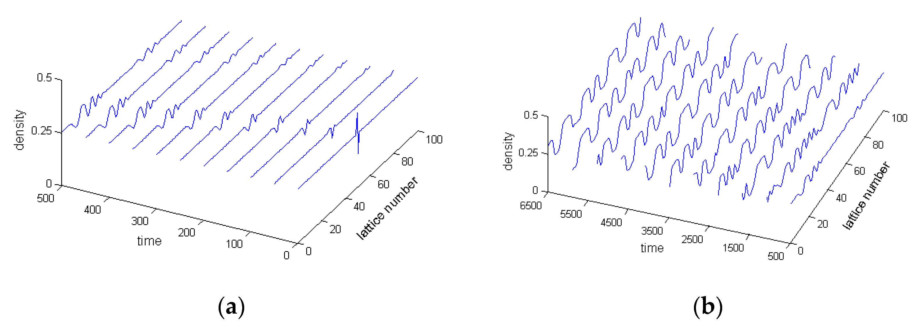
Figure 1 exhibits the traffic wave-developing process of the new model without variable delay and feedback control information. Figure 1a is the traffic wave-developing pattern in the first t = 500 time step and Figure 1b denotes the traffic wave-developing pattern after t = 500 time step. In Figure 1, we can see that the perturbation will cause the initial stable traffic flow to become unstable. In a short simulation time, the traffic flow will evolve into a local perturbation, as shown in Figure 1a. As time goes on, the whole traffic system will turn out to be unstable, as shown in Figure 1b, and the unstable traffic flow is consistent with stop-and-go phenomena in real traffic situations.
Similarly, Figure 2 and Figure 3 show the traffic wave-developing process of the new model for different variable delays but without the feedback control. The variable delay in Figure 2 is d ( k ) = round ( 2 + sin ( k ) ) and the variable delay in Figure 3 is d ( k ) = round ( 3 + 2 sin ( k ) ) , where round (   ) is the rounding function. It is clear that the interval of the variable delay in Figure 2 is (1,3) and in Figure 3 is (1,5). From Figure 2 and Figure 3, it is observed that the original traffic still becomes unstable under the perturbation. However, by comparing the scale of the oscillation of the traffic wave in Figure 1 and Figure 2, it is observed that the vibration level of unstable traffic in Figure 2 is more severe than that in Figure 1. This represents that the variable delay can lower the stable level of the traffic system and lead to a worse traffic jam. Further, from Figure 2 and Figure 3, it is found that the unstable situation of traffic flow becomes more serious when the interval of the variable delay is longer. From Figure 1, Figure 2 and Figure 3, we can conclude that the traffic system is more likely to evolve into a traffic jam when variable delay is considered, and a longer interval of variable delay can cause greater traffic congestion.
Further, Figure 4 and Figure 5 show the traffic flow generation process of the new model when variable delay and feedback control are both taken into account. The variable delay in Figure 4 and Figure 5 is d ( k ) = round ( 3 + 2 sin ( k ) ) , and the feedback control gain in Figure 4 is β = 0.03 and in Figure 5 is β = 0.06 . In Figure 4, the fluctuation in traffic still appears, but the amplitude of the traffic wave is smaller than that in Figure 3. Additionally, when β increased to β = 0.06 , it can be seen in Figure 5 that the initial disturbance disappears in the traffic evolution process, and the traffic jam has been suppressed. This makes clear that the feedback control information of flux difference of the target lattice and its two preceding lattices can elevate traffic stability, and a more significant feedback control gain can ensure a more stable degree of traffic.
Corresponding to Figure 1, Figure 2, Figure 3, Figure 4 and Figure 5, Figure 6 shows the traffic wave sketch of lattice j = 45 from t = 0 to t = 6000 time step, in which Figure 6a corresponds to β = 0 and d ( k ) = 0 , Figure 6b corresponds to β = 0 and d ( k ) = round ( 2 + sin ( k ) ) , Figure 6c corresponds to d ( k ) = round ( 3 + 2 sin ( k ) ) and β = 0 , Figure 6d corresponds to d ( k ) = round ( 3 + 2 sin ( k ) ) and β = 0.03 and Figure 6e corresponds to d ( k ) = round ( 3 + 2 sin ( k ) ) and β = 0.06 , respectively. Figure 6 shows that the range of the traffic wave is enlarged when the variable delay is taken into account and further enlarged when the interval of the variable delay is increased. Moreover, the seriousness of the traffic jam has been reduced gradually when the feedback control information is considered, and the stabilizing effect on traffic flow for a bigger feedback control weighting coefficient is much more obvious.
Further, Figure 7 compares the traffic wave evolution sketch of the model with variable delay and constant delay. The density wave sketches are obtained for lattice j = 45 from t = 0 to t = 6000 when control gain β is set as β = 0 . Figure 7a shows the result when variable delay is considered, and the variable delay is d ( k ) = round ( 3 + 2 sin ( k ) ) . Figure 7b,c corresponds to the traffic wave sketch when d ( k ) is set as constant delays of d 1 ( k ) = 1 and d 2 ( k ) = 5 . It is clear that d 1 ( k ) and d 2 ( k ) are the constant upper bound and lower bound of variable delay d ( k ) = round ( 3 + 2 sin ( k ) ) . From Figure 7, it is observed that the traffic flow finally turns out to be unstable. The scale of the unstable density wave in Figure 7a is also between the density wave scales in Figure 7b,c. This represents that the unstable level of traffic flow caused by the variable delay is stronger than the fluctuation degree of traffic flow caused by the constant upper bound of the variable delay. Nonetheless, it is weaker than the fluctuation level in traffic flow caused by the constant lower bound of the variable delay.

5. Conclusions

In this paper, a novel time-discrete macro traffic system constructed based on a lattice hydrodynamic traffic model is introduced. Through this new model, the influence of variable delay and feedback control strategy on traffic flow is explored, and a stable condition is provided to ensure the stability of the new model with respect to variable delay and feedback control parameters. Furthermore, the impact of variable delay and feedback control on traffic stability is exhibited with a simulation. We observed that variable delay can deteriorate traffic jams, and feedback control information can significantly promote a stable standard of traffic. In addition, the seriousness of traffic jams caused by the variable delay is between the congestion level caused by the constant lower bound of the variable delay and the congestion level caused by the constant upper bound of the variable delay. Nevertheless, the control signal introduced in this paper is restricted to the current lattice’s two preceding lattices. Using communication technologies for vehicle-to-vehicle or vehicle-to-infrastructure, the traffic information for the current lattice can also be acquired at further distances. The influence of traffic information far ahead of the current lattice on the performance of traffic systems will be studied in future works.

Author Contributions

S.J.: Methodology, Writing; G.Z.: Investigation, Supervision, Writing; Y.Z.: Methodology, Software; D.-B.P.: Investigation, Writing; W.-Z.X.: Software, Writing. All authors have read and agreed to the published version of the manuscript.

Funding

This research was sponsored by the National Key Research and Development Program of China, Grant Number 2018YFB2004104 and 2018YFB2004103, and the Natural Science Foundation of Chongqing, China, Grant Number cstc2019jcyj-msxmX0265.

Conflicts of Interest

The authors declare no conflict of interest.

References

  1. Bando, M.; Hasebe, K.; Nakayama, A.; Shibata, A.; Sugiyama, Y. Dynamics model of traffic congestion and numerical simulation. Phys. Rev. E 1995, 51, 1035–1042. [Google Scholar] [CrossRef] [PubMed]
  2. Jiao, S.Y.; Zhang, S.R.; Zhou, B.; Zhang, L.; Xue, L.Y. Dynamic performance and safety analysis of car-following models considering collision sensitivity. Physica A 2021, 564, 125504. [Google Scholar] [CrossRef]
  3. Lee, S.; Ngoduy, D.; Keyvan-Ekbatani, M. Integrated deep learning and stochastic car-following model for traffic dynamics on multi-lane freeways. Transp. Res. Part C 2019, 106, 360–377. [Google Scholar] [CrossRef]
  4. Tordeux, A.; Roussignol, M.; Lassarre, S. Linear stability analysis of first-order delayed car-following models on a ring. Phys. Rev. E 2012, 86, 036207. [Google Scholar] [CrossRef]
  5. Treiber, M.; Kanagaraj, V. Comparing numerical integration schemes for time-continuous car-following models. Physica A 2015, 419, 183–195. [Google Scholar] [CrossRef] [Green Version]
  6. Chen, X.Y.; Sun, J.; Ma, Z.; Sun, J.; Zheng, Z.D. Investigating the long- and short-term driving characteristics and incorporating them into car-following models. Transp. Res. Part C 2020, 117, 102698. [Google Scholar] [CrossRef]
  7. Treiber, M.; Kesting, A.; Helbing, D. Delays, inaccuracies and anticipation in microscopic traffic models. Physica A 2006, 360, 71–88. [Google Scholar] [CrossRef]
  8. Payne, H.J. Models of Freeway Traffic and Control; Simulation Council Incorporated: La Jolla, CA, USA, 1971; pp. 51–61. [Google Scholar]
  9. Aw, A.; Rascle, M. Resurrection of “second order” models of traffic flow. SIAM J. Appl. Math. 2000, 6, 916–938. [Google Scholar] [CrossRef]
  10. Nagatani, T. Modified KdV equation for jamming transition in the continuum models of traffic. Physica A 1998, 261, 599–607. [Google Scholar] [CrossRef]
  11. Khan, Z.H.; Gulliver, T.A. A macro traffic model based on transition velocities. J. Comput. Sci. 2020, 43, 101131. [Google Scholar] [CrossRef]
  12. Jiang, R.; Wu, Q.S. Extended speed gradient model for mixed traffic. Transp. Res. Rec. 2004, 1883, 78–84. [Google Scholar] [CrossRef]
  13. Wang, Q.Y.; Cheng, R.J.; Ge, H.X. A new lattice hydrodynamic model accounting for the traffic interruption probability on a gradient highway. Phys. Lett. A 2019, 383, 1879–1887. [Google Scholar] [CrossRef]
  14. Kesting, A.; Treiber, M.; Helbing, D. Enhanced intelligent driver model to access the impact of driving strategies on traffic capacity. Philos. Trans. R. Soc. A 2010, 368, 4585–4605. [Google Scholar] [CrossRef] [Green Version]
  15. Tian, J.F.; Jiang, R.; Li, G.; Treiber, M.; Jia, B.; Zhu, C.Q. Improved 2D intelligent driver model in the framework of three-phase traffic theory simulating synchronized flow and concave growth pattern of traffic oscillations. Transp. Res. Part F 2016, 41, 55–65. [Google Scholar] [CrossRef]
  16. Treiber, M.; Kesting, A. The intelligent driver model with stochasticity-New insights into traffic flow oscillations. Transp. Res. Part B 2018, 117, 613–623. [Google Scholar] [CrossRef] [Green Version]
  17. Nagel, K.; Schreckenberg, M. A cellular automaton model for freeway traffic. J. Phys. I 1992, 2, 2221–2229. [Google Scholar] [CrossRef]
  18. Tian, J.F.; Zhu, C.Q.; Jiang, R.; Treiber, M. Review of the cellular automata models for reproducing synchronized traffic flow. Transp. A 2021, 17, 766–800. [Google Scholar]
  19. Zhao, H.T.; Liu, X.R.; Chen, X.X.; Lu, J.C. Cellular automata model for traffic flow at intersections in internet of vehicles. Physica A 2018, 494, 40–51. [Google Scholar] [CrossRef]
  20. Daganzo, C.F. The cell transmission model: A dynamic representation of highway traffic consistent with the hydrodynamic theory. Transp. Res. Part B 1994, 28, 269–287. [Google Scholar] [CrossRef]
  21. Zhong, R.X.; Sumalee, A.; Pan, T.L.; Lam, W.K. Stochastic cell transmission model for traffic network with demand and supply uncertainties. Transp. A 2013, 9, 567–602. [Google Scholar] [CrossRef]
  22. Shirke, C.; Bhaskar, A.; Chung, E. Macro modelling of arterial traffic: An extension to the cell transmission model. Transp. Res. Part C 2019, 105, 54–80. [Google Scholar] [CrossRef]
  23. Yu, L.; Shi, Z.K.; Li, T. A new car-following model with two delays. Phys. Lett. A 2014, 378, 348–357. [Google Scholar] [CrossRef]
  24. Li, S.K.; Yang, L.X.; Gao, Z.Y.; Li, K.P. Stabilization strategies of a general nonlinear car-following model with varying reaction-time delay of the drivers. ISA Trans. 2014, 53, 1739–1745. [Google Scholar] [CrossRef]
  25. Kang, Y.R.; Sun, D.H. Lattice hydrodynamic traffic flow model with explicit drivers’ physical delay. Nonlinear Dyn. 2013, 71, 531. [Google Scholar] [CrossRef]
  26. Zhang, G. Study on varying time delay on traffic stability in a novel lattice hydrodynamic model. Physica A 2018, 505, 1103. [Google Scholar] [CrossRef]
  27. McCartney, M. A discrete time car following model and the bi-parameter logistic map. Commun. Nonlinear Sci. Numer. Simul. 2009, 14, 233–243. [Google Scholar] [CrossRef]
  28. Zhu, W.X.; Zhang, L.D. Discrete car-following model and its feedback control scheme. Asian J. Control 2020, 22, 182–191. [Google Scholar] [CrossRef]
  29. Wu, M.; He, Y.; She, J.H. Robust Control of Time-Delay Systems–The LMI Method; Science Press: Beijing, China, 2008. [Google Scholar]
Figure 1. Traffic wave-developing process of the new model when β = 0 and d ( k ) = 0 , in which (a) in the first t = 500 time step, (b) after t = 500 time step.
Electronics 10 02346 g001
Figure 2. Traffic wave-developing process of the new model when β = 0 and d ( k ) = round ( 2 + sin ( k ) ) , in which (a) in the first t = 500 time step, (b) after t = 500 time step.
Electronics 10 02346 g002
Figure 3. Traffic wave-developing process of the new model when β = 0 and d ( k ) = round ( 3 + 2 sin ( k ) ) , in which (a) in the first t = 500 time step, (b) after t = 500 time step.
Electronics 10 02346 g003
Figure 4. Traffic wave-developing process of the new model when β = 0.03 and d ( k ) = round ( 3 + 2 sin ( k ) ) , in which (a) in the first t = 500 time step, (b) after t = 500 time step.
Electronics 10 02346 g004
Figure 5. Traffic wave-developing process of the new model when β = 0.06 and d ( k ) = round ( 3 + 2 sin ( k ) ) , in which (a) in the first t = 500 time step, (b) after t = 500 time step.
Electronics 10 02346 g005
Figure 6. Traffic wave sketch of lattice j = 45 for different d ( k ) and β, in which (a) β = 0 and d ( k ) = 0 , (b) β = 0 and d ( k ) = round ( 2 + sin ( k ) ) , (c) β = 0 and d ( k ) = round ( 3 + 2 sin ( k ) ) , (d) β = 0.03 and d ( k ) = round ( 3 + 2 sin ( k ) ) , (e) β = 0.06 and d ( k ) = round ( 3 + 2 sin ( k ) ) .
Electronics 10 02346 g006
Figure 7. Traffic wave sketch of lattice j = 45 for variable delay and constant delay, in which (a) d ( k ) = round ( 3 + 2 sin ( k ) ) , (b) d ( k ) = 1 and (c) d ( k ) = 5 .
Electronics 10 02346 g007
Publisher’s Note: MDPI stays neutral with regard to jurisdictional claims in published maps and institutional affiliations.

