Optimization of Energy Consumption Based on Traffic Light Constraints and Dynamic Programming

Abstract

Traffic lights are an important part of urban roads. They improve traffic conditions but bring about a limitation of driving speed in the space–time domain for vehicles. In this paper, a traffic light model based on a vehicle–road cooperative system is built. The model provides the vehicle with speed constraints when passing the green light in the time–space domain. A global-optimization-based energy management strategy based on dynamic programming (DP) is constructed with the constraints. The simulations are performed for two driving situations of different signal phases with the electric vehicle driven by a single power source. Compared with the traditional fixed speed driving strategy and green light optimal speed advisory (GLOSA) system, the energy management strategy proposed in this paper is able to control operating points of the motor to be distributed in more efficiency areas. A higher economy is achieved from simulation results.

1. Introduction

In recent years, the deterioration of the environment and the shortage of oil resources have brought serious challenges to the automotive industry [1]. Rational planning of vehicle energy management strategies to reduce energy consumption has great importance and necessity. As they play an indispensable role in urban roads, traffic lights play an important part in improving traffic management and road utilization rates. However, red traffic signals can cause vehicles to changes their driving conditions. Braking and acceleration will further increase the energy consumption of the vehicle. When traffic light information is available, vehicles can take more appropriate control strategies in advance to achieve adaptive control to reduce energy consumption [2].

The commonly used methods for traffic light information acquisition can be divided into two categories. One is the information communication method using V2I. The other is the image recognition method based on machine vision.

With the development of intelligent transportation system (ITS), vehicle-to-infrastructure (V2I) technology has been used in a large number of applications to solve road traffic congestion, environmental protection and safety [3]. In the context, vehicles are allowed to interact with neighboring infrastructure through communication protocols such as DSRC [4], LTE [5], 5G [6], etc. Drivers can take rational control through crossroads in a speed-guided manner to reduce vehicle delays and unnecessary stops. The machine vision-based image recognition method uses the vehicle’s own sensors to collect traffic light images by means of color recognition or image classification. Li et al. preprocessed the collected nighttime traffic light images to achieve recognition based on regional pixel information and template matching. The experimental results showed that the recognition accuracy of the algorithm is higher than other methods [7]. Wang et al. proposed a real-time traffic light recognition system based on HDR imaging and deep learning. Experimental results show that the performance of the proposed traffic light recognition outperforms the current deep learning target detector using only bright images [8]. Kim et al. proposed a two-stage traffic light recognition method based on deep learning. Simulation results show that the proposed traffic light recognition method outperforms the traditional Faster R-CNN in terms of recognition performance [9]. Additional lights may appear within the camera’s field of view, which brings great difficulties to image recognition. In addition, the image recognition method based on machine vision can only capture the current state of the traffic light. For traffic lights without countdown, the time of the remaining signal is usually unknown. All these factors limit the use of the recognition method.

When utilizing traffic light information for vehicle control, it is necessary to construct an energy management strategy for the vehicle. The energy management strategy is a key technology in the design and development of vehicle control systems, which directly affects the dynamic performance and economic performance of the vehicle.

The control strategy can be formulated as a rule-based energy management strategy or an optimization-based energy management strategy [10]. The rule-based energy management strategy utilizes component characteristics as the basis for energy allocation and control of each power component with the aid of engineering experience and expert knowledge. Kim et al. proposed an advanced series hybrid bus power distribution strategy by combining a thermostat strategy and a power follower strategy. The economy of the proposed strategy was increased by 7.78% and 11.28% compared with thermostat strategy and power follower strategy, respectively [11]. Jeoung et al. proposed a rule-based control method for parallel type 2 hybrid vehicles (P2 hybrids). The results show that the rule-based concept achieved higher fuel efficiency [12]. Rule-based energy management strategies rely on expert knowledge. When combined with complex and variable traffic information, rules need to be established for multiple driving conditions, which results in increasing the time cost of the development of the energy management strategy.

Optimization-based energy management strategies are divided into global-optimization-based energy management strategies and instantaneous-optimization-based energy management strategies [10]. In the terms of global-optimization-based energy management strategies, dynamic programming (DP) achieves the best control effect for a given task. Liu et al. used DP algorithm to solve the global optimal control strategy under different driving cycles. The results of simulation show that the DP had significant advantages over rule-based control strategy in fuel economy improvement [13]. Hu et al. designed DP economical cruise control algorithms under discrete distance strategy, which reduced energy consumption by 21.6% at constant driving speeds [14]. DP requires prior information and a large number of calculations. It is difficult to apply to strategy development for actual vehicle driving. So the result of it is often used as a benchmark for comparison with other energy management strategies. In the terms of instantaneous-optimization-based energy management strategies, Rezaei et al. investigated an energy management strategy based on equivalent consumption minimization strategy (ECMS) whose optimal equivalent factor was determined by giving the full trajectory of the driver demanded power. The proposed strategy improves the fuel economy by 7% compared with traditional ECMS [15]. Keller et al. proposed a hierarchical-level energy management strategy based on nonlinear MPC. After simulation, the proposed strategy achieved a longer predicted horizon and reduced fuel consumption [16]. The practicality and control effectiveness of instantaneous-optimization-based energy management strategies are between rule-based energy management strategies and global-optimization-based energy management strategies. If it does not reduce the amount of computation and achieve a sufficient optimization effect, the applicability of the transient optimization strategy will be degraded.

In the existing studies, there are many scholars who combine signal information and vehicle energy consumption to design control strategies. Altan et al. divided traffic tasks into four categories, namely cruise, acceleration, deceleration to stop and eco-slide. The proposed control logic tries to minimize the vehicle’s acceleration/deceleration before the intersection, so that the vehicle can pass the intersection with the target speed that is closest to its initial speed. The results show an average saving of about 17% in fuel consumption [17]. Wang et al. developed a cooperative eco-driving system to improve the energy efficiency of signalized intersections through connected and automated vehicle technology. A microscopic traffic simulation network was constructed in VISSIM. The results showed a 7% reduction in energy consumption and a 59% reduction in pollutant emissions [18]. Yu et al. proposed a consensus and optimal speed advisory model (SAM) for signalized intersections in mixed traffic scenarios with the aim of improving vehicle economy and safety. Numerical simulation results show that the proposed method can improve the safety and fuel economy of mixed traffic on signal-controlled highways [19]. Currently, attention is being paid to green light optimal speed advisory (GLOSA) systems, which are seen as one of the key solutions to such problems. Suzuki et al. validated GLOSA to achieve higher fuel efficiency and lower CO₂ [20]. Most of the studies over-simplify specific driving situations when constructing traffic light models. In particular, the proposed traffic strategies do not consider all possible speeds at each moment. Such a simplification undoubtedly reduces the optimization problem’s search space.

In this context, a traffic light model is constructed based on standardized map information and signal phase and timing (SPaT) messages obtained by V2I communication. Combined with the constraints provided by the traffic light model, a DP-based energy management strategy is developed to adjust the longitudinal control of the vehicle to reduce the number of stops and improve its economy. In order to avoid the simulation results being affected by changes in power distribution between multiple components, this paper uses an electric vehicle (EV) for simulation to verify the control effect.

The innovations of this paper are as follows.

• The speed constraints at discrete moments are used to realize an arbitrary dynamic process, which simplifies the complexity of modeling and provides a larger space for the subsequent energy management optimization to find the optimal control solution;
• The optimization problem is constructed by the combining traffic light model and an energy management strategy. The vehicle’s economy is improved under the premise of passing on a green light;
• A multisignal, multiscenario passing task with random initial phase is constructed to validate the DP-based energy management strategy.

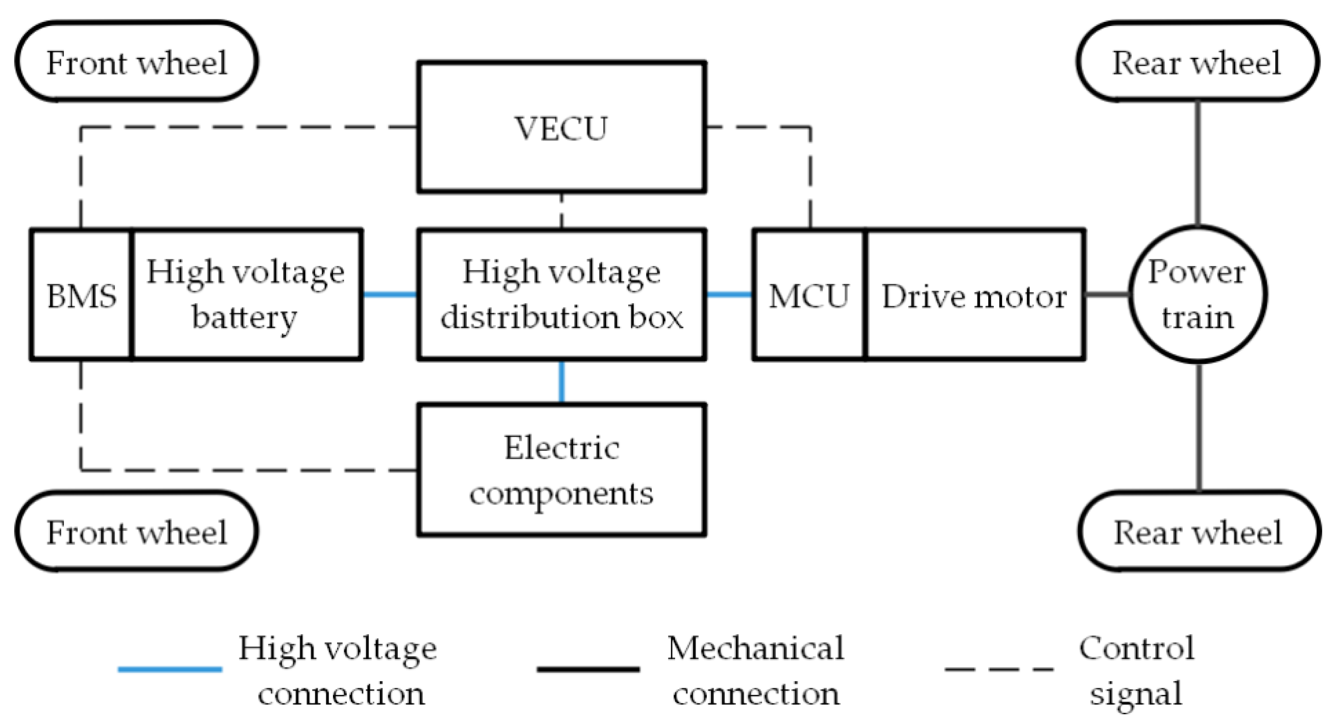
The remainder of this paper is structured as follows. Section 2 introduces the vehicle model. Section 3 introduces the traffic signal model. Section 4 introduces the DP-based energy management strategies. Section 5 shows the simulation results. Section 6 concludes the paper.

2. Vehicle Model

Throughout the process of optimizing a vehicle passing through a signalized intersection, it is inevitable that one must adjust the vehicle’s passing speed to avoid stopping and restarting in order to improve the vehicle’s economy. The optimization of energy consumption may be caused by a change in the power distribution relationship and not by a more economical vehicle speed. In conclusion, a multipower vehicle cannot accurately reflect the optimization effect of speed planning. Therefore, this paper takes the EV with a single power source as the research object and builds a vehicle model based on 2020b version Matlab/Simulink platform.

2.1. Vehicle Parameters

The configuration of EV is shown in Figure 1. The whole vehicle power unit adopts permanent magnet synchronous motor which is controlled by motor control unit (MCU) and transmits the power to the rear wheels through power train [21]. The whole vehicle energy device adopts lithium iron phosphate battery which is controlled by a battery management system (BMS) and provides electric power for the motor and electric components through the high voltage distribution box [22]. The vehicle electronic control unit (VECU) receives control instructions from the accelerator and brake pedals, gives the correct control signal to the high voltage distribution box to control the direction of power flow, and also controls the regenerative braking and electronic accessories together with the energy management system [23]. The detailed parameters of the studied vehicle are shown in

Table 1. Vehicle and component parameters in the studied vehicle.

Component	Parameter	Value	Unit
Vehicle	Vehicle weight	1200	kg
	Tire radius	0.3	m
	Frontal area	3	m2
	Drag coefficient	0.4	/
	Final drive ratio	6	/
Motor	Maximum torque	307	Nm
	Maximum power	126	kW
	Rated power	60	kW
	Maximum RPM	12,584	r/min
	Inertia	0.1	kg·m2
Battery	Rated capacity	24	kWh
	Rated voltage	366	V

.

2.2. Vehicle Dynamic Model

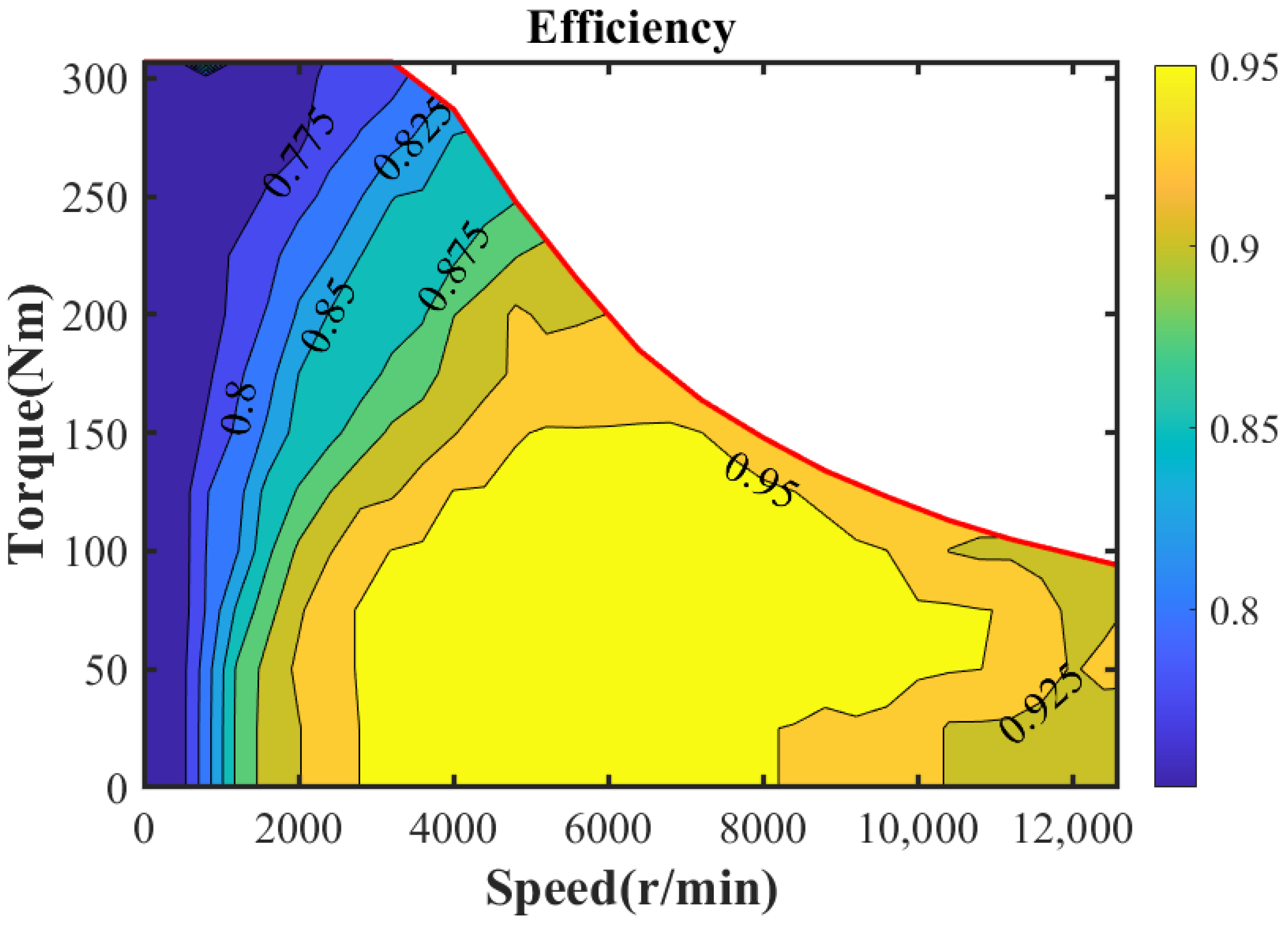
The dynamics of the vehicle are determined by the longitudinal forces [24]. There are various external forces acting in the longitudinal direction while the vehicle is in motion, including the driving force and other driving resistances. The vehicle driving balance equation is described as follows [25]:

$$F_{trac}=mgf\cos \theta +mg\sin \theta +\frac{C_{D}A{v}^2}{21.15}+\sigma m\frac{dv}{dt}$$

(1)

where $m$ is the vehicle mass, $g$ is acceleration of gravity, $f$ is the coefficient of rolling resistance, $\theta$ is the road slope, $C_D$ is the air resistance coefficient, $A$ is the frontal area and $\sigma$ is the rotational mass conversion factor.

2.3. Motor Model

The EV studied in this paper is driven by a permanent magnet synchronous motor, whose efficiency map at rated power is shown in Figure 2. The output torque and efficiency of the motor are described in Equations (2) and (3), respectively.

$$T_{mot}=f_T(n_{mot},{\alpha }_{mot})$$

(2)

$${\eta }_{mot}=f_{\eta }({\mathrm{n}}_{mot},T_{mot})$$

(3)

where $n_{mot}$ is motor speed, $\alpha$ is motor load and takes the value of $[-1,1]$, $T_{mot}$ is motor torque and ${\eta }_{mot}$ is motor energy conversion efficiency. Electrical power is converted into mechanical power when the motor is driven. The conversion direction is reversed when the vehicle undergoes regenerative braking. The formula for calculating the battery output power is described in the following equation:

$$P_e=\{\begin{array}{cc}\frac{T_{mot}{n}_{mot}}{{\eta }_{mot}}& T_{mot}\ge 0\\ T_{mot}{n}_{mot}{\eta }_{mot}& T_{mot}<0\end{array}$$

(4)

where $P_e$ is the battery output power.

2.4. Battery Model

In this paper, a Rint model is used to describe the battery performance. The model consists of an ideal voltage source and an internal resistance in series. The mathematical expression of its working characteristics is shown in the following equation [26]:

$$R_0\cdot I=U_{oc}-U_L$$

(5)

where $U_{oc}$ is open circuit voltage of battery, $U_L$ is the terminal voltage at the positive and negative ends of battery, $R_0$ is the ohmic internal resistance of battery, and $I$ is the current in the circuit. The current integration method is used to effectively estimate the remaining energy by integrating the battery charging current and discharging current in real time to obtain the state of charge (SOC) variation. The variation curve of SOC with time is calculated from the initial $SO{C}_0$ [27]. The formula is as follows:

$$SOC=SO{C}_0-{\displaystyle \int \frac{\mathrm{Idt}}{Q(I)}}$$

(6)

where $Q(I)$ is the ampere-time capacity of the battery corresponding to the rate of current changes and $SO{C}_0$ is the initial value of $SOC$.

3. Traffic Light Model

In order to consider different approaches of vehicles, this paper establishes a traffic light model that is applicable in all driving conditions. The phase information, timing information and localization information of traffic lights are received by the model. Combining the vehicle positioning from GPS and the city map from cloud server, the traffic light model outputs the speed constraint that ensures vehicles pass the intersection during the green light. The model provides constraints for the subsequent construction of an optimization-based energy management strategy that can be used to improve economy.

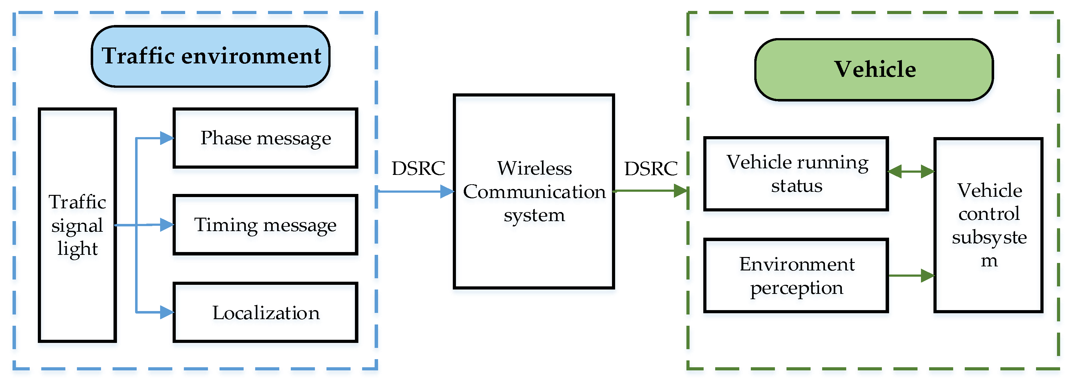
3.1. Vehicle–Road Collaborative System

V2I is essential for the successful deployment and operation of intelligent transportation systems [28]. In this paper, DSRC wireless communication technology is used for V2I messaging, which provides high speed data transmission, ensures low latency of the communication link and guarantees the reliability of the system.

The traffic signal information is divided into timing information, phase information and localization information. The timing information includes the duration of each color of the traffic light. The timing information of all colors constitute a cycle of the traffic light. The phase information refers to the moment of the current color in a cycle. The localization information is combined with GPS to determine the distance to the next intersection. The illustration of the cooperative vehicle infrastructure system framework is shown in Figure 3. The system transmits the traffic signal information to the wireless communication system through the DSRC specialized communication channel. The signal receiver on the vehicle end sends the received information to the data processing unit. The data processing unit combines the current running status of the vehicle and the traffic light information to propose constraints on the vehicle speed. Finally, a suitable energy management strategy is set. Since this paper does not consider the real-time adjustment of signal information, it does not involve the information transmitting proceeding from the vehicle to the traffic light.

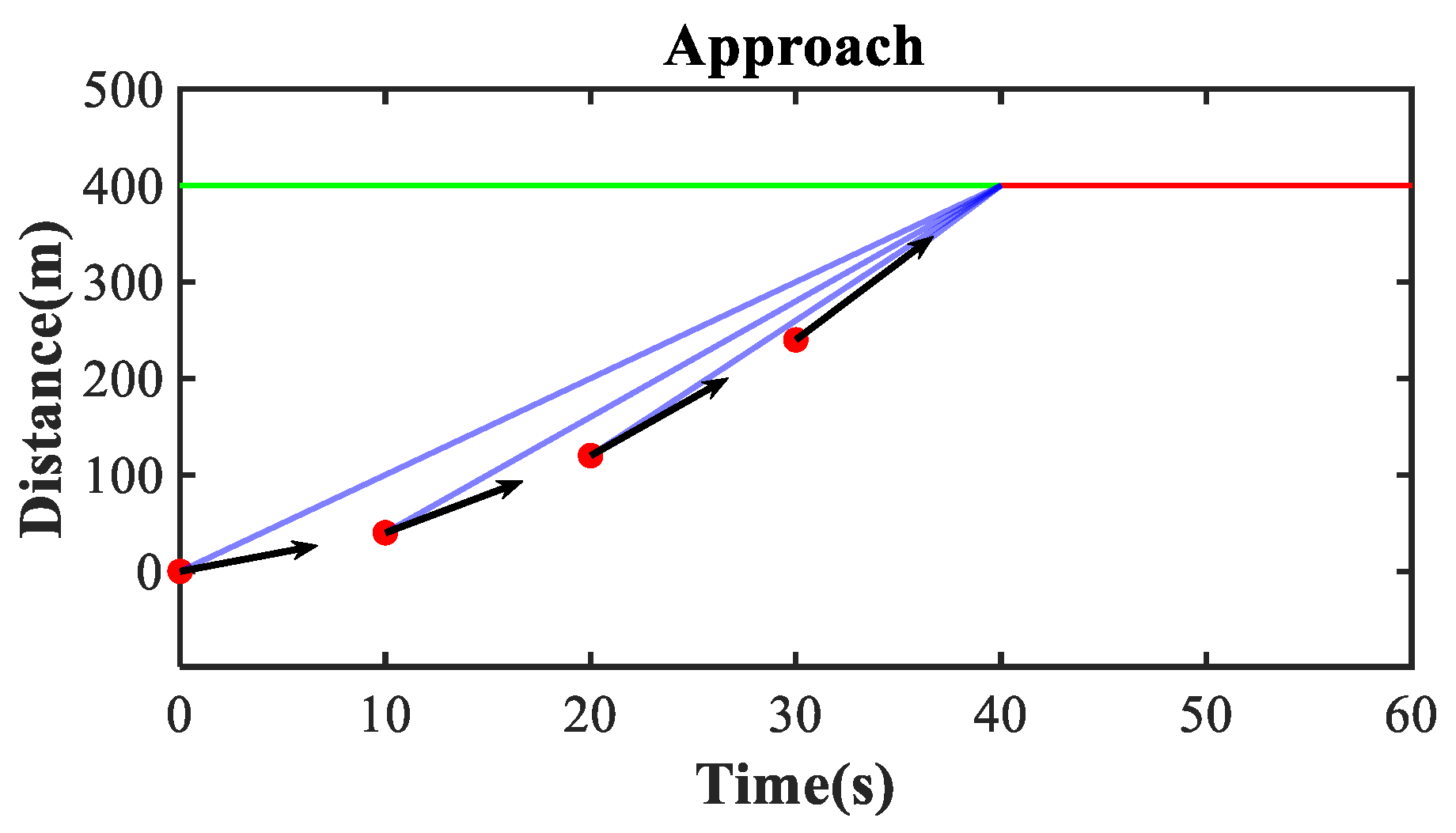
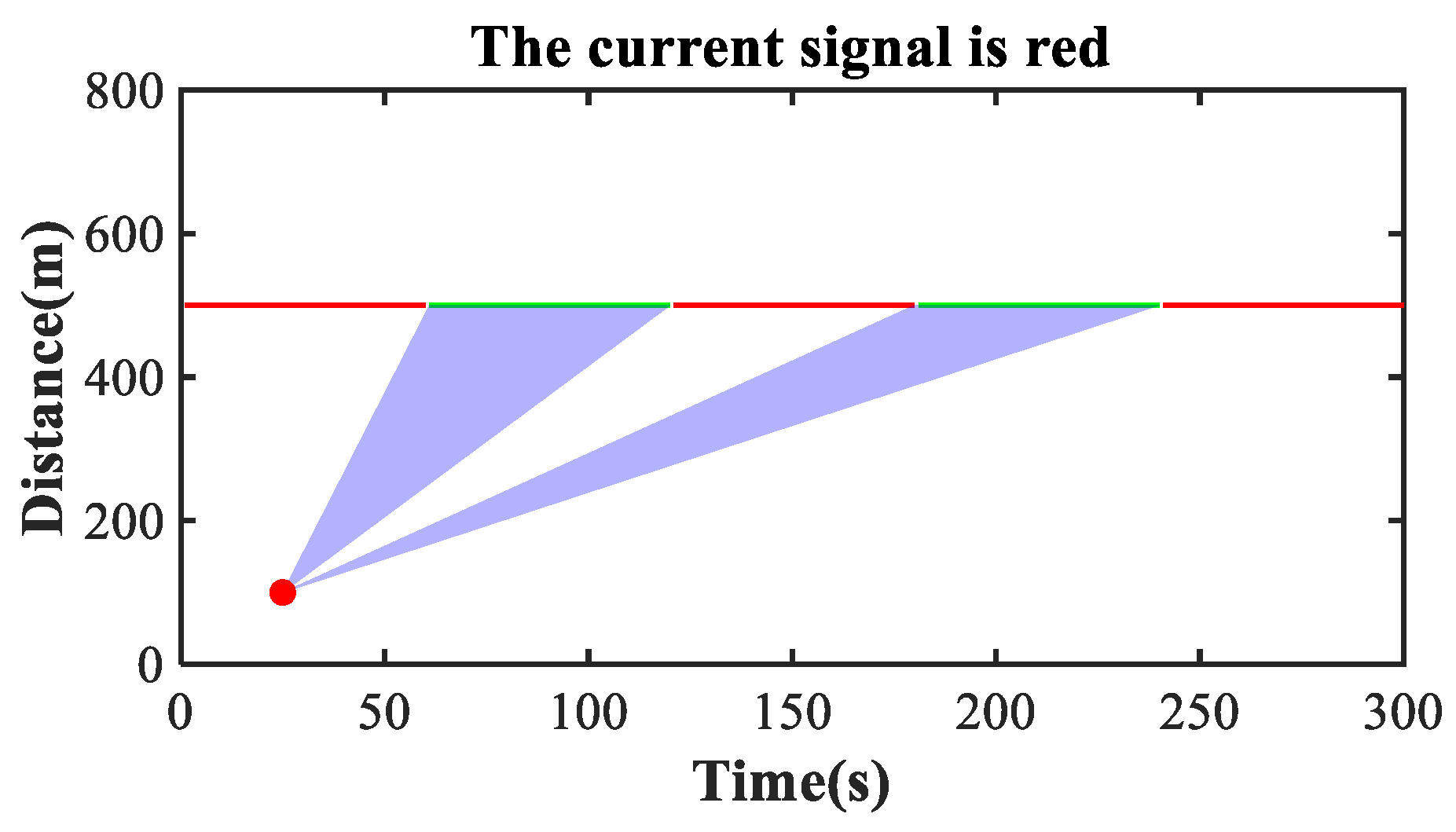
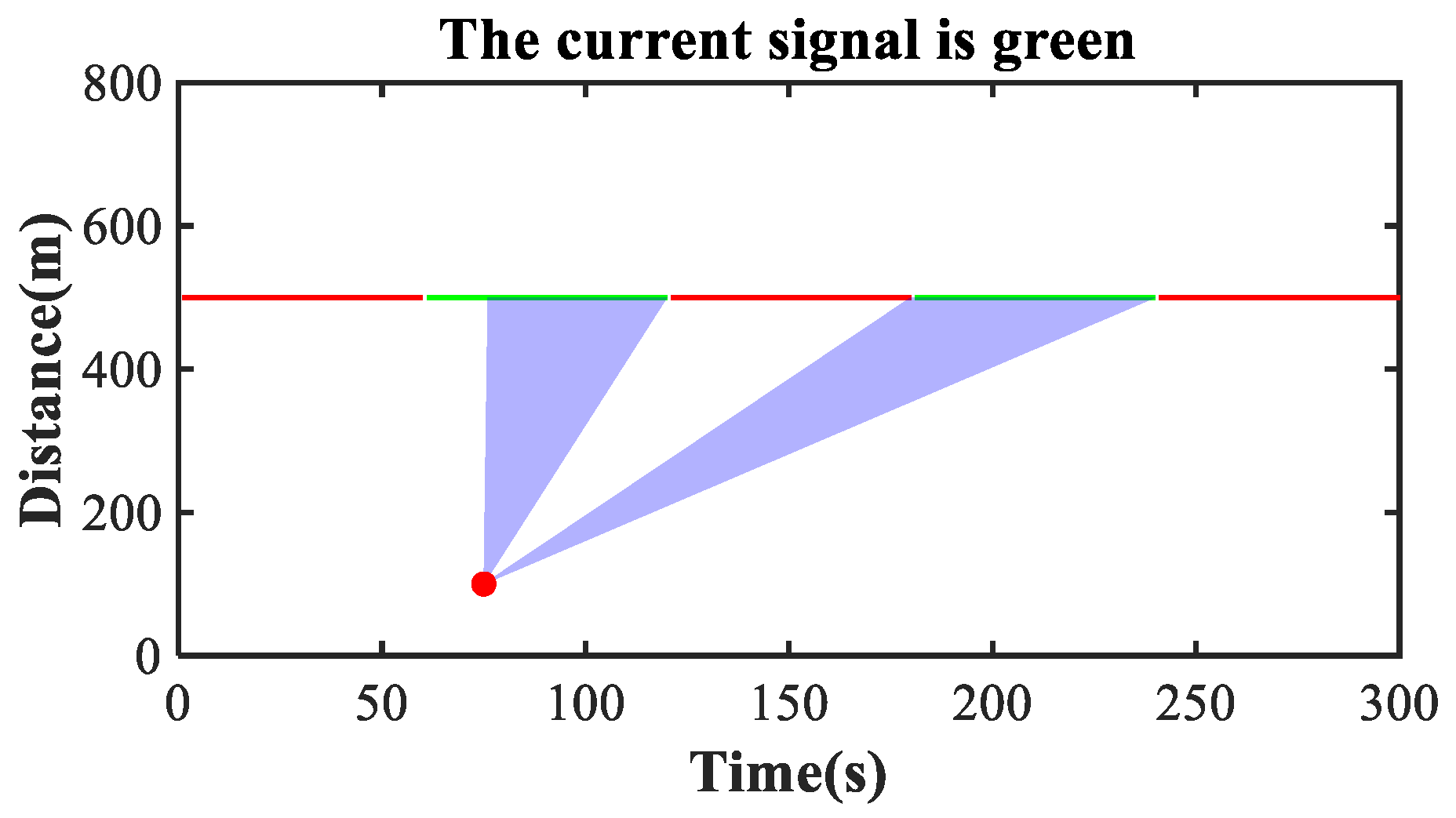
3.2. Traffic Constraints

In order to facilitate the analysis and sharpen the problem, the following rationalization assumptions are made in this paper.

• The time of communication transmission is ignored when the traffic information is transmitted between vehicle end and road end.
• Assume that the vehicle always drives along a straight line, ignoring steering driving conditions.
• After interference from other vehicles, this is equivalent to re-specifying the initial vehicle state and solving a new optimization problem for the instantaneous-optimization-based energy management strategy. This paper studies a complete optimization process, assuming that the vehicle is not affected by other vehicles.
• Simplify the red-green-yellow signal to red-green signal for partial security assumption. The color of the traffic light is considered to be red during the period of yellow.

If the entire process of the vehicle passing is considered, there will be an infinite combination of vehicle speed and acceleration levels for a given driving situation, which will pose applicability and practicality challenges for modeling. Therefore, in order to complete the vehicle path planning and energy optimization simultaneously, this paper puts forward the following requirements for the traffic light model based on the optimized control strategy.

• The input information of the traffic light model should be consistent with the data that can be provided by the cooperative vehicle infrastructure system.
• The proposed model should be applicable to traffic lights with different phases and different distances.
• The traffic light model should give an indicator which provides constraints for subsequent energy management optimization.
• Control actions should be implemented by energy management strategies rather than the traffic light model.

Constructing the timing model of traffic lights using sine function. The formula is described as follows:

$$L\left(t\right)=sin(\omega t+\phi )+h$$

(7)

where $\omega$, $\phi$, $h$ is the parameter of the trigonometric function, $w>0$, $\phi \in [0,2\pi ]$, $h\in (-1,1)$ and $L(t)$ represents the lighted situation of the traffic light, respectively. If $L(t)\ge 0$ means red light at moment $t$. If $L(t)<0$ means green light at moment $t$. The following equation is used to represent the spatial distance of the optimization task.

$$D(d)=D_i-d$$

(8)

where $d$ is the current position of the vehicle, $D_i$ indicates the position of the next traffic light and $D(d)$ is the distance from the current vehicle position to the next traffic light position.

The more effective way to design the passing speed is to discretize the passing process and constrain the speed at each moment. By making multiple comparisons at discrete moments, the vehicle acceleration is adjusted so that the vehicle can pass through the intersection within the green light. An example diagram for replacing the dynamic adjustment process with a discrete method is shown in Figure 4. The horizontal line represents a traffic light 400 m away from the starting position. The color of the horizontal line represents the color of the traffic light that changes with time. The red dots represent the position of the vehicle at different moments. The slope of the black arrow represents the speed of the vehicle at the current position. The blue line is the average speed required to ensure that the vehicle passes before the end of the green light. In Figure 4, at the initial moment, the vehicle speed is slow and the black arrow is below the blue line. If the vehicle continues to drive at its current speed, it will not be able to pass the interaction before the end of the current green light. The vehicle begins to accelerate gradually until the black arrow coincides with the blue line at 30 s. The vehicle will be able to cross the intersection before the end of the green light by maintaining this speed. In the example only the velocity magnitudes of four moments are given. During the time other than these four moments, the vehicle travel process can be an arbitrary and reasonably complex acceleration and deceleration state. This allows arbitrary dynamic processes to be implemented with speed constraints at discrete moments. The method simplifies the complexity of modeling and also provides a larger optimization search space for subsequent energy management optimization.

The situation is divided into two categories combined with the process of vehicle passage. The first is when the current moment target signal is red, as shown in Figure 5. The second is when the current moment target signal is green, as shown in Figure 6.

In the first category of situation, in order to increase the diversity of the driving process, two subsequent green light periods are chosen to solve the vehicle constraint. As shown in the blue area in Figure 5. The constrained vehicle speed is calculated by the following equation:

$$v_{lim,max}^j=\frac{\omega D(d)}{(2k+2j-1)\pi +\arcsin (h)-\phi -\omega t}$$

(9)

$$v_{lim,min}^j=\frac{\omega D(d)}{(2k+2j)\pi -\arcsin (h)-\phi -\omega t}$$

(10)

$$k=[\frac{wt}{2\pi }]$$

(11)

where $j$ represents that passing at the subsequent $j$th green light on, $[\cdot ]$ is the downward rounding function, $v_{lim,max}^j$ and $v_{lim,min}^j$ is the maximum speed constraint and the minimum speed constraint at the $j$th green light, respectively.

The second category of situation is shown in Figure 6. It is necessary to consider whether the vehicle has time to pass during the current green light period. If it is not in time, then the speed constraint of the subsequent green light needs to be considered. The minimum value of the speed constraint and $k$ are calculated as described in Equations (10) and (11) above. The maximum value of the speed constraint in the second category of situation is described in the following equation:

$$v_{lim,max}^1=\infty$$

(12)

$${\mathrm{v}}_{lim,max}^2=\frac{\omega D\left(d\right)}{(2k+3)\pi +arcsin\left(h\right)-\phi -\omega t}$$

(13)

Ultimately, the constraint results obtained from the traffic light model can be expressed uniformly as the following equation:

$$v_{lim,min}^j\le v\le v_{lim,max}^j$$

(14)

The speed limit must satisfy the relationship of the following equation:

$$v_{lim,min}^2\le v_{lim,max}^2\le v_{lim,min}^1\le v_{lim,max}^1$$

(15)

4. Energy Management Strategy Combined with Traffic Light Model

In this section, the principle of DP algorithm will be introduced first. It will be combined with the traffic light model to construct a global-optimization-based energy management strategy.

4.1. Dynamic Programming Fundamentals

The basic idea of the DP algorithm is to transform a large multistage problem into multiple subproblems of the same type [29]. By solving the optimal solution of the subproblem, the recursive optimization of the original problem is completed. The algorithm is based on the Bellman’s principle of optimality. As a multistage global-optimization-based energy management strategy, regardless of its past states and decisions, the remaining decisions must constitute an optimal substrategy. In short, any part of the substrategies in the optimal policy must also be optimal.

The algorithm is widely used for non-aftereffect problems with deterministic conditions, where decisions are made according to stages. The term “non-aftereffect” means that when the state of the system at a certain stage is known, then the change of the system state after that stage is only related to the current stage and not to all previous stages. Therefore, the solution process of the algorithm starts from the termination stage. The algorithm is solved recursively within the boundary conditions by finding the optimal subproblem for each stage. For each stage of the subproblem, the optimal solution of the previous subproblem is used in the solution process. Thereby, the complexity of the algorithm is reduced and the speed of the algorithm solution is accelerated. For DP algorithms, the following aspects need to be clarified first [30].

• Determine the stage of the optimization problem. Decompose a global optimization problem into several stages of subproblems to be solved. The amount of stages in the solution process is denoted as $k$.
• Determine state variables and control variables for the optimization problem. The state of the system at each stage is described by the state variables. The state variable at stage $k$ is denoted as $x_k$. The decision that acts on the control system to change the system state is described by the control variable. The control variables when the system state is $x_k$ are denoted as $u_k(x_k)$. In the global optimization problem with $k$ stages, there are $k+1$ state variables and $k$ control variables.
• Determine the constraints of the optimization problem. The state variables and control variables of the system often have various constraints, including linear and nonlinear constraints, equation constraints and inequality constraints. Therefore, in the algorithm solution process, the state and control variables must satisfy the constraints of the optimization problem. The optimal control sequence under the global is solved within the allowed range to complete the optimal control of the system.
• Determine the state transfer equation of the optimization problem. The state transfer equation describes the law of the system changing from the state of the current stage to the state of the next stage. By determining the state variables and control variables of the current stage, the state variables of the next stage can be obtained to realize the transfer of the system state.
• Determine the cost function of the optimization problem. The cost function is used to measure the impact of the control system on the system performance in a certain state. The function depends on the current state variables and control variables. At the $kth$ stage, when the system state variable is $x_k$ and the control variable is $u_k$, the cost function is denoted as $J(x_k,u_k)$.

4.2. Global Optimized Energy Management Strategy

In this paper, the energy management task of the EV is transformed into a multistage mathematical problem with traffic constraints. The optimal control under the entire phase is solved computationally using a DP algorithm.

• In this paper, the optimization task is described in terms of driving distance. When the vehicle travels to the target distance, it represents the completion of the whole optimization task. Set the distance interval as 1 m, i.e., $D_s=1$. The ratio of the target distance to the distance interval is taken as the stage of the optimization problem. The stage is calculated as described in the following equation:

  $$N=\frac{D}{D_s}$$

  (16)

  where $D$ is the target distance of the task and N is the stage of the optimization problem.
• The vehicle speed $v$ and travel time $t$ are used as state variables. The motor compensation load rate $\Delta \alpha$ is used as the control variable.

  $$x={[v,t]}^T$$

  (17)

  $$u=\Delta \alpha$$

  (18)

  where $x$ is the state variable and $u$ is the control variable.
• The equation constraint is mainly determined by the vehicle dynamics. That is, the EV is abstracted into a mathematical model and transformed into a mathematical expression. In the driving process, from the perspective of the power balance, the required power is equal to the power generated by overcoming the driving resistance, as described in Equation (19). The power of the motor should be equal to the demanded power of the whole vehicle, as described in Equation (20).

  $$P_{req}=\frac{v}{{\eta }_T}\left(\frac{mgf\cos \alpha }{3600}+\frac{mg\sin \alpha }{3600}+\frac{C_{D}A{v}^2}{76140}+\frac{\sigma m}{3600}\frac{dv}{dt}\right)$$

  (19)

  $$P_m=P_{req}$$

  (20)

  where $P_m$ is power of the motor. The inequality constraint mainly constrains the vehicle components, state variables and control variable. The speed and torque of the motor should be within the range that the motor can provide. The vehicle reversing situation is not considered in this paper, so the vehicle speed should be kept non-negative. In addition, urban roads usually have limits on vehicle speed, so the speed should also be constrained to the traffic regulation. The travel time should be greater than zero and ensure a strict monotonic increment. The absolute value of $\Delta \alpha$ and the actual load rate of the motor should not be greater than 1. The overall inequality constraint is described in the following equation:

  $$\{\begin{array}{c}{n}_{m,min}\le n_m(k)\le n_{m,max}\\ \begin{array}{c}{T}_{m,min}\le T_m(k)\le T_{m,max}\\ 0\le v(k)\le v_{max}\\ 0\le t(k)<t(k+1)\\ -1\le \mathbf{\Delta }\mathbf{\alpha }\le 1\end{array}\\ -1\le \mathbf{\Delta }\mathbf{\alpha }+\mathbf{\alpha }\le 1\end{array}$$

  (21)

  where $k$ is the number of stages, $n_{m,min}$ and $n_{m,max}$ are the minimum and maximum speed of the motor, respectively, $v_{max}$ is the maximum speed of the city road limited by traffic rules which is adopted 80 km/h in this paper and $\alpha$ is the driver-controlled motor load rate.
• Since time is a state variable in this optimization problem and the stage belongs to the spatial domain, it is necessary to use the expression for the spatial domain when the state transfer equation is involved, as described in the following equation:

  $$v(k+1)=\sqrt{v{(k)}^2+2\dot{v}(k)D_s}$$

  (22)

  where $k$ is the current stage, $v$ is the vehicle speed and $\dot{v}$ is the vehicle acceleration. Combining the previous Equation (1), the speed update formula is calculated as described in the following equation:

  $$\dot{v}(k)=\frac{F_{trac}}{\sigma m}-\frac{gf}{\sigma }\cos \theta -\frac{g}{\sigma }\sin \theta -\frac{C_{D}Av{(k)}^2}{21.15\sigma m}$$

  (23)

  $$v(k+1)=\sqrt{v{(k)}^2+\frac{2D_s}{\mathbf{\sigma }m}(F_{trac}-mgf\cos \mathbf{\theta }-mg\sin \mathbf{\theta }-\frac{C_{D}Av{(k)}^2}{21.15})}$$

  (24)
  The time update formula is calculated as described in the following equation:

  $$t(k+1)=t(k)+\frac{2D_s}{v(k)+v(k+1)}$$

  (25)
• In this paper, the cost function of the optimization problem is designed by considering the road speed limit and the motor operating point efficiency, as shown in the following equation:

  $$J={\displaystyle \sum _{k=0}^{N-1}(a{v}_{\cos t}(v)/D(k)+b{\eta }_m(k))}$$

  (26)

  $$v_{\cos t}(k)=\{\begin{array}{cc}0& v(k)\in D_v\\ 1& v(k)\notin D_v\end{array},\hspace{1em}{D}_v=[v_{lim,min}^1,v_{lim,max}^1]\cup [v_{lim,min}^2,v_{lim,max}^2]$$

  (27)

  where $a$ and $b$ are the coefficients, $v_{\cos t}$ is the penalty function of speed and ${\eta }_m$ is the efficiency of the motor. This function allows the vehicle speed to temporarily deviate from the speed constraints of the traffic light model. However, the speed deviation penalty is increased when the vehicle approaches the next traffic light. The complete DP-based global optimal energy management strategy is thus constructed.

The global-optimization-based energy management strategy is thus constructed.

5. Results

The multiintersection passing task is firstly constructed as the optimization task of this paper. Based on the EV model described in Section 2, a DP-based energy management strategy is simulated to complete the passing task and achieve energy consumption optimization. This paper constructs a traditional strategy which controls the vehicle to start and stop at a fixed acceleration and to drive at a fixed speed after starting. Comparisons with the traditional strategy and the GLOSA system are made to test the correctness of the energy management strategy constructed in this paper.

5.1. Build Optimization Task

In this paper, in order to highlight the research problem, only the straight line section is considered. The total length of the simulated section is 3000 m. The number of traffic lights to be passed in the task is five. The distance of each traffic light from the starting position of the vehicle is shown in

Table 2. Distance of each traffic light from the starting position.

Number	D1	D2	D3	D4	D5
Distance (m)	492	836	1472	2039	2604

. The initial speed of the vehicle is 0 km/h. The speed of the vehicle during the whole process is not less than 0km/h and not more than 80 km/h. The cycle of the traffic light is 120 s, of which red signal lasts 60 s, green light lasts 60 s and yellow light is not considered for simplification. The parameters of the sine function are $\omega =2\pi /T=\pi /60$ and $h=0$. In order to fully verify the energy consumption optimization effect at different moments, this paper randomly sets two scenarios with different phases of traffic lights, as shown in

Table 3. Initial color and remaining time of each traffic light in the two scenarios.

Number	1	2	3	4	5
Scenario 1	55 s (green)	43 s (red)	50 s (green)	57 s (red)	33 s (red)
Scenario 2	44 s (green)	41 s (green)	42 s (red)	12 s (red)	16 s (red)

. When performing optimization programs, a laptop computer equipped with an Intel i7-7700 CPU Intel and a 2 GB Intel UHD graphics GPU was utilized.

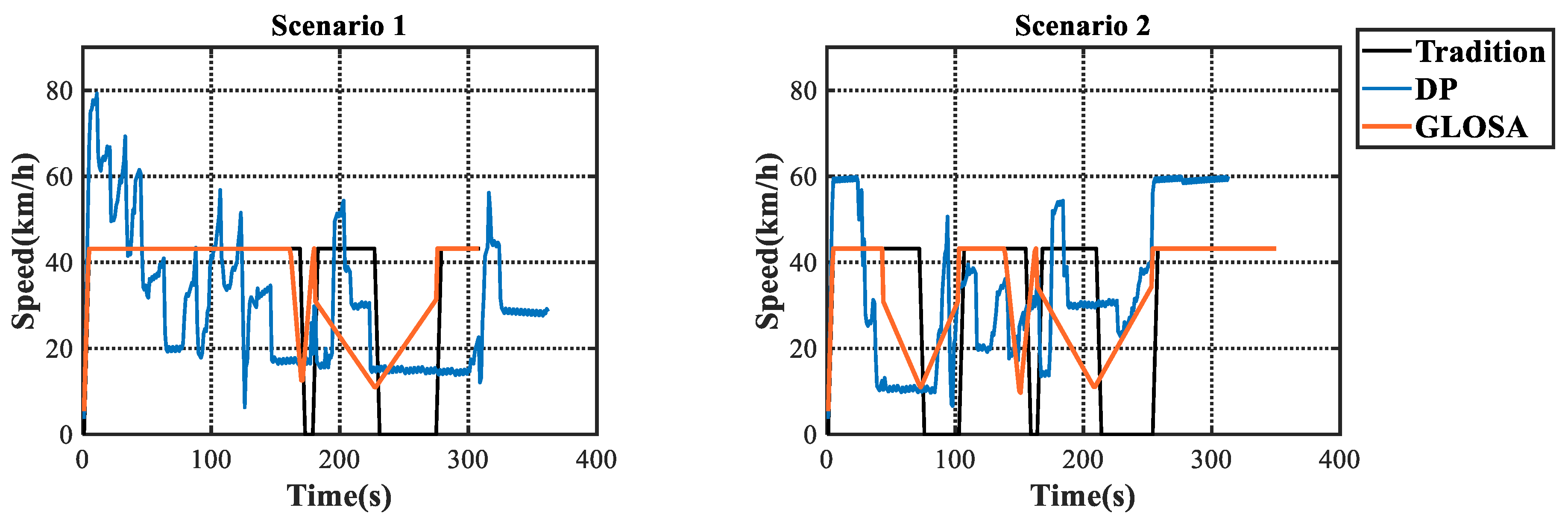
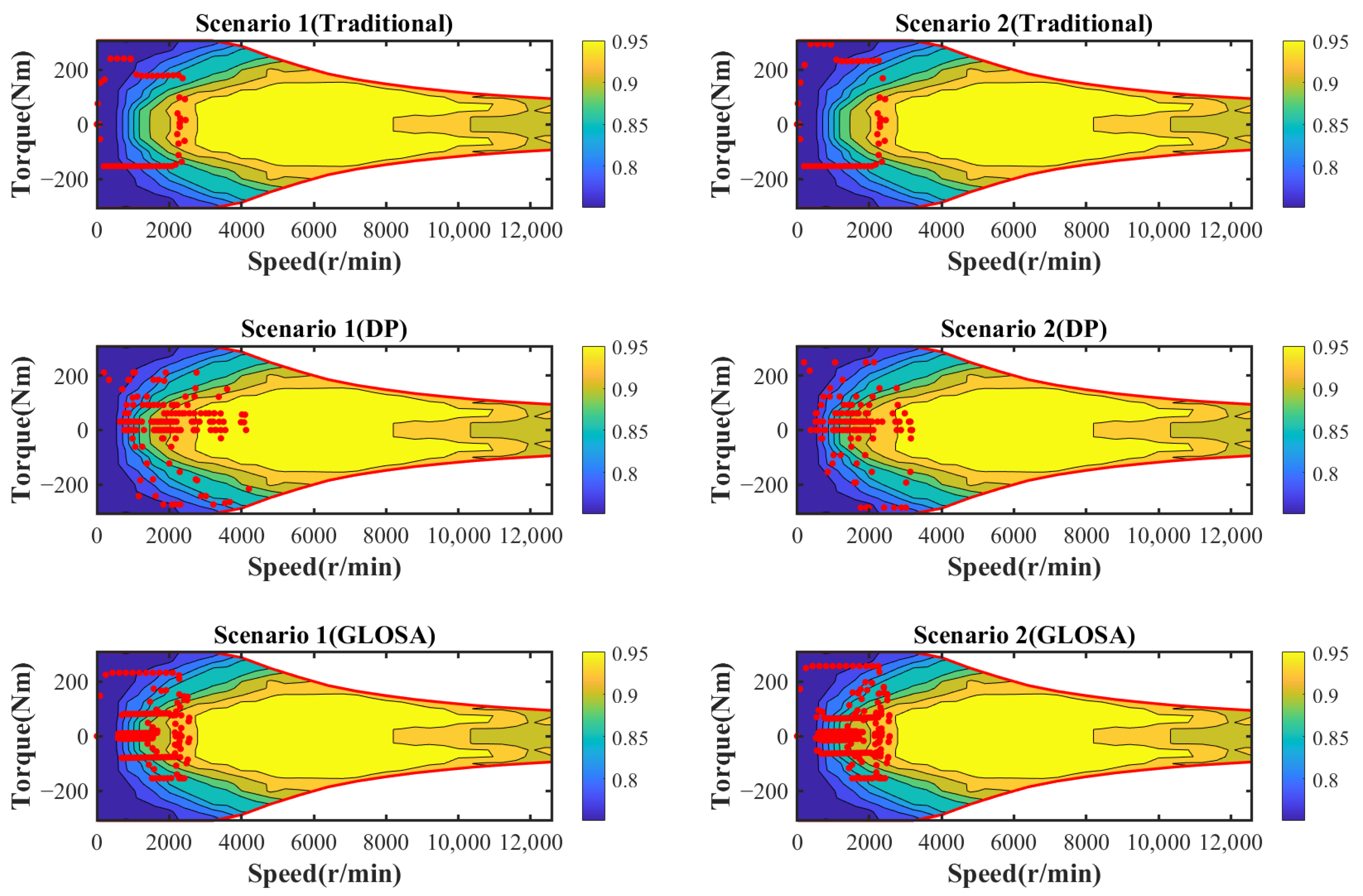
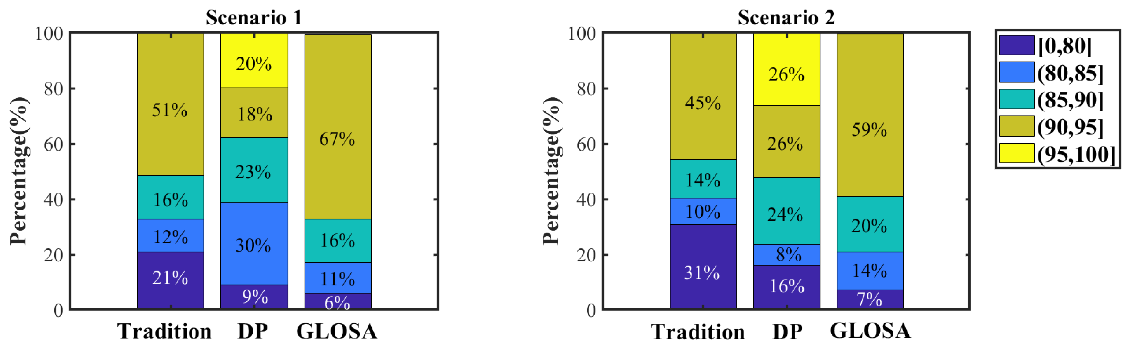
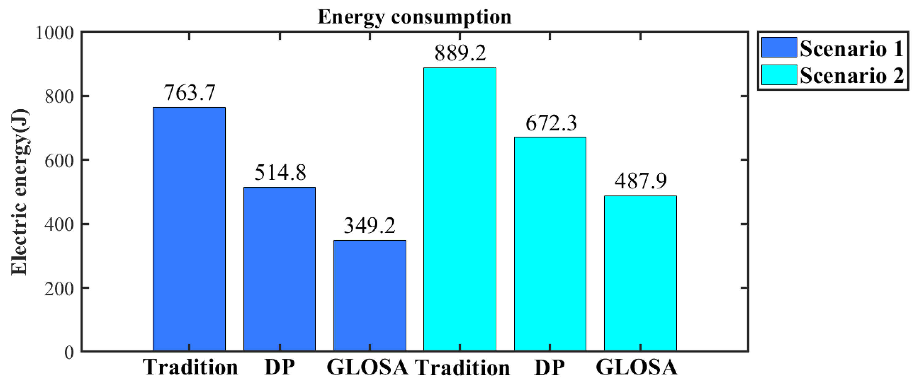
5.2. Simulation Analysis

Figure 7 shows the trend of vehicle speed with time in Scenarios 1 and 2 for all strategies. Figure 8 shows the time–space domain trajectories in Scenarios 1 and 2 for all strategies.

In Scenario 1, the fixed speed of the traditional strategy facilitates the vehicle to pass the first three traffic lights without stopping. However, at the last two traffic lights, two stops have to be made because it does not reach the intersection when the light is green. DP is a global energy management strategy, which can obtain traffic information in advance for the whole driving process to avoid parking. After passing the first two traffic lights at a higher speed, the vehicle adopts a lower average speed to cross the remaining three traffic lights. For a multiintersection passing task, the travel time of similar methods only depends on the passing scheme at the last intersection. If the vehicle arrives at the last intersection with a red light, it will start at the moment the traffic light turns green and achieve a shorter travel time. DP still maintains a relatively economical speed and requires more travel time. However, there was no serious impact on the overall task. In Scenario 2, the traditional strategy performs even worse due to there being three stops. The DP still does not make any stops. In order to pass the second traffic light without stopping, the DP undergoes a significant speed-up followed by a speed-down process. For the travel time, the DP reaches the end of the line first. Overall the time required for the two strategies displays no significant difference. For GLOSA, it utilizes traffic information to avoid stopping the vehicle. In general, it has the same trend as the traditional strategy. When crossing intersections, GLOSA can accelerate from a non-stopped state, so it has a time lead compared with the traditional strategy in different scenarios.

The economy is discussed in Figure 9, Figure 10 and Figure 11. Figure 9 shows the location of the motor operating point distribution for two scenarios, with different driving strategies. Figure 10 shows the results in the form of a bar chart displaying the number of operating points in different efficiency intervals. Figure 11 shows the total energy consumed by the driving task in different scenarios.

For each strategy, there is a large similarity in the location of the motor operating point distribution for the different scenarios. Since the traditional strategy has a fixed speed after vehicle starting, the distribution of operating points shows a clear border and does not reach more efficient area. The motor tends to achieve lower efficiency at a lower rotation speed. Therefore, the stopping and starting of the vehicle leads to the frequent switching of operating points between the inefficient and efficient areas. For DP, there is a tendency for operating points to be distributed around the contour and a larger number of operating points reach more efficient area. Compared with the traditional strategy, DP does not put the vehicle through a stop, and therefore achieves higher energy utilization efficiency. The distribution of the operating points of GLOSA is more concentrated overall. Still, none of the points reach the most efficient area.

Combining the analysis with Figure 10, for Scenario 1, the traditional solution does not have operating points within the efficiency of 95−100%. Instead, there are more operating points in the low efficiency area of 0–80% due to the presence of vehicle start–stop processes. Because of the simple acceleration process, there are fewer operating points that stay to 80–90%. For DP, since no vehicle start–stop process occurs, there are few operating points in the low efficiency area from 0−80%—only 9%. Additionally, 20% of the operating points have an efficiency of 95% or more. In Scenario 2, the same conclusion can be obtained. Scenario 1 is compared with Scenario 2 below. For the traditional strategy, the increase in the number of stops makes the operating point distribution of Scenario 2 worse. For DP, there are fewer operating points within the efficiency of 0–80% in scenario 1 and more operating points within the efficiency of 90–100% in Scenario 2. However, in Scenario 2 there are more operating points distributed in the 95–100% interval. In both scenarios, GLOSA performs similarly to the traditional strategy in the efficiency area of 80–90%. GLOSA outperforms the traditional strategy in both the 0−80% efficiency area and the 90–95% efficiency area.

The above analysis discusses only the number of operating points in each interval. In the following, the generated energy consumption will be analyzed in conjunction with Figure 11. In Scenario 1, the DP saves 54.27% of energy consumption compared with the traditional strategy and 32.17% of energy consumption compared with GLOSA. In Scenario 2, DP saves 45.13% and 27.43%. This shows that the signalized intersection passage process has a high energy saving potential. Comparing the different scenarios, the energy consumption of Scenario 1 will always be lower than that of Scenario 2 when the strategies are the same. This indicates that the initial phase of traffic lights in Scenario 1 is set more reasonably for the road.

Through simulation analysis, it can be seen that the constraints of the traffic light ensure that the vehicle passes on green and avoids stopping. DP greatly improves the economy of the vehicle under constraints.

6. Conclusions

In this paper, the optimal passing strategy for a multi-intersection passing task is solved by combining a traffic light model with a global-optimization-based energy management strategy. The traffic light model based on a vehicle–road cooperative system allows traffic lights to communicate with passing vehicles and impose constraints on vehicle speed to avoid unnecessary braking and acceleration at intersections. In order to eliminate the disturbance of different energy distribution from multiple power sources of vehicles under different speed profiles, this paper uses EV combined with a DP-based energy management strategy for the simulation. Combined with the constraints proposed by the traffic light model, DP adds a penalty to the constraints to ensure that the algorithm seeks a better control solution among more driving conditions. The results are validated for two scenarios with different initial phases and show that DP saves 54.27% and 45.13% of energy consumption in the two scenarios, respectively. Under the condition that the driving route is determined and the traffic light information is known, the speed planned by DP provides a reference for the driver and has an important energy saving value. The simulation results also show that the setting of the traffic light is also important for the vehicle. For the same driving tasks, the different phases of the traffic lights also affect the minimum energy consumption required for the vehicle passing.

In the future, the communication from the vehicle end to the road end will be used to design a dynamic adjustment scheme for timing and phase of traffic lights. In addition, the utilization of the optimal control solution provided by DP will be studied in depth.

References

1. Alturiman, A.; Alsabaan, M. Impact of Two-Way Communication of Traffic Light Signal-to-Vehicle on the Electric Vehicle State of Charge. IEEE Access 2019, 7, 8570–8581. [Google Scholar] [CrossRef]
2. Protschky, V.; Feld, S.; Walischmiller, M. Traffic Signal Adaptive Routing. In Proceedings of the 18th International Conference on Intelligent Transportation Systems, Las Palmas de Gran Canaria, Spain, 15–18 September 2015; pp. 450–456. [Google Scholar]
3. Mo, Y.H.; Zhang, P.L.; Chen, Z.J.; Ran, B. A Method of Vehicle-Infrastructure Cooperative Perception Based Vehicle State Information Fusion Using Improved Kalman Filter. Multimed. Tools. Appl. 2021, 18, 8199361. [Google Scholar] [CrossRef]
4. Wan, K.J.; Jeon, H.M.; Kim, S. Intelligent Wave/Dsrc Platform Technology for Efficient Data Transmission in Vehicle Communication. J. Korea Multimed. Soc. 2017, 20, 1519–1526. [Google Scholar]
5. Chen, S.Z.; Hu, J.L.; Shi, Y.; Zhao, L. LTE-V: A Td-Lte-Based V2x Solution for Future Vehicular Network. IEEE Internet. Things 2016, 3, 997–1005. [Google Scholar] [CrossRef]
6. Skondras, E.; Michalas, A.; Vergados, D.D. A Survey on Medium Access Control Schemes for 5G Vehicular Cloud Computing Systems. In Proceedings of the 2018 Global Information Infrastructure and Networking Symposium, Thessaloniki, Greece, 23–25 October 2018. [Google Scholar]
7. Li, J.; Dong, Y. A New Night Traffic Light Recognition Method. In Proceedings of the 2018 International Seminar on Computer Science and Engineering Technology, Shanghai, China, 17–18 December 2019. [Google Scholar]
8. Wang, J.G.; Zhou, L.B. Traffic Light Recognition with High Dynamic Range Imaging and Deep Learning. IEEE Trans. Intell. Transp. Syst. 2019, 20, 1341–1352. [Google Scholar] [CrossRef]
9. Kim, H.K.; Yoo, K.Y.; Park, J.H.; Jung, H.Y. Traffic Light Recognition Based on Binary Semantic Segmentation Network. Sensors 2019, 19, 1700. [Google Scholar] [CrossRef] [PubMed] [Green Version]
10. Zhang, P.; Yan, F.W.; Du, C.Q. A Comprehensive Analysis of Energy Management Strategies for Hybrid Electric Vehicles Based on Bibliometrics. Renew. Sustain. Energy Rev. 2015, 48, 88–104. [Google Scholar] [CrossRef]
11. Kim, M.; Jung, D.; Min, K. Hybrid Thermostat Strategy for Enhancing Fuel Economy of Series Hybrid Intracity Bus. IEEE Trans. Veh. Technol. 2014, 63, 3569–3579. [Google Scholar] [CrossRef]
12. Jeoung, H.; Lee, K.; Kim, N. Methodology for Finding Maximum Performance and Improvement Possibility of Rule-Based Control for Parallel Type-2 Hybrid Electric Vehicles. Energies 2019, 12, 1924. [Google Scholar] [CrossRef] [Green Version]
13. Liu, L.Z.; Zhang, B.Z.; Liang, H.Y. Global Optimal Control Strategy of PHEV Based on Dynamic Programming. In Proceedings of the 6th International Conference on Information Science and Control Engineering, Shanghai, China, 20–22 December 2019; pp. 758–762. [Google Scholar]
14. Hu, P.; Huang, C.; Lian, J. Efficient Dynamic Programming in Economical Cruise Control under Real-Time Traffic Situations. Trans. Inst. Meas. Control 2020, 42, 2044–2056. [Google Scholar] [CrossRef]
15. Rezaei, A.; Burl, J.B.; Zhou, B.; Rezaei, M. A New Real-Time Optimal Energy Management Strategy for Parallel Hybrid Electric Vehicles. IEEE Trans. Contr. Syst. Technol. 2019, 27, 830–837. [Google Scholar] [CrossRef]
16. Keller, M.; Schmitt, L.; Abel, D. Nonlinear Hierarchical Model Predictive Control for the Energy Management of a Hybrid Electric Vehicle. In Proceedings of the 27th Mediterranean Conference on Control and Automation, Akko, Israel, 1–4 July 2019; pp. 451–457. [Google Scholar]
17. Altan, O.D.; Wu, G.; Barth, M.J.; Boriboonsomsin, K.; Stark, J.A. Glidepath: Eco-Friendly Automated Approach and Departure at Signalized Intersections. IEEE Trans. Intell. Veh. 2017, 2, 266–277. [Google Scholar] [CrossRef]
18. Wang, Z.; Wu, G.; Barth, M.J. Cooperative Eco-Driving at Signalized Intersections in a Partially Connected and Automated Vehicle Environment. IEEE Trans. Intell. Transp. 2019, 21, 2029–2038. [Google Scholar] [CrossRef] [Green Version]
19. Yu, S.W.; Fu, R.; Guo, Y.S.; Xin, Q.; Shi, Z.K. Consensus and Optimal Speed Advisory Model for Mixed Traffic at an Isolated Signalized Intersection. Phys. A 2019, 531, 1–22. [Google Scholar] [CrossRef]
20. Suzuki, H.; Marumo, Y. A New Approach to Green Light Optimal Speed Advisory (GLOSA) Systems for High-Density Traffic Flow. In Proceeding of the 21st IEEE International Conference on Intelligent Transportation Systems, Maui, HI, USA, 4–7 November 2018; pp. 362–367. [Google Scholar]
21. Luo, Z.; Li, Y.; Zhang, X.; Wang, K. Vector control implementation in field programmable gate array for 200 kHz GaN-based motor drive systems. J. Eng. 2018, 13, 650–653. [Google Scholar] [CrossRef]
22. Park, C.H.; Eui, Y.G. Development and Performance of BMS Modules for Urban Electric Car Using Life Prediction Method. Trans. KSAE 2013, 21, 147–154. [Google Scholar]
23. Kang, G. A Law and Policy Study on Tuning of Automotive Electronic Control Units(ECU). Han Yang Law Rev. 2020, 3, 145–168. [Google Scholar] [CrossRef]
24. Blekhman, I.; Kremer, E. Vertical-longitudinal dynamics of vehicle on road with unevenness. In Proceedings of the 10th International Conference on Structural Dynamics, Rome, Italy, 10–13 September 2017; pp. 3278–3283. [Google Scholar]
25. Liu, Z.X.; Wang, Z.; Bai, X.P.; Gao, L. Linearized Longitudinal Dynamic Model for Tractor Cruise Control System. In Proceedings of the 10th International Conference on Computer Modelling and Simulation, Sydney, Australia, 8–10 January 2018; pp. 221–227. [Google Scholar]
26. Huang, K.F.; Wang, Y.; Feng, J.Q. Research on Equivalent Circuit Model of Lithium-ion Battery for Electric Vehicles. In Proceedings of the 3rd World Conference on Mechanical Engineering and Intelligent Manufacturing, Shanghai, China, 4–6 December 2020; pp. 492–496. [Google Scholar]
27. Kim, T.; Qiao, W. A Hybrid Battery Model Capable of Capturing Dynamic Circuit Characteristics and Nonlinear Capacity Effects. IEEE Trans. Energy Conver. 2011, 26, 1172–1180. [Google Scholar] [CrossRef] [Green Version]
28. Ndashimye, E.; Ray, S.K.; Sarkar, N.I.; Gutierrez, J.A. Vehicle-to-Infrastructure Communication over Multi-Tier Heterogeneous Networks: A Survey. Comput. Netw. 2017, 112, 144–166. [Google Scholar] [CrossRef]
29. Topaloglu, H.; Kunnumkal, S. Approximate dynamic programming methods for an inventory allocation problem under uncertainty. Nav. Res. Logist. 2006, 8, 822–841. [Google Scholar] [CrossRef] [Green Version]
30. Fan, J.J.; Guo, J.Y.; Wang, L.; Zhu, J.P.; Zhang, X.F. Dynamic Programming Algorithm for Hybrid Powertrain Power Allocation. In Proceedings of the 38th Chinese Control Conference, Guangzhou, China, 27–30 July 2019; pp. 6674–6679. [Google Scholar]
Figure 1. The schematic of the EV configuration.
Electronics 10 02295 g001
Figure 2. Motor efficiency contour map.
Electronics 10 02295 g002
Figure 3. Cooperative vehicle infrastructure system framework.
Electronics 10 02295 g003
Figure 4. Illustration of discretization constraints.
Electronics 10 02295 g004
Figure 5. The color of the next target traffic light is red.
Electronics 10 02295 g005
Figure 6. The color of the next target traffic light is green.
Electronics 10 02295 g006
Figure 7. Time–speed curves of different scenarios.
Electronics 10 02295 g007
Figure 8. Time–space domain trajectories of different scenarios.
Electronics 10 02295 g008
Figure 9. Motor operating point distribution diagram.
Electronics 10 02295 g009
Figure 10. Percentage of the number of operating points in each efficiency area.
Electronics 10 02295 g010
Figure 11. Energy consumption for different scenarios and strategies.
Electronics 10 02295 g011