
Improved Model Predictive Control for Asymmetric T-Type NPC 3-Level Inverter


Abstract
:1. Introduction
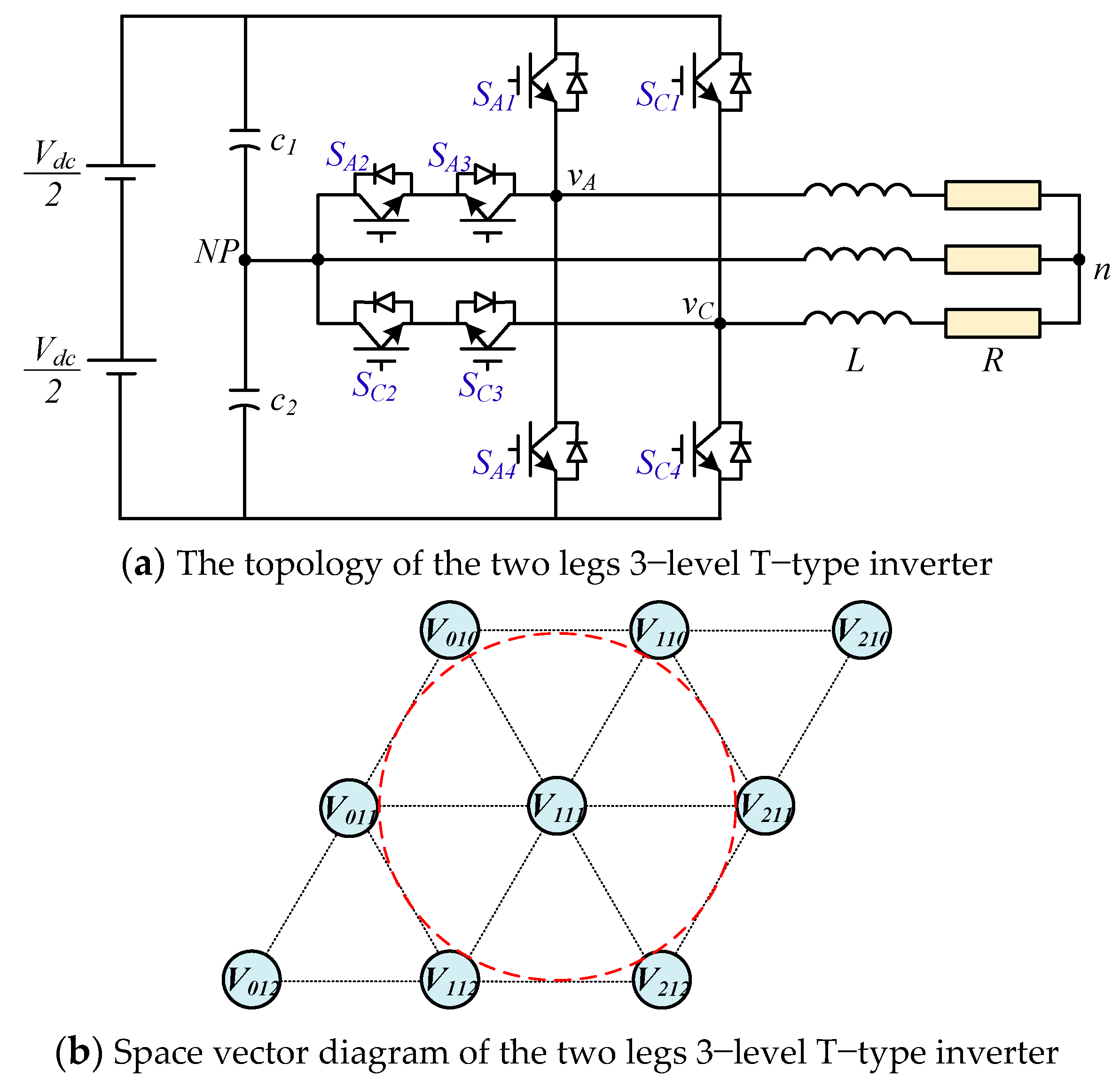
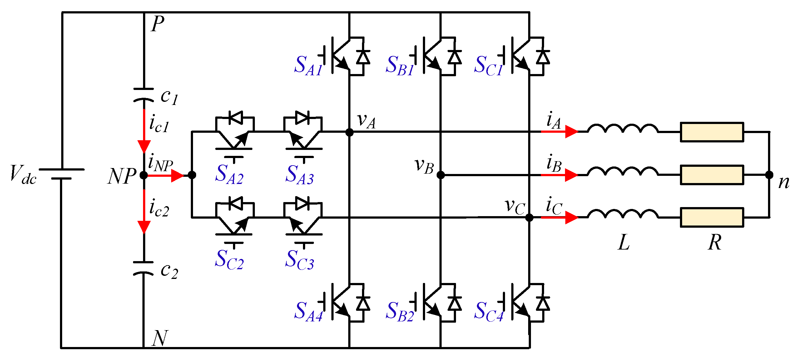
2. Mathematical Model of Asymmetric 3-Level T-Type NPC Inverter
3. Proposed MPC for Asymmetric T-Type NPC 3-Level Inverter
3.1. Current Tracking Control
3.2. DC-Link Capacitor Voltage Balancing
3.3. Global Cost Function
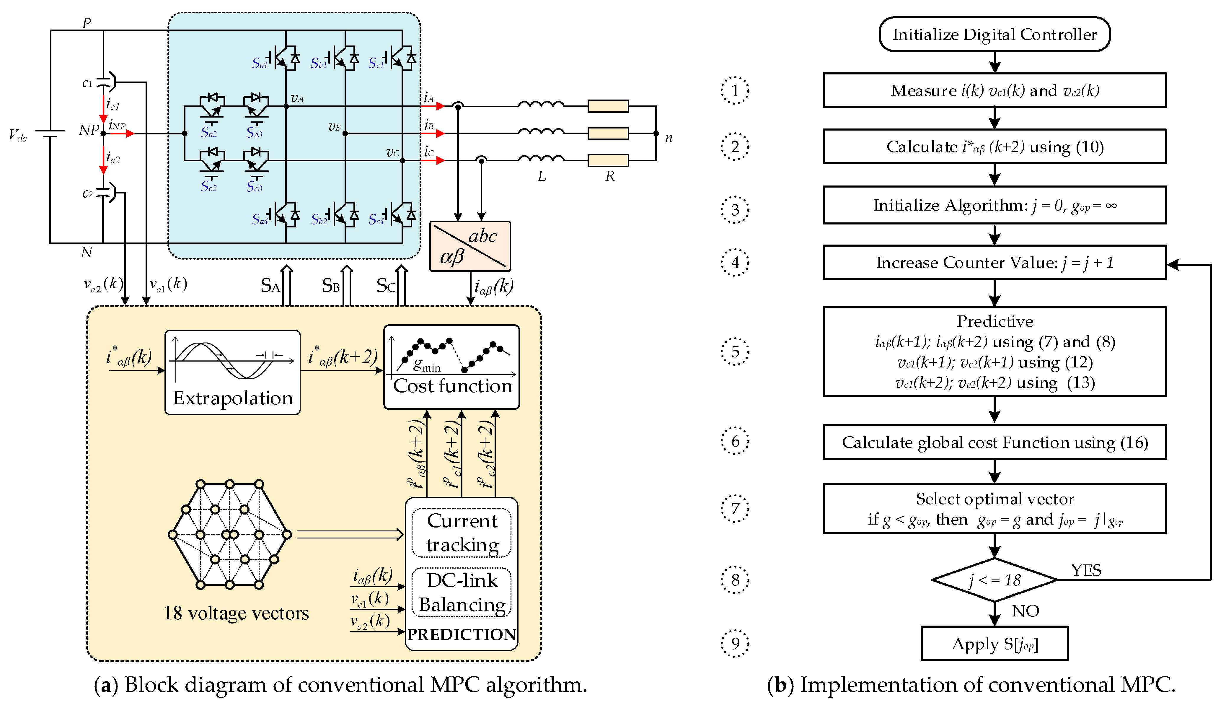
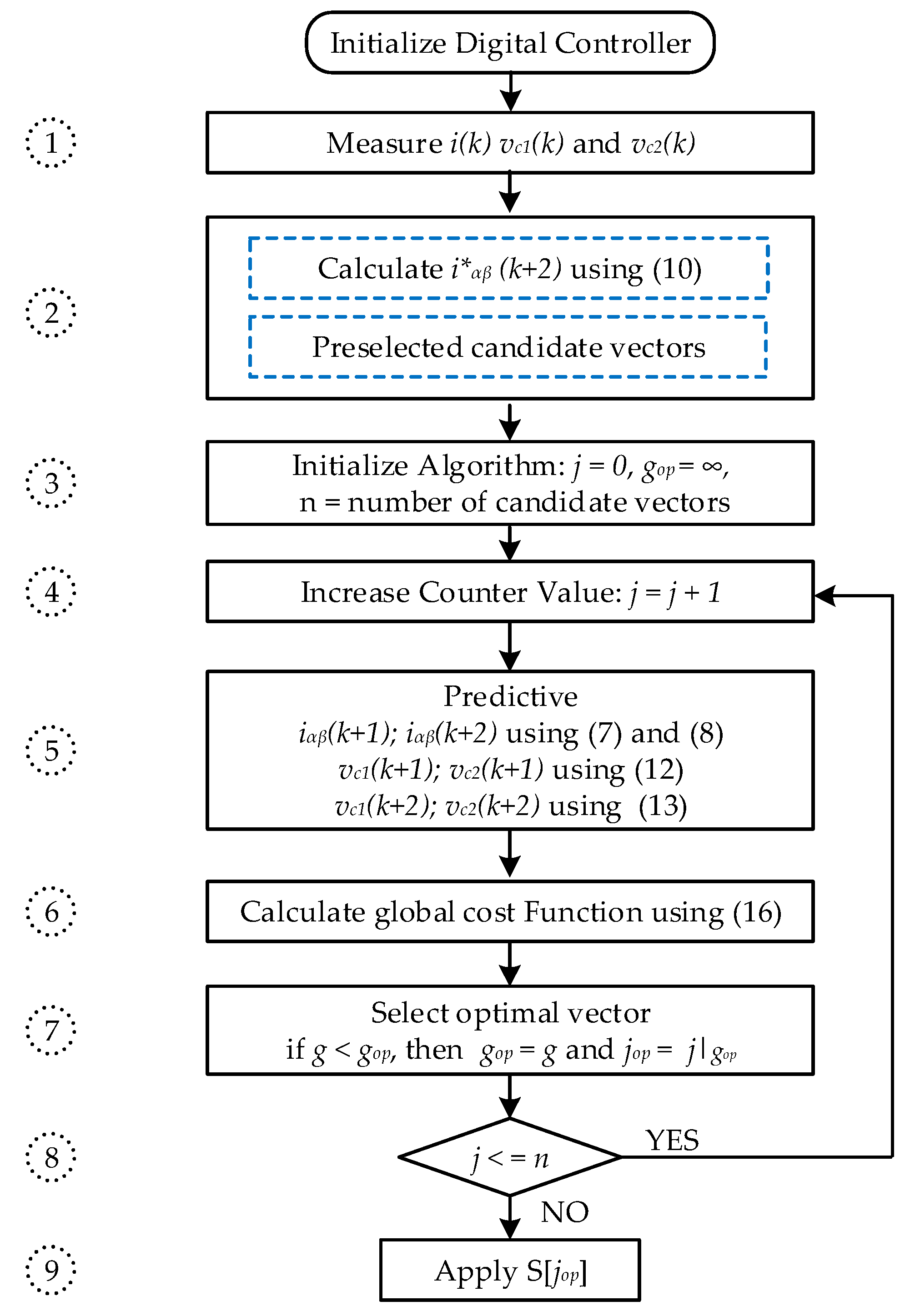
- ➀
- Measure current, capacitor voltages from sensor feedback signals;
- ➁
- The reference current at the time is calculated by extrapolation;
- ➂
- Initialize the initial values;
- ➃
- Enter the loop, where the counter increases j value in steps;
- ➄
- The output current and DC capacitor voltages are predicted to time corresponding to each candidate vector;
- ➅
- Calculate the global cost function;
- ➆
- During any iteration, if , the minimum of value is stored as an optimal value and the corresponding position is stored as ;
- ➇
- Check the loop condition, if 18 is true then return to execute the tasks from step 4, if false, exit the loop and continue to step 9;
- ➈
- Apply the switching states based on the value.
3.4. Improved Algorithm
4. Simulation and Experimental Results
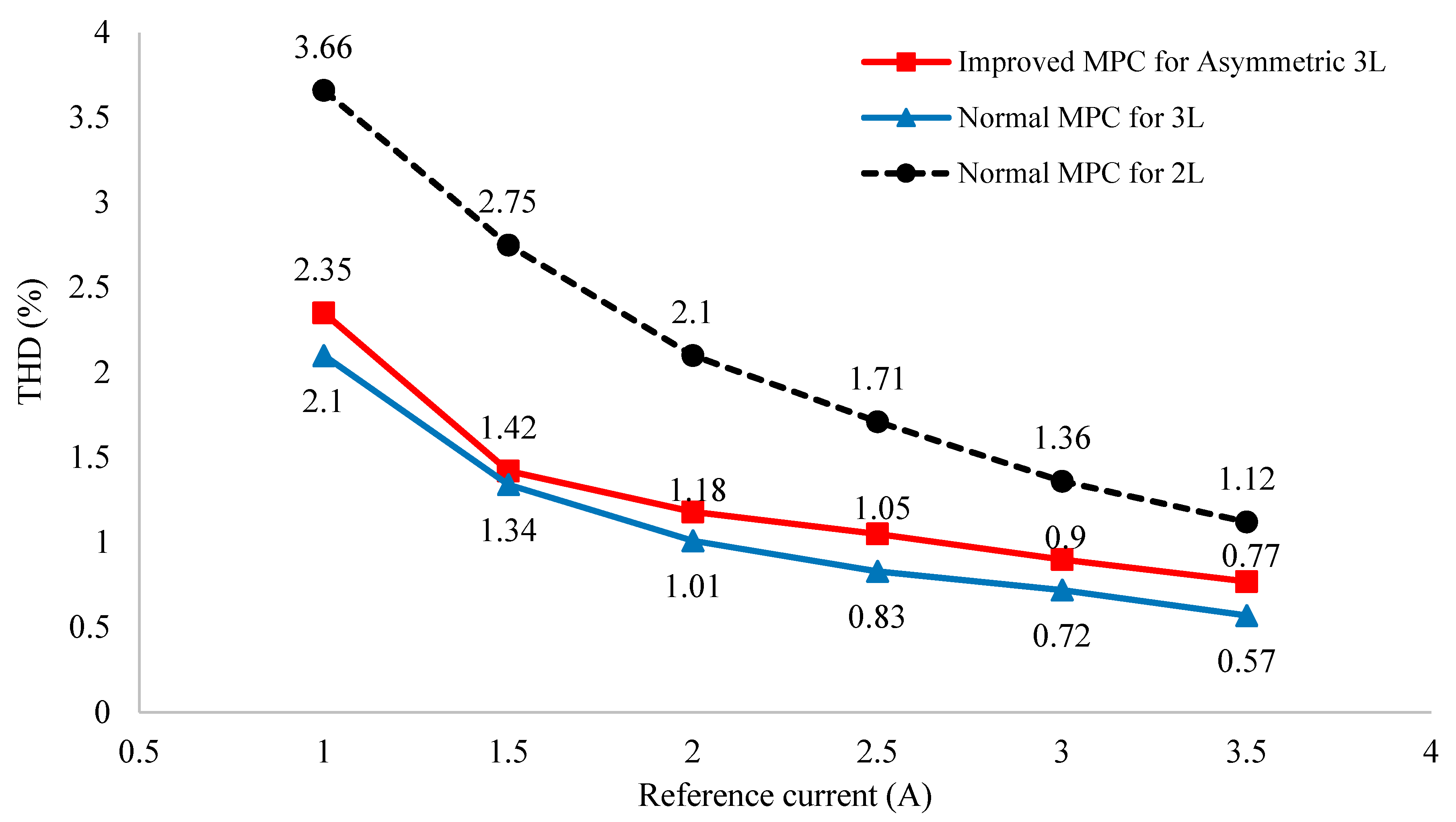
4.1. Simulation Results
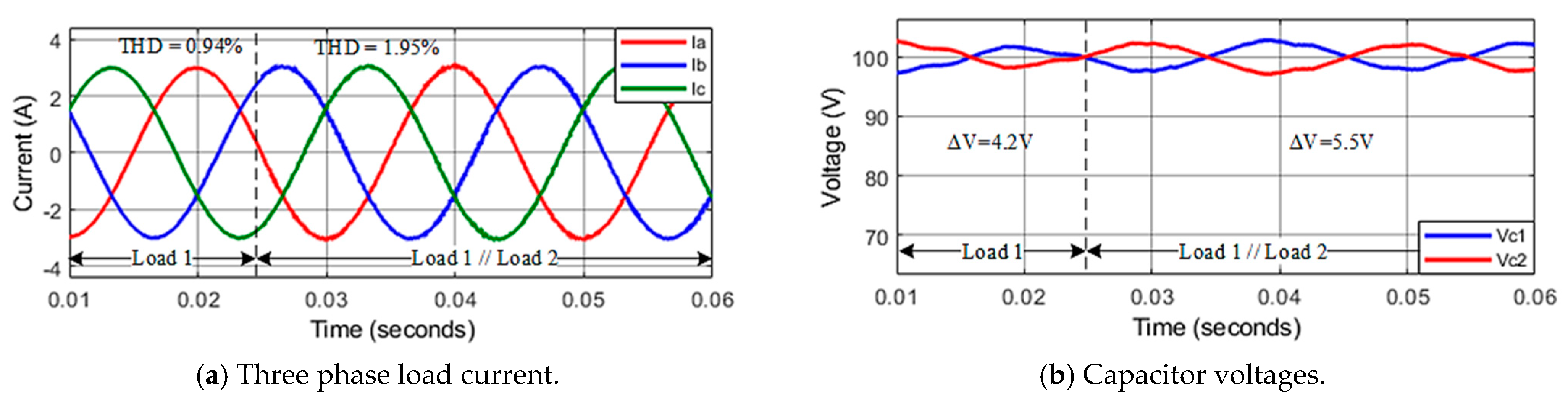
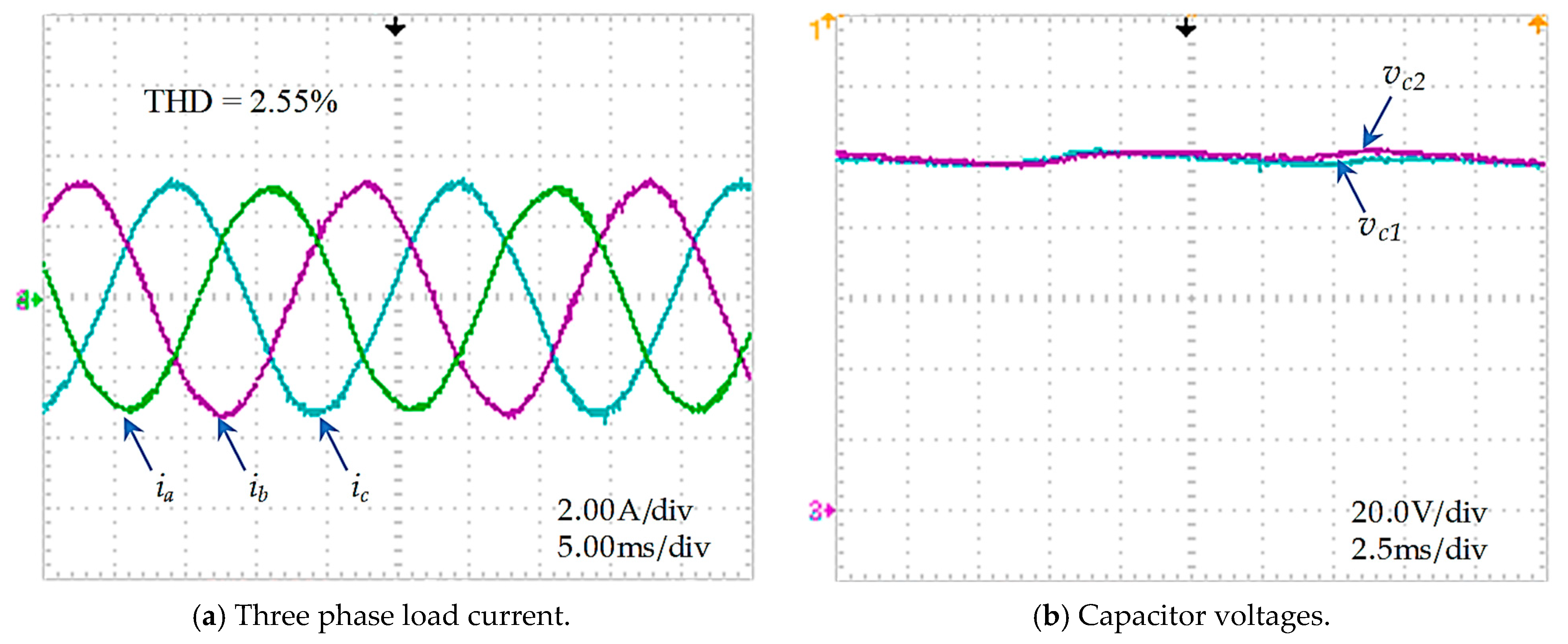
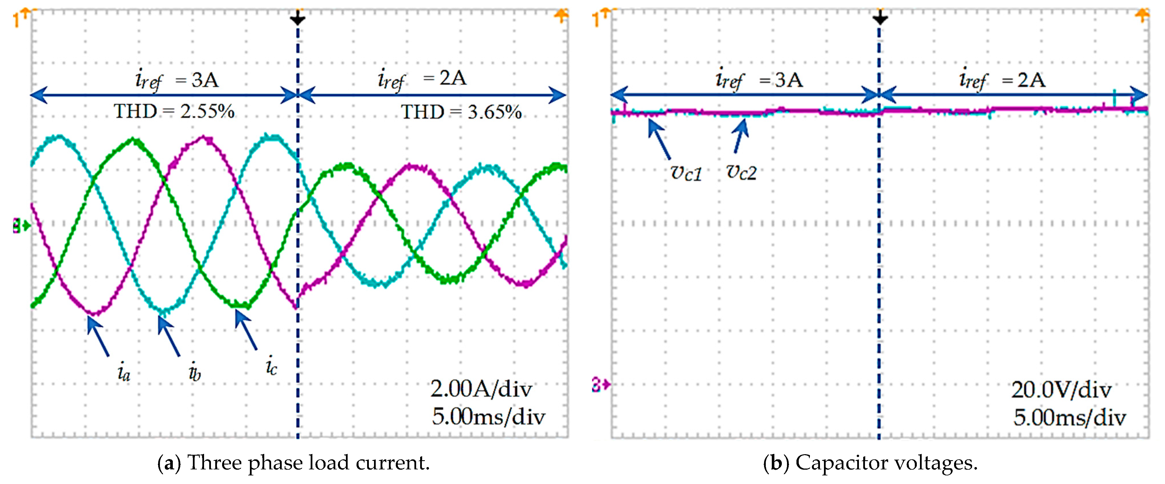
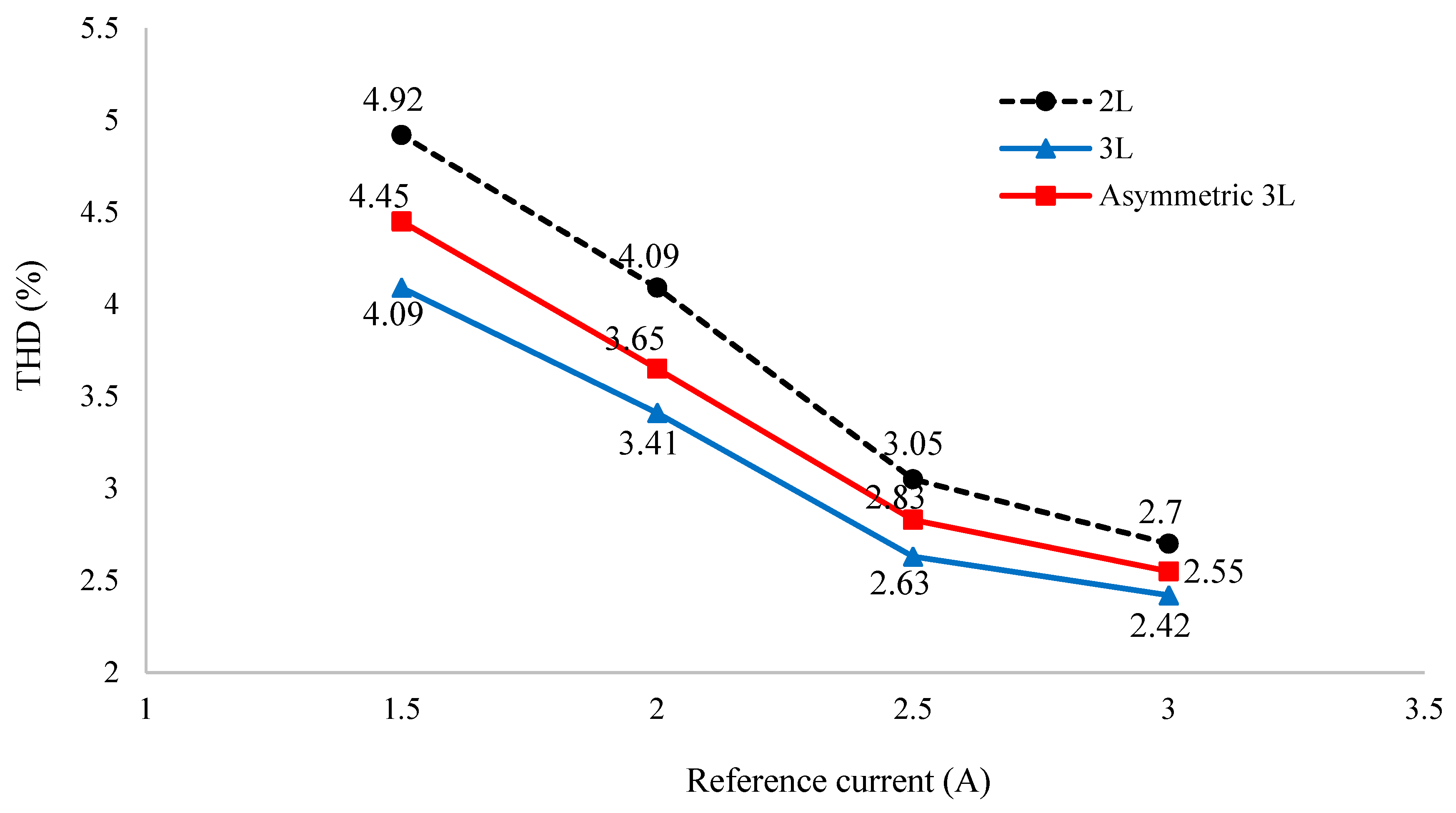
4.2. Experimental Results
5. Conclusions
Author Contributions
Funding
Conflicts of Interest
References
- Davoodnezhad, R.; Holmes, D.G.; McGrath, B.P. A Novel Three-Level Hysteresis Current Regulation Strategy for Three-Phase Three-Level Inverters. IEEE Trans. Power Electron. 2013, 29, 6100–6109. [Google Scholar] [CrossRef]
- Mukherjee, S.; Giri, S.K.; Kundu, S.; Banerjee, S. A Generalized Discontinuous PWM Scheme for Three-Level NPC Traction Inverter With Minimum Switching Loss for Electric Vehicles. IEEE Trans. Ind. Appl. 2019, 55, 516–528. [Google Scholar] [CrossRef]
- Singh, R.; Bansal, R.C.; Singh, A.R.; Naidoo, R. Multi-Objective Optimization of Hybrid Renewable Energy System Using Reformed Electric System Cascade Analysis for Islanding and Grid Connected Modes of Operation. IEEE Access 2018, 6, 47332–47354. [Google Scholar] [CrossRef]
- Choudhury, A.; Pillay, P.; Williamson, S.S. Comparative Analysis Between Two-Level and Three-Level DC/AC Electric Vehicle Traction Inverters Using a Novel DC-Link Voltage Balancing Algorithm. IEEE J. Emerg. Sel. Top. Power Electron. 2014, 2, 529–540. [Google Scholar] [CrossRef]
- Annoukoubi, M.; Essadki, A.; Laghridat, H.; Nasser, T. Comparative study between the performances of a three-level and two-level converter for a Wind Energy Conversion System. In Proceedings of the 2019 International Conference on Wireless Technologies, Embedded and Intelligent Systems (WITS), Fez, Morocco, 3–4 April 2019; IEEE: Manhattan, NY, USA, 2019; pp. 1–6. [Google Scholar]
- Teichmann, R.; Bernet, S. A Comparison of Three-Level Converters Versus Two-Level Converters for Low-Voltage Drives, Traction, and Utility Applications. IEEE Trans. Ind. Appl. 2005, 41, 855–865. [Google Scholar] [CrossRef]
- Choi, U.M.; Blaabjerg, F.; Lee, K.-B. Reliability Improvement of a T-Type Three-Level Inverter With Fault-Tolerant Control Strategy. IEEE Trans. Power Electron. 2015, 30, 2660–2673. [Google Scholar] [CrossRef]
- Alemi, P.; Jeung, Y.C.; Lee, D.C. DC-Link Capacitance Minimization in T-Type Three-Level AC/DC/AC PWM Converters. IEEE Trans. Ind. Electron. 2015, 62, 1382–1391. [Google Scholar] [CrossRef]
- Schweizer, M.; Friedli, T.; Kolar, J.W. Comparative Evaluation of Advanced Three Phase Three-Level Inverter/Converter Topologies against Two-Level Systems. IEEE Trans. Ind. Electron. 2013, 60, 5515–5527. [Google Scholar] [CrossRef]
- Alemi, P.; Lee, D.C. Comparative Analysis of Power Losses for Three-Level T-Type and NPC PWM Inverters. Trans. Korean Inst. Power Electron. 2014, 19, 173–183. [Google Scholar] [CrossRef] [Green Version]
- Patsakis, G.; Karamanakos, P.; Stolze, P.; Manias, S.; Kennel, R.; Mouton, H.D.T. Variable switching point predictive torque control for the four-switch three-phase inverter. In Proceedings of the 2013 IEEE International Symposium on Sensorless Control for Electrical Drives and Predictive Control of Electrical Drives and Power Electronics (SLED/PRECEDE), Munich, Germany, 17–19 October 2013; IEEE: Manhattan, NY, USA, 2013; pp. 1–8. [Google Scholar]
- Sefa, I.; Komurcugil, H.; Demirbas, S.; Altin, N.; Ozdemir, S. Three-phase three-level inverter with reduced number of switches for stand-alone PV systems. In Proceedings of the 2017 IEEE 6th International Conference on Renewable Energy Research and Applications (ICRERA), San Diego, CA, USA, 5–8 November 2017; IEEE: Manhattan, NY, USA, 2017; pp. 1119–1124. [Google Scholar]
- Tarek, G.; Badii, B.; Ahmed, M. DTC of reconfigured three level inverter fed IM drives following a leg failure. COMPEL Int. J. Comput. Math. Electr. 2016, 35, 764–781. [Google Scholar]
- Ozdemir, S.; Altin, N.; Komurcugil, H.; Sefa, I. Sliding Mode Control of Three-Phase Three-Level Two-Leg NPC Inverter with LCL Filter for Distributed Generation Systems. In Proceedings of the IECON 2018—44th Annual Conference of the IEEE Industrial Electronics Society, Washington, DC, USA, 21–23 October 2018; IEEE: Manhattan, NY, USA, 2018; pp. 3895–3900. [Google Scholar]
- Heydari, M.; Fatemi, A.; Varjani, A.Y. A Reduced Switch Count Three-Phase AC/AC Converter With Six Power Switches: Modeling, Analysis, and Control. IEEE J. Emerg. Sel. Top. Power Electron. 2017, 5, 1720–1738. [Google Scholar] [CrossRef]
- Vidhya, V.; Balamurugan, C.R.; Natarajan, S.P. Investigation on symmetrical three phase hybrid cascaded multilevel inverter with reduced number of switches. In Proceedings of the DST Sponsored International Conference on Power and Energy System ICPES’12, Las Vegas, NV, USA, 12–14 November 2012. [Google Scholar]
- Altin, N.; Sefa, I.; Komurcugil, H.; Ozdemir, S. Three-phase three-level T-type grid-connected inverter with reduced number of switches. In Proceedings of the 2018 6th International Istanbul Smart Grids and Cities Congress and Fair (ICSG), Istanbul, Turkey, 25–26 April 2018; Institute of Electrical and Electronics Engineers (IEEE): Manhattan, NY, USA, 2018; pp. 58–62. [Google Scholar]
- Nachiappan, A.; Sundararajan, K.; Malarselvam, V. Current controlled voltage source inverter using Hysteresis controller and PI controller. In Proceedings of the 2012 International Conference on Power, Signals, Controls and Computation, Thrissur, Kerala, 3–6 January 2012; IEEE: Manhattan, NY, USA, 2012; pp. 1–6. [Google Scholar]
- Kwon, T.-S.; Sul, S.-K. Novel Antiwindup of a Current Regulator of a Surface-Mounted Permanent-Magnet Motor for Flux-Weakening Control. IEEE Trans. Ind. Appl. 2006, 42, 1293–1300. [Google Scholar] [CrossRef]
- Kawabata, T.; Miyashita, T.; Yamamoto, Y. Dead beat control of three phase PWM inverter. IEEE Trans. Power Electron. 1990, 5, 21–28. [Google Scholar] [CrossRef]
- Kukrer, O. Discrete-time current control of voltage-fed three-phase PWM inverters. IEEE Trans. Power Electron. 1996, 11, 260–269. [Google Scholar] [CrossRef]
- Lee, D.-C.; Sul, S.-K.; Park, M.-H. Comparison of AC current regulators for IGBT inverter. In Proceedings of the Conference Record of the Power Conversion Conference, Yokohama, Japan, 9–12 April 1993; Institute of Electrical and Electronics Engineers (IEEE): Manhattan, NY, USA, 2002; pp. 206–212. [Google Scholar]
- Ngo, V.-Q.-B.; Nguyen, M.-K.; Tran, T.-T.; Lim, Y.-C.; Choi, J.-H. A Simplified Model Predictive Control for T-Type Inverter with Output LC Filter. Energies 2019, 12, 31. [Google Scholar] [CrossRef] [Green Version]
- Cortes, P.; Rodriguez, J.; Silva, C.; Flores, A. Delay Compensation in Model Predictive Current Control of a Three-Phase Inverter. IEEE Trans. Ind. Electron. 2012, 59, 1323–1325. [Google Scholar] [CrossRef]
- Vatani, M.; Hovd, M.; Molinas, M. Finite Control Set Model Predictive Control of a shunt active power filter. In Proceedings of the 2013 Twenty-Eighth Annual IEEE Applied Power Electronics Conference and Exposition (APEC), Long Beach, CA, USA, 17–21 March 2013; Institute of Electrical and Electronics Engineers (IEEE): Manhattan, NY, USA, 2013; pp. 2156–2161. [Google Scholar]
- Xue, C.; Zhou, D.; Li, Y. Finite-Control-Set Model Predictive Control for Three-Level NPC Inverter-Fed PMSM Drives With LC Filter. IEEE Trans. Ind. Electron. 2021, 68, 11980–11991. [Google Scholar] [CrossRef]
- Cortes, P.; Kazmierkowski, M.P.; Kennel, R.M.; Quevedo, D.E.; Rodriguez, J. Predictive Control in Power Electronics and Drives. IEEE Trans. Ind. Electron. 2008, 55, 4312–4324. [Google Scholar] [CrossRef]
- Aurtenechea, S.; Rodríguez, M.A.; Oyarbide, E.; Torrealday, J.R. Predictive control strategy for dc/ac converters based on direct power control. IEEE Trans. Ind. Electron. 2007, 54, 1261–1271. [Google Scholar]
- Aurtenechea, S.; Rodriguez, M.A.; Oyarbide, E.; Torrealday, J.R. Predictive direct power control—A new control strate-gy for DC/AC converters. In Proceedings of the IECON 2006-32nd Annual Conference on IEEE Industrial Electronics, Paris, France, 7–10 November 2006; pp. 1661–1666. [Google Scholar]
- Zhang, Z.; Fang, H.; Gao, F.; Rodriguez, J.; Kennel, R. Multiple-Vector Model Predictive Power Control for Grid-Tied Wind Turbine System With Enhanced Steady-State Control Performance. IEEE Trans. Ind. Electron. 2017, 64, 6287–6298. [Google Scholar] [CrossRef]
- Yaramasu, V.; Wu, B. Model Predictive Control of Wind Energy Conversion Systems; Wiley-IEEE Press: New York, NY, USA, 2017; ISBN 978-1-118-98858-9. [Google Scholar]
- Calle-Prado, A.; Alepuz, S.; Bordonau, J.; Nicolas-Apruzzese, J.; Cortes, P.; Rodriguez, J. Model Predictive Current Control of Grid-Connected Neutral-Point-Clamped Converters to Meet Low-Voltage Ride-Through Requirements. IEEE Trans. Ind. Electron. 2015, 62, 1503–1514. [Google Scholar] [CrossRef] [Green Version]
- Bruckner, T.; Bernet, S.; Guldner, H. The Active NPC Converter and Its Loss-Balancing Control. IEEE Trans. Ind. Electron. 2005, 52, 855–868. [Google Scholar] [CrossRef]


| For Phasewith | For Phase B | ||||||||
|---|---|---|---|---|---|---|---|---|---|
| Switching State | Device State | Output Voltage | Switching State | Device State | Output Voltage | ||||
| 2 | 1 | 1 | 0 | 0 | 2 | 1 | 0 | ||
| 1 | 0 | 1 | 1 | 0 | - | - | - | - | |
| 0 | 0 | 0 | 1 | 1 | 0 | 0 | 0 | 1 | 0 |
| Type | Switching State | Output Voltage | Voltage Vector | ||
|---|---|---|---|---|---|
| SASBSC | |||||
| Zero voltage vector | 000 | 0 | 0 | 0 | |
| 222 | |||||
| Small voltage vector | 100 | 0 | 0 | ||
| 221 | |||||
| 121 | |||||
| 122 | |||||
| 001 | 0 | 0 | |||
| 101 | 0 | ||||
| Medium voltage vector | 120 | 0 | |||
| 021 | 0 | ||||
| 102 | 0 | ||||
| 201 | 0 | ||||
| Large voltage vector | 200 | 0 | 0 | ||
| 220 | 0 | ||||
| 020 | 0 | 0 | |||
| 022 | 0 | ||||
| 002 | 0 | 0 | |||
| 202 | 0 | ||||
| Characteristic | 2-Level | 3-Level | Asymmetric 3-Level |
|---|---|---|---|
| Structure | +Symmetric +Using 6 IGBTs | +Symmetric +Using 12 IGBTs | +Asymmetric +Using 10 IGBTs |
| Switching states | 8 | 27 | 18 |
| Different voltage vectors | 7 | 19 | 17 |
| Line voltage levels |
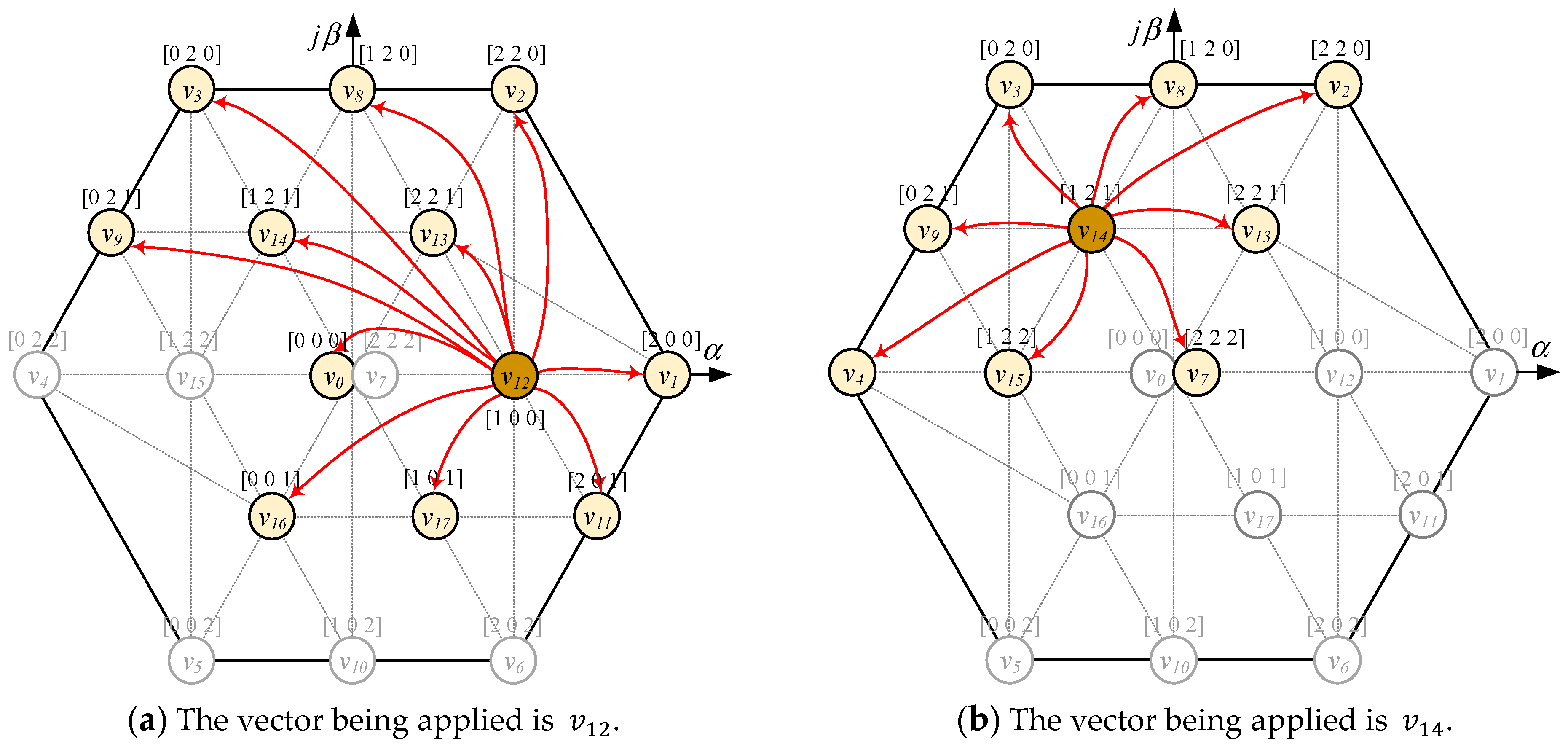
| Vector | The Candidate Voltage Vectors | Vector | The Candidate Voltage Vectors |
|---|---|---|---|
| v0 | v0, v3, v8, v9, v12, v14, v16, v17 | v9 | v0, v3, v4, v5, v8, v9, v10, v12, v13, v14, v15, v17 |
| v1 | v1, v8, v10, v11, v12, v13, v14, v17 | v10 | v4, v5, v6, v7, v9, v10, v11, v13, v14, v15, v16, v17 |
| v2 | v2, v8, v11, v12, v13, v14, v15, v17 | v11 | v1, v2, v6, v7, v8, v10, v11, v12, v13, v14, v15, v17 |
| v3 | v0, v3, v8, v9, v12, v14, v16, v17 | v12 | v0, v1, v2, v3, v8, v9, v11, v12, v13, v14, v16, v17 |
| v4 | v4, v5, v9, v10, v14, v15, v16, v17 | v13 | v1, v2, v7, v8, v10, v11, v12, v13, v14, v15, v16, v17 |
| v5 | v4, v5, v9, v10, v14, v15, v16, v17 | v14 | v2, v3, v4, v7, v8, v9, v13, v14, v15 |
| v6 | v6, v7, v10, v11, v13, v14, v15, v17 | v15 | v4, v5, v6, v7, v9, v10, v11, v13, v14, v15, v16, v17 |
| v7 | v6, v7, v10, v11, v13, v14, v15, v17 | v16 | v0, v3, v4, v5, v8, v9, v10, v12, v14, v15, v16, v17 |
| v8 | v0, v1, v2, v3, v8, v9, v11, v12, v13, v14, v16, v17 | v17 | v0, v1, v5, v6, v10, v11, v12, v16, v17 |
| Description | Variable | Value |
|---|---|---|
| DC voltage | 200 V | |
| Load 1 | , | 25 Ω, 50 mH |
| Load 2 | , | 25 Ω, 50 mH |
| DC-link capacitor | 1200 μF | |
| Sampling frequency | 20 kHz | |
| Frequency | 50 Hz | |
| Weighting factor | 0.005 |
Publisher’s Note: MDPI stays neutral with regard to jurisdictional claims in published maps and institutional affiliations. |
© 2021 by the authors. Licensee MDPI, Basel, Switzerland. This article is an open access article distributed under the terms and conditions of the Creative Commons Attribution (CC BY) license (https://creativecommons.org/licenses/by/4.0/).
Share and Cite
Doan, N.X.; Nguyen, N.V. Improved Model Predictive Control for Asymmetric T-Type NPC 3-Level Inverter. Electronics 2021, 10, 2244. https://doi.org/10.3390/electronics10182244
Doan NX, Nguyen NV. Improved Model Predictive Control for Asymmetric T-Type NPC 3-Level Inverter. Electronics. 2021; 10(18):2244. https://doi.org/10.3390/electronics10182244
Chicago/Turabian StyleDoan, Nam Xuan, and Nho Van Nguyen. 2021. "Improved Model Predictive Control for Asymmetric T-Type NPC 3-Level Inverter" Electronics 10, no. 18: 2244. https://doi.org/10.3390/electronics10182244
APA StyleDoan, N. X., & Nguyen, N. V. (2021). Improved Model Predictive Control for Asymmetric T-Type NPC 3-Level Inverter. Electronics, 10(18), 2244. https://doi.org/10.3390/electronics10182244