Identifying Communication Topologies on Twitter

Abstract

Social networks are known for their decentralization and democracy. Each individual has a chance to participate and influence any discussion. Even with all the freedom, people’s behavior falls under patterns that are observed in numerous situations. In this paper, we propose a methodology that defines and searches for common communication patterns in topical networks on Twitter. We analyze clusters according to four traits: number of nodes the cluster has, their degree and betweenness centrality values, number of node types, and whether the cluster is open or closed. We find that cluster structures can be defined as (a) fixed, meaning that they are repeated across datasets/topics following uniform rules, or (b) variable if they follow an underlying rule regardless of their size. This approach allows us to classify 90% of all conversation clusters, with the number varying by topic. An increase in cluster size often results in difficulties finding topological shape rules; however, these types of clusters tend to exhibit rules regarding their node relationships in the form of centralization. Most individuals do not enter large-scale discussions on Twitter, meaning that the simplicity of communication clusters implies repetition. In general, power laws apply for the influencer connection distribution (degree centrality) even in topical networks.

1. Introduction

With the advent of the internet, information can be generated with or without a monetary cost [1]. Furthermore, the majority of content is created and distributed by participants and peers. Due to this fact, early researchers have speculated that an online democracy will be created where “citizens and political leaders interact in new and exciting ways” [2]. The benefits of such democratic interactions can be seen through broader exposure to opinions beyond one’s immediate interpersonal social networks [3]. Other views pointed to the benefits of increased information speed and the reach and the inevitable bypassing of traditional news outlets [4].

Online everyone starts the same, and no central authority governs the whole internet; overseeing is done on platforms. This means that some of these egalitarian predictions of early researchers came true: prominent figures, such as state-affiliated accounts [5] or the account of the U.S. president [6], are treated equally to a regular person on social networks such as Twitter, regardless of their real-world power. Yet, users’ differences regarding power and influence over others [7] can be measured by different criteria [8]. Their existence and properties in online communities can have far-reaching consequences for many processes that unfold on networks [9], influencing individuals’ underlying activity and overall evolution [10].

Even before online networks and modern network science, relationships among individuals have been presented mathematically via topological structures [11]. The use of geometry is very convenient since humans tend to imagine contextual fields as existing in a “space” around them and is suitable for a diagrammatic representation of many psychological situations [12]. Early research has pointed to basic topologies such as the circle, chain, the Y, and the wheel [12,13] with some additional ones [14]. Today, the internet provides numerous ready-to-use datasets from various periods, giving more precise results and a deeper insight into human behavior and psychology, which allows for predicting potential future relationships [15]. Regardless of the topic at hand, different topologies are formed where people with the same interest participate in the discussion, agreeing, disagreeing, or just plainly arguing.

To observe how people behave, what communities they form, and what underlying patterns manifest in a decentralized, “egalitarian” setting, a social network such as Twitter is needed. Twitter uses an open communication style where users do not need to follow each other to form connections by mentioning and replying to one another [16], which proliferates communication and helps with opinion and sentiment mixing. Twitter has a simple data delivery model with an efficient and scalable infrastructure; it allows for a high sharing speed since tweets are limited to 280 characters or less [17]. The length limit may also restrict the depth of messages, but it can also make them more concise [18]. The range of potential thoughts and opinions is wide since Twitter has around 650 million registered users [19], of which 314.9 million are active monthly with an increasing growth rate, owing to the Covid-19 pandemic [20].

Researchers have already been examining information diffusion patterns in Twitter [21]. Repeating patterns were analyzed based on user preferences [22], Twitter communities [23], and community dynamics [10]. Apart from the communal overview of Twitter, general graph characteristics are analyzed in the form of degrees of separation, distributions and average node degrees, interest assortativity, and reciprocity [19].

In this paper, we explore patterns of human behavior in search of new topological shapes. Our focus is on Twitter topics and conversation-related networks created when users tweet, retweet, mention, and reply to one another when talking about a specific topic. We are interested in defining communication patterns and topologies to compare them to those found in the real world. Due to the nature of the internet, it is clear that there will be differences. The primary reason is that the internet enables us to observe numerous individuals that engage in different topics. The secondary reason is that the internet has abstracted space because individuals can communicate all over the world. The tertiary reason is the abstraction of time because users can answer years or merely seconds after the question has been asked, and we can track all of this. The internet rarely enables nonverbal communication, so people feel and present themselves differently online [24].

Based on the previous, our first research question is: what are the most common communication clusters, and how often do they appear? To answer it, we developed a methodology that classifies clusters based on four features: number of nodes the cluster has, their degree and betweenness centrality values, number of node types, and whether the cluster is open or closed. Since people adapt their communication to a specific topic, we implemented six topic-based networks to understand their communication patterns. The second question determining what the common sizes of these clusters are.

Even with decentralization, democracy, and the possibility for each individual to shape the discussion, not all individuals have the same impact. Some of them have more “power”, and therefore influence because they have more followers. According to Nielsen [7], from an advertisement and social media perspective, most of the content is created by 1% of users and distributed by 9% to the remaining 90% of content receivers. This is considered the “1-9-90 rule”, which is in line with Zipf’s law [25] and other power laws. All users are influencers, but according to their importance, they can be primary, contextual, and low influencers [26]. To see how many users have low or no influence at all, we form our third question: what percentage do low influencers make of all users in the network? Finally, we question the overall distribution of individuals and groups and ask what the overall influencer and cluster size distributions are.

To answer the previous questions, we will implement real datasets obtained using NodeXL (www.nodexlgraphgallery.org). This extension to Microsoft Excel eases social network analysis due to its flexibility and numerous features. Users do not communicate the same way all the time; they change their style according to the topic and other participants. Since the initial dataset gathering is arbitrary, there is a need for dataset classification to identify the network types correctly. The methodology used is based on the work done by [27]. Next, we are interested in user relationships and their communication clusters. The data is processed by extracting retweets, mentions, and reply relationships from the list of tweets to determine these elements. We then implement our methodology that determines cluster shapes and numbers of isolated individuals. Subsequent calculations are performed to define repetition frequencies and determine power-law correlations since they are commonly found [10,26,28,29].

The reason why we analyze cluster topologies, classify them and measure influencer statistics is that we observe topical discussions and not the general network. Most of the related work is on finding global authorities rather than topical experts [8]. Assuming one person is authoritative in all topics is not usually true, as shown in a recent work [30]. Breaking down the general network into topical ones allows us to observe this fact. Firstly, it allows for the appearance of isolated users, which are nonexistent in the general network—on a network such as Twitter, having zero connections (and thus degree and betweenness centrality values) is extremely rare and defeats the purpose of a social network. Secondly, apart from isolated ones, all other users are organized in (repeated) clusters. Analyzing the connections of these clusters, we can discern different levels of influence.

Due to this fact and since simplicity often implies repetition, as observed in many natural systems, we are interested in seeing whether the “1-9-90 rule” (power-law) still applies. This is done by analyzing influencers (and their influence) through their degree and betweenness centrality values, as with the Heineken’s Worlds Apart campaign [26], where the rule has been confirmed. Implementing six Twitter Topic-Networks, which are not centralized and orchestrated as the one mentioned earlier, allows us to broaden this conclusion.

This paper is organized as follows: Section 2 presents Twitter topic networks and discusses the procedure of classifying them. Section 3 introduces the procedure of classifying clusters. In Section 4, we present our findings. Section 5 discusses the implications of the results. Section 6 concludes the paper.

2. Topic Structures of Twitter Networks

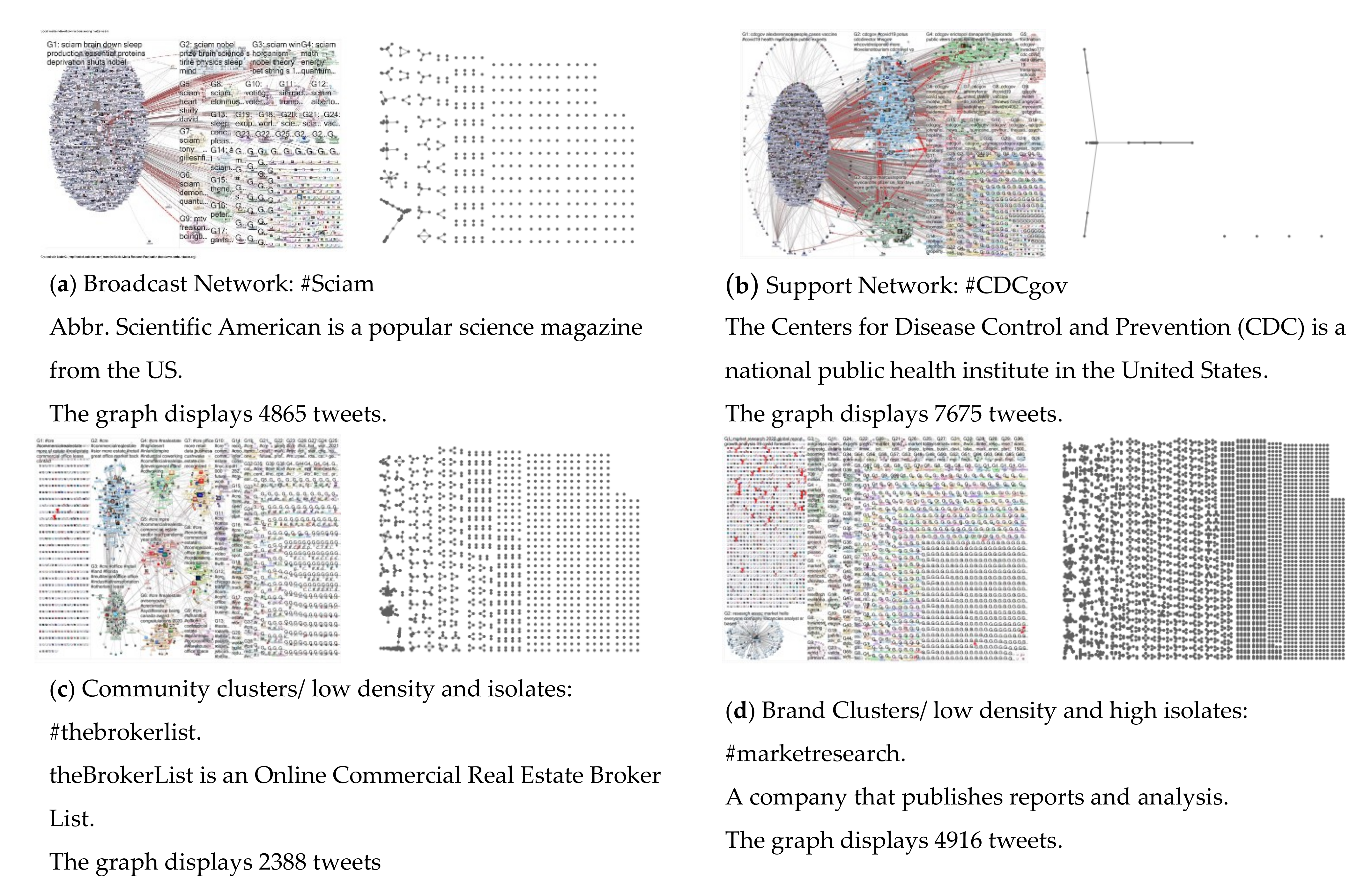
Information flow is influenced by the network structures, and to explore it, several network values have been defined, such as density [31], modularity [32], centralization, and the number of isolates. Research performed by [27] was based on combining these measurements into one analysis, and its conclusion has established six basic topological structures that appear on Twitter. These structures can be polarized, community, tight crowd, brand, support, and broadcast networks.

2.1. Types of Topic Structures

Polarized topologies are characterized by high density and high modularity. The best example of this is the debate, and high conflict manifested when talking about the two political parties in the USA, the Democratic Party and the Republican Party. Participants/members of one of these groups interact almost exclusively with internal group members, rarely discussing and contacting the other group, which reinforces group homogenization and topology polarization. This stark division provides an opportunity for brokers who occupy structural holes [33] and bridge these divided clusters to have a significant role.

The tight crowd topology is similar to the previous one since it has high density but low modularity. Clusters of this topology are highly interconnected and often overlap one another. Modularity is not as distinct as in the previous situation, enabling more differences and a higher number of subgroups, again with similar being connected.

Brand topologies have a low connection density with a high number of isolates. Individuals within these clusters usually discuss with others from the same cluster. Topics are usually regarding brands, songs, movies, etc.

Community clusters have low density and a low number of isolates compared to the previous topology. Like real communities, groups discussing the same topic can have similarities and differences and can differ in size. Individuals that are information hubs are common, and information sharing is democratized.

Broadcast and support topologies are characterized by high centralization; they differ according to the information sharer’s position and information flow direction. If information flows outwards from the central, most connected node, then the node is likely a news outlet or a celebrity. If the information flow is towards the central one, then that node is likely customer service of a company because people present it with their problems and questions. 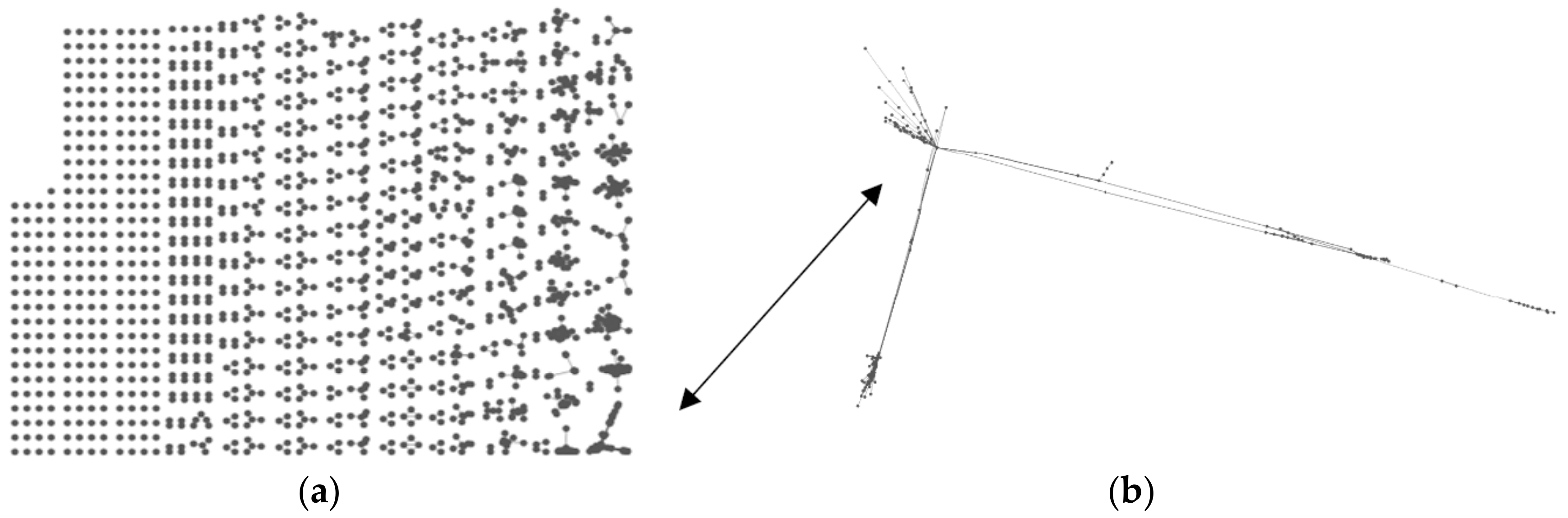Figure 1 shows the six types of network topic topologies presenting tweets collected during a certain period. The left pair of each figure is plotted using the NodeXL MS Excel add-in and shows directed graphs with nodes grouped by cluster using the Clauset–Newman–Moore cluster algorithm. The graph was laid out using the Harel–Koren Fast Multiscale layout algorithm. There is an edge for each “replies-to” relationship in a tweet, an edge for each “mentions” relationship in a tweet, and a self-loop edge for each tweet that is not a “replies-to” or “mentions”. The right pair of each figure presents the sum of individual clusters that make the dataset. Node relationships and weights determine cluster shapes. They are plotted using the default MATLAB R2018a plot function, which plots clusters based on their size, sorted largest (bottom left) to smallest (top left), which creates their axis placement.

Each twitter dataset (network) is classified as one of these topic topologies. All of them are formed from individual tweets (nodes) in a communication relationship (edges) with others and since distance on the internet is abstracted. A cluster is formed if a user is connected with at least one user; if not, users are isolated and depicted as a single node. Repeated cluster patterns are seen because of the limited relationship possibilities, especially with fewer nodes. For example, there is only one way to connect two nodes; they must form a line cluster, while three nodes can create a triangle or a three-node line cluster. These patterns are seen more often when any communication between nodes (including back and forth) is seen as a single relationship, which will be the focus of this paper.

2.2. The Procedure of Classifying Twitter Topic Networks

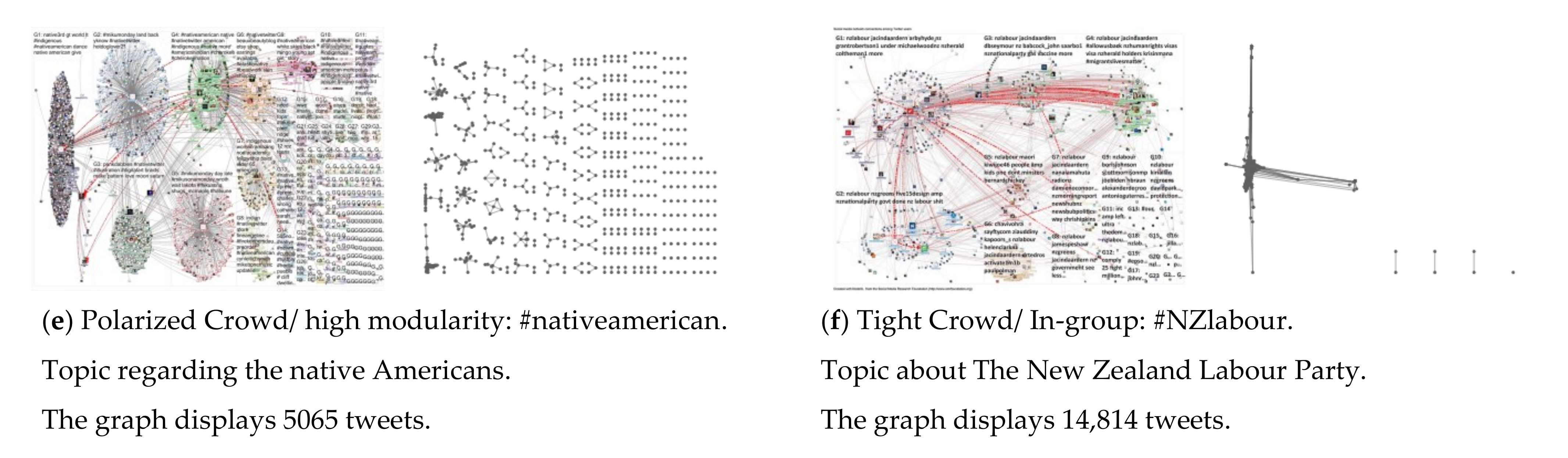
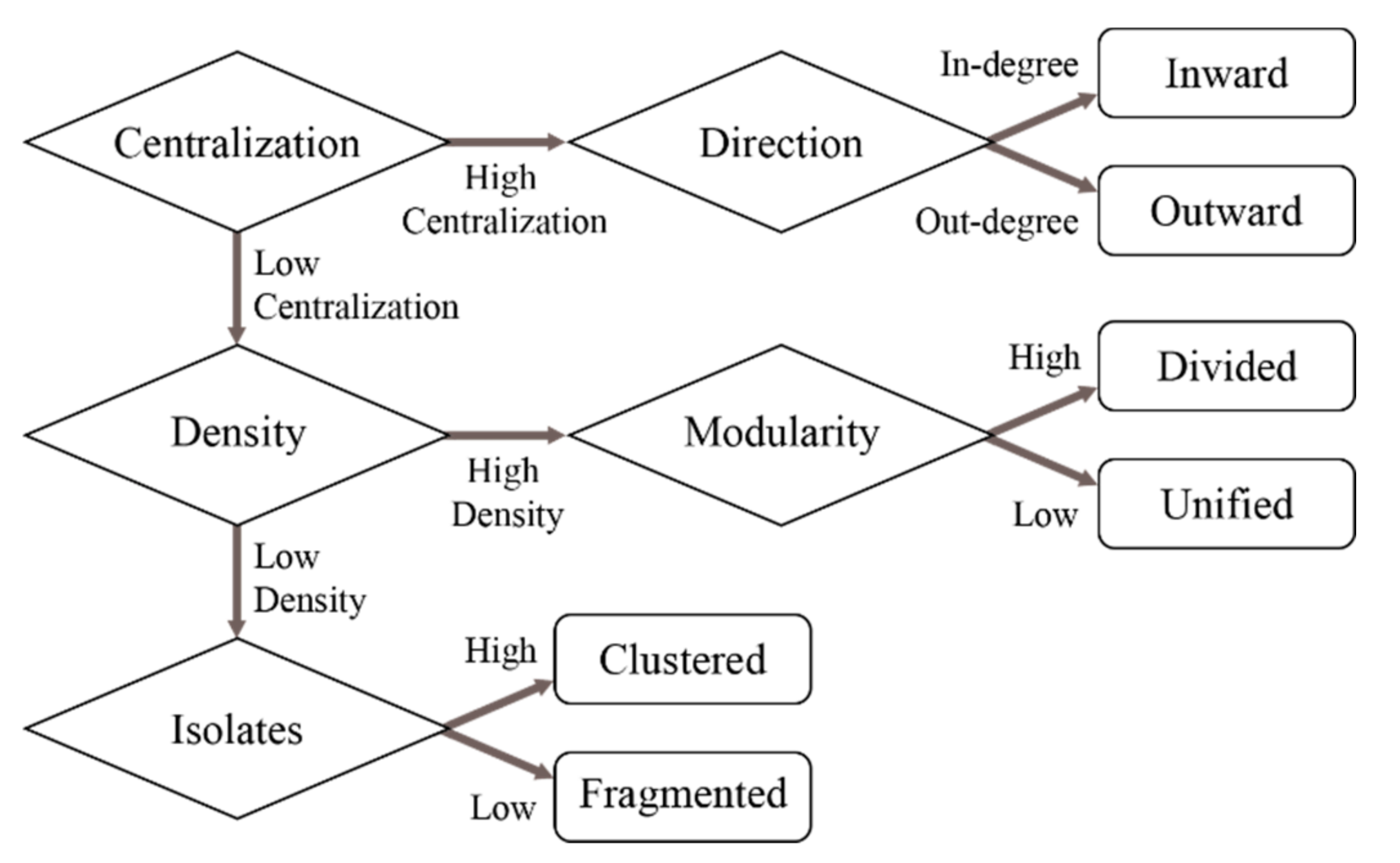
The manner of topic identification is a step-by-step classification process. Datasets that have been classified are exempt, and the unidentified networks progress further; as shown in Figure 2, the process stops when all networks are identified. The initial classification is performed to find the highly centralized networks. As proposed by [27], a scree plot is used to determine the threshold between low and high values since mean, first, and third quartile or median values are unsuitable. Figure 3 shows the initial significant drop point; datasets with higher values are considered highly centralized and are scrutinized for their direction of information flow to determine whether it is inwards or outwards oriented. The rest of the classification process is based on mean values being the threshold for defining high and low values.

The second step focuses on networks with low centralization; they are checked for network density to determine whether it is high or low. This threshold factor is obtained by calculating the mean graph density values of all datasets. If the graph density of the observed dataset is higher than the threshold value, then it is a highly dense network. The same threshold principle is used to determine networks with high/low modularity.

Low-density networks are checked for their number of isolates. A threshold value is obtained as in the previous by calculating the mean isolate values of all datasets and classifying them according to their higher/lower threshold values.

Classification based on centralization values is the initial step; the procedure ends when all datasets are classified.Out of the n = 162 datasets, there are n = 45 inwards oriented highly centralized datasets while n = 21 are outwards oriented. Centrality values show mean values (M) at 0.9026 with a standard deviation (SD) of 0.0809 and range from 1 to 0.7549. Other datasets with low centralization values are next checked for their density based on the mean threshold: M = 0.0046 with SD = 0.0072. Datasets that are determined to have high density are checked for their modularity, with those that have greater modularity than M = 0.46 with SD = 0.1457 being classified as having high modularity (n = 16) while the rest have it low (n = 12). This leaves the other datasets as low density where the threshold mean is M = 354.75 with SD = 519.67 with n = 19 high isolated and n = 49 low isolated datasets. It is important to note that the cutoff points in this paper are based on this specific set of networks and may vary across other networks.

3. The Procedure of Classifying Clusters

Researchers have previously analyzed how and why the same relationships keep appearing. They have implemented various models to capture these regularities to define their distribution tendencies. A seminal work [34] applied statistics to social networks. The results showed strong reciprocity meaning that there are tendencies for repeating the same relationships. Frank and Strauss [35] defined Markov dependence in which a possible tie from node $i$ to node $j$ is assumed to be contingent on any other possible tie involving $i$ or$j$, even if the status of all other ties in the network is known. Markov dependence can be characterized as the assumption that two possible network ties are conditionally dependent on a common actor. The Markov random graphs are one class of exponential random graph models which are statistical models for expressing structural properties of social networks observed at one moment [36]. They can describe various structural tendencies that define complicated dependence patterns that are not easily modeled by more basic probability models.

Exponential random graph models have the following notions and are expressed in the form (1) [37]. They describe a general probability distribution of graphs with $n$ nodes; the summation is over all configurations of A. Any random graph is represented by its adjacency matrix $Y$ with elements $Y_{ij}$. Graphs are non-directed, i.e., $Y_{ij}=Y_{ji}$ holds for all $i,j$. Elements (nodes) are $i$ and $j$ which are members of a set $N$ that has $n$ actors. A random variable $Y_{ij}$ exists where $Y_{ij}=1$if there is a tie between actors $i$ and $j$ and if there is no tie $Y_{ij}=0$. We do not account for self-ties, meaning $Y_{ii}=0$ for all $i$.

$$Pr\left(Y=y\right)=\left(\frac{1}{k}\right)exp\left\{{\displaystyle \sum }_A\eta AgA\left(y\right)\right\}$$

(1)

So that $\eta A$ is a parameter corresponding to configuration $A$, it is non-zero only if all pairs of variables in $A$ are conditionally dependent. Next, $gA\left(y\right)={{\displaystyle \prod }}_{y_{ij}ϵA}{y}_{ij}$ is the network statistic corresponding to configuration $A$, $gA\left(y\right)=1$ if the configuration is observed in the network $y$ and is 0 if otherwise. Finally, $k$ is a normalizing quantity that ensures (1) is a proper probability distribution. $\frac{1}{k}$ is generally thought to be a very small number, reflecting the very low probability that any random graph (even if a good fit) will be identical to any observed graph; for all but the smallest networks, the value of $k$ is intractable to calculate [38].

Note that communication topologies are representations of relationships between nodes (individuals) and can be expressed in the form of $Y_{ij}$. They can depict clusters or datasets. On the other hand, communities in social networks represent a set of individuals that are interested in or discuss the same/similar topic. This is not to be confused with community clusters (characterized by low density and low isolates) as a Twitter topic-network, as defined by [27].

The focus of this paper is the identification of the repeated shapes based on datasets acquired from the NodeXL Graph Gallery, a web repository for social media network data. The data is processed by our customized application that extracts the tweets, retweets, mentions, and replies relationships from the dataset. Tweets are treated as nodes (vertices: $V$) and their relations as links (edges: $E$). Tweets that are connected in any of the previous ways are treated as a cluster and are represented by a graph in the form of $G=\left(V,E\right)$. Any type of relationship is treated as a single one making the graph undirected, which is a common practice in Twitter network analysis [39,40]. Each cluster of a dataset is checked individually for its shape by analyzing its four traits through a screening process. The first trait is the total number of nodes of a cluster $V_c$ which is calculated by using the following formula:

$$V_c={\displaystyle \sum }_{v\in G}v$$

(2)

The second feature is based on calculating centrality measures for each node [12,27,31]. The first is the degree centrality which is the simplest form of centrality and is calculated by counting the number of edges connecting to each node. It shows one’s direct exposure to the network and presents the opportunity for direct influence over others. To calculate it for each node, we use:

$${\displaystyle \sum }_{v\in V}\mathrm{deg}\left(v\right)=2\left|E\right|$$

(3)

On Twitter, this centrality is based on ties a user has established with others when retweeting or mentioning that user. Next, we check for the betweenness centrality $\left(C_B\right)$ which is calculated according to the shortest path between other users’ paths and is the earliest type of social network analysis approach [41]. A node ($v$) has a high value of betweenness centrality when it can be a bridge node on many shortest paths that connect pairs of nodes in the network, conversely higher amounts of shortest paths running through a node mean a higher betweenness value. The node with the highest value can be seen as a gatekeeper of the network; it is also a liaison between clusters of a group. To measure it, we use:

$$c_B\left(v\right)={\displaystyle \sum }_{i\ne v\ne j\in V}\frac{{\sigma }_{ij}\left(v\right)}{{\sigma }_{ij}}$$

(4)

So that ${\sigma }_{ij}$ presents the total number of shortest paths between node $i$ and node $j$; and ${\sigma }_{ij}\left(v\right)$ denotes the number of those shortest paths between $i$ and $j$ that pass-through node $v$. Nodes that are connected only with a single connection have $\mathrm{deg}\left(i\right)=1$ and $c_B\left(v\right)=0$ while isolated nodes have $c_B\left(v\right)=\mathrm{deg}\left(i\right)=0$.

The third identification feature is based on determining how many node types a cluster has. A single node type ($T_k$) consists of all nodes that have identical degree values and betweenness values:

$$T_k=\left\{\begin{array}{c}{c}_B\left(i\right)=c_B\left(j\right)\\ \mathrm{deg}\left(i\right)=\mathrm{deg}\left(j\right)\end{array}\right.$$

(5)

where $k$ stands for the ordinal and includes nodes $i$ and $j$ note that degree and betweenness values among themselves do not need to be identical. Thus, the total number of node types is obtained when summing all different types of nodes.

The fourth identification feature determines whether a cluster has an open or closed structure; this is a true or false statement (Boolean value) and is checked by each node’s degree and betweenness centrality values. We consider clusters to be closed if all of their nodes are connected to at least two other nodes, which means they communicate with others within that cluster; closed clusters do not have weak influencers. A cluster $C$ is considered open if it has at least one node $v$:

$$v \in C, so that \mathrm{deg}\left(v\right)=1 and c_B\left(v\right)=0$$

(6)

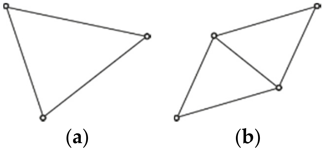
If the cluster does not have any of these nodes, then it is a closed cluster. Examples of closed clusters can be found in Figure 4a,b and Figure 5c.

3.1. Identification Traits of Fixed Shapes Clusters

For simplification purposes, authors chose picturesque names for shapes they defined, such as the circle, chain, the Y, and the wheel [13]. For the same purpose, we have given names to the most common communication topologies. Our primary cluster differentiation is based on their structure, which can be fixed or variable. Clusters with fixed structures do not change shape; their node arrangement follows exact rules and can be identified using the degree and betweenness centrality values found in

Table 1. Centrality values of fixed clusters.

	Number of Nodes	Type of Centrality	Value
Isolates	1	Degree and betweenness	0
Triangle	3	Degree	2
-	3	Betweenness	0
Square diagonal	2	Degree	2
-	2	Degree	3
-	2	Betweenness	0.5
-	2	Betweenness	0

.

Figure 4 shows graphical depictions of fixed shapes from Table 1.

3.2. Identification Traits of Variable Shaped Clusters

Topologies with variable structure follow a mathematical rule and do not have a limitation to the number of nodes, as long as the rule applies. These rules or standards help define elements as identical; therefore, it is possible to use the logic of node types. Next, we will explain how to identify clusters with variable structures whose shapes are shown in Figure 5 with Figure 5a shows line clusters that are defined by having two nodes $\left(i,j\right)$ that are located on opposite ends of the cluster, creating a single line cluster.

$$C_{line \left(single\right)}=\left\{\begin{array}{c}{V}_c=2 \\ \mathrm{deg}\left(i,j\right)=1, c_B\left(i,j\right)=0\\ T_k=1\end{array}\right.$$

(7)

Among these end nodes, there can be any number of nodes ($v$) so that a longer line cluster is created:

$$C_{line \left(multi\right)}=\left\{\begin{array}{c}{V}_c\ge 2 \\ \mathrm{deg}\left(i,j\right)=1, c_B\left(i,j\right)=0\\ \mathrm{deg}\left(v\right)=2 \\ T_k=2\end{array}\right.$$

(8)

While $\mathrm{deg}\left(v\right)$ is fixed betweenness values of nodes $v$ are variable and depend on the length of the cluster. Note that line clusters with two nodes have a single node type; for simplification purposes, we choose to make an exception to the node type identification rule.

Simple star clusters (Figure 5b) have one central node $\left(i\right)$ which is connected to all (any number) of other nodes ($v$) with a single edge while other nodes are not mutually connected. Node $i$ is not connected to itself. The minimal number of nodes this type of cluster has is four since, with three nodes, it will be classified as a line cluster. Thus, we have:

$$C_{simple star}=\left\{\begin{array}{c}{V}_c\ge 4\\ \mathrm{deg}\left(i\right)=V_c-1 \\ \mathrm{deg}\left(v\right)=1, c_B\left(v\right)=0\\ T_k=2\end{array}\right.$$

(9)

All noncentral nodes ($v$) are identical, meaning that there are only two node types. Only the central node has a case-by-case variable degree and betweenness values, while these values of other nodes are fixed to 1 and 0, respectively.

Complex star clusters (Figure 5c) have more than four nodes and are characterized by having closed networks since they do not have nodes $\left(v\right)$ with the degree and betweenness values of 1 and 0, respectively. Another identification feature is that they have two types of nodes, therefore:

$$C_{complex stars}=\left\{\begin{array}{c}{V}_c\ge 4 \\ \mathrm{deg}\left(v\right)=1, c_B\left(v\right)=0\notin C\\ T_k=2\end{array}\right.$$

(10)

Preferential attachment (Figure 5d) networks are characterized by a few “hubs” that have a greater number of connections, whereas all other nodes have fewer [42]. Therefore, they possess hub nodes $\left(v\right)$ with a variable degree and betweenness values together with end nodes $\left(i\right)$ with degree and betweenness values being 1 and 0, respectively:

$$C_{PA}=\left\{\begin{array}{c}\mathrm{deg}\left(v\right), c_B\left(v\right)\in Z\\ \mathrm{deg}\left(i\right)=1, c_B\left(i\right)=0\\ T_k=1+T_{k\left(v\right)}\end{array}\right.$$

(11)

The key identification feature of these networks is the integer nature of their degree and betweenness values since their “branches” do not interconnect. If this were not the case, their betweenness values would have been noninteger. The total number of node types $\left(T_k\right)$ is equal to the number of different hub nodes $\left(T_{k\left(v\right)}\right)$ plus 1, which stands for the end node type $\left(T_{k\left(i\right)}\right)$.

Figure 5e shows windmill clusters that are made up of a triangle with any number of nodes connected only to one of its vertices; these non-triangle nodes are not mutually connected; therefore, we have:

$$C_{\mathrm{windmill}}=\left\{\begin{array}{c}\mathrm{deg}\left(v\right)=V_c\\ \mathrm{deg}\left(i\right)=1, c_B\left(i\right)=0\\ \mathrm{deg}\left(j\right)=2, c_B\left(j\right)=0\\ T_k=3\end{array}\right.$$

(12)

There are three types of nodes in this cluster; the first includes a single node connected to all other nodes $\left(v\right)$, thus identifying its degree value equal to the number of nodes. The second type $\left(i\right)$ are end nodes with degree and betweenness values of 1 and 0, respectively. The third type $\left(j\right)$ includes two nodes that conform to the triangle cluster definition, meaning their degree and betweenness values are 2 and 0, respectively.

Figure 6 shows the cluster identification flowchart based on which the algorithm is created. It initially treats all datasets and topologies as 100% unidentified and screens each of their clusters to determine their four identification traits. The process starts by identifying and counting isolated nodes and subsequently removing them from the dataset.

We note that there are some distinctions between random clusters. The first subgroup of random clusters are topologies that can be defined using the proposed four-step filtering process. Since their presence in the overall results is less than 1%, we declare them as random. An example of this cluster type can be seen in the top part of Figure 5f. The second subgroup is clusters that follow a truly random setup [43], as seen in the middle part of Figure 5f. The third subgroup of random clusters can be viewed as two or more conjoined clusters, shown last in Figure 5f, where we see the simple and complex stars merged into one cluster. Since there is much subjectivity in this type of cluster identification, we observe them as a single cluster.

4. Findings

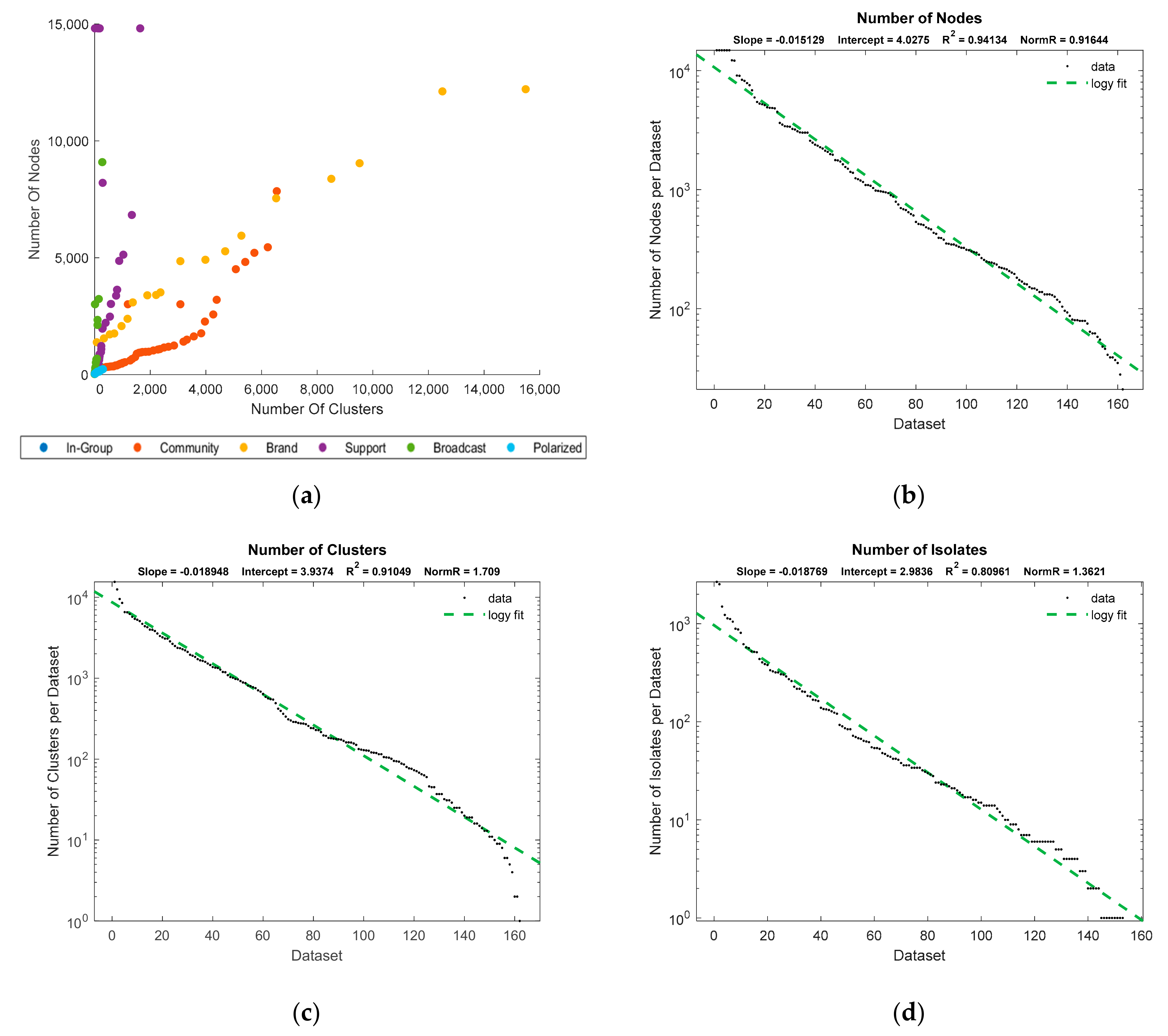
For this study, we analyzed 162 twitter datasets obtained from the NodeXL database. The total number of tweets in these datasets was 334,762, of which 26,814 tweets were not retweeted or communicated with even one time, leaving them isolated in the network. Other tweets were located in one of the 24,434 clusters. Our methodology for cluster identification identified 89.6% cluster shapes while the rest categorized as unidentified or random clusters. Dataset metrics and distributions can be seen in Figure 7.

As seen in Figure 7a, our classification process pointed out the cluster to node relationship tendencies across different topologies. We saw that with a higher number of nodes, networks tend to manifest in the form of broadcast and support topologies with a limited number of clusters. The majority of their nodes must be positioned within a single main cluster, where a node is broadcasting and/or receiving information, such as CNN. Due to a finite number of nodes in each topology, the leftover nodes form only a relatively small number of clusters. When more nodes are added, which are not connected to the main cluster, the topologies evolve into the brand or community type that had a high number of clusters and nodes.

This process is defined seen as the evolution of social and communication networks [10]. Groups can expand by drawing in new members or contract when losing members. Groups can also merge into a single one, while large social groups can be divided into several smaller ones. Finally, new communities can be created while old ones may disappear.

Figure 7a shows that in-group and polarized topologies had fewer tweets, and we found them to be the most elusive topologies. The in-group is characterized by high graph density and low modularity, which means that adding new individuals could form a new cluster. This would increase the modularity and evolve the topology into the community one. The second for their elusiveness is that a node can become highly influential over time, so the topology evolves into the centralized one.

Polarized topologies follow the principle; it is difficult to find a low number of clusters that are mutually well connected but at the same time do not evolve into a highly centralized topology. The second option is that more clusters are singled out (added or extracted), so the topology becomes community-based (low density and low isolates). As pointed by [27], degree centralized (support networks) are more often found compared to the out-degree (broadcast) networks, which was our finding as well.

4.1. Identifying the Most Common Cluster Shapes

Since datasets are of different shapes, types and have different numbers of nodes, the best way to unify their results is by observing them percentage-wise. Therefore, the number of weak influencers is expressed as a percentage of the total number of nodes, while the cluster shape percentages are calculated based on the total number of clusters.

Table 2. Results of cluster analysis and their repetition across different topic topologies.

	Weak Influencers (%)	Total Nodes	Isolates (%)	Line (%)	Triangle (%)	Star (%)	PA (%)	Square (%)	Complex Star (%)	Windmill (%)	Random (%)
Total
Max	94.42	14,814	37.33	88.06	25	50	20	20	37.5	33.33	100
Min	0.17	21	0	0	0	0	0	0	0	0	0.64
Avg	57.11	1827.83	9.55	54.25	3.32	14.04	2	1.75	2.04	1.5	23.18
Std	17.36	2050.21	5.07	19.39	4.48	9.42	3	2.67	3.74	3.58	17.35
In-group (High Density/Low Modularity)
Max	81.51	380	15.97	73.08	25	46.15	20	20	11.11	5.56	40
Min	38.64	35	2.03	20	0	4.35	0	0	0	0	4
Avg	58.49	151.5	8.01	54.16	4.13	21.46	2	2.35	1.39	1.16	16.34
Std	13.4	108.33	4.23	18.67	7.72	10.69	6	5.78	3.45	2.12	11.46
Community clusters (Low Density/ Low Isolates)
Max	91.25	7847	27.97	88.06	6.61	38.89	11	5.26	7.14	7.04	21.69
Min	14.21	130	3.6	47.93	0	3.77	0	0	0	0	2.99
Avg	68.49	1417.86	11.68	63.79	2.57	18.1	3	1.69	1.84	1.16	8.65
Std	13.64	1650.55	7.37	9.47	1.91	7.56	2	1.4	1.73	1.5	4.16
Brand clusters (Low Density/ High Isolates)
Max	94.42	12,210	37.33	87.83	4.95	16.56	4	3.68	3.62	2.28	8.59
Min	58.05	1385	8.61	63.75	0	6.51	0	0	0	0	0.64
Avg	75.12	4977.95	22.21	77.01	2.55	11.61	2	1.38	0.92	1.14	3.71
Std	9.56	3418.67	8.47	7.25	1.51	2.61	1	0.91	0.91	0.69	2.17
Support (Inwards facing high centralization)
Max	80.71	14,814	13.49	85.71	12.5	50	17	3.33	5	33.33	100
Min	0.18	48	0	0	0	0	0	0	0	0	1.3
Avg	40.75	3195.69	3.59	50.28	1.71	9.8	1	0.38	0.37	1.78	35.39
Std	22.9	4957.19	3.39	31.1	3.18	11.8	3	0.86	0.98	5.57	36.96
Broadcast (outwards facing high centralization)
Max	87.48	9090	6.25	71.43	25	50	7	5.56	21.43	33.33	100
Min	0.17	21	0	0	0	0	0	0	0	0	4.44
Avg	44.35	1099.71	2.23	29.88	2.4	10.21	1	0.42	1.36	1.92	55.38
Std	21.57	2099.87	1.68	28.4	6.06	15.74	2	1.37	4.76	7.28	38.73
Polarized (High Density/ High Modularity)
Max	81.61	235	19.54	76.92	16.67	33.33	12	16.67	37.5	12.5	38.89
Min	9.33	39	1.33	5.56	0	0	0	0	0	0	3.85
Avg	55.46	124.25	9.59	50.39	6.54	13.05	2	4.29	6.33	1.85	19.63
Std	23.11	66.65	5.28	21.42	6.51	8.09	4	5.69	10.63	4.31	10.59

shows average values of shapes and nodes within datasets, with the first part showing the average values across all datasets while others are specific to twitter topics and their topologies. Starting with the variable-shaped clusters, the most common shape is the line cluster averaging 54.25% across all datasets, which comes from the low isolate topology. From

Table 3. Sizes of variable clusters.

	Line Cluster	Simple Star	PA	Complex Star	Windmill	Random
Max	6	459	303	108	38	13,461
Min	2	4	5	5	4	4
Avg	2.27	6.88	10.79	8.05	4.85	253.49
Std	0.09	8.9	11.72	3.31	2.75	552.42

, we see that the average length of line clusters is 2.27 nodes, with a maximum of 6 consecutive nodes.

The second most common cluster shape was random (23.18%); they were primarily found in broadcast (outward centrality) topologies (55.38%) since they have a single cluster with a large number of nodes which means a high chance of being random. Random clusters were found the least in the highly isolated (brand) support topologies averaging 3.71% because the high number of isolates leaves a small number of nodes to be mutually connected.

Simple star clusters are third, taking up 14.04% of all cluster shapes. These clusters point to individuals sharing information among a close number of people that do not get it from somewhere else or share it further; the highest number of these individuals is 459 found in the community cluster topology.

Other variable shapes such as the PA, complex star, and windmill make up less than 3% of all cluster types, with PA clusters being the most common in the inwards centrality topologies with the largest one having 303 nodes. Complex stars appeared most often in community networks that have low density and isolates, with the largest one having 108 nodes. Regarding the fixed-shaped clusters, the triangle cluster appeared the most often in the broadcast topology (6.54%), while overall, it appears 3.32%. The square cluster can be found 1.75% of the time, and it most often appears in highly modular topologies with 4.29%.

4.2. Size Distribution of Common Clusters

Table 3 shows the sizes of variable clusters by considering the maximum and the minimum number of nodes found in the cluster type. Shown also are their average length and standard deviation to determine how often they change shapes.

4.3. Participation of Low Influencers

Low influencers are users who talk or share a link about a particular subject but are isolated since their tweets are unanswered or not retweeted. Research [26] point to their importance even though they do not attract the attention of others. They contribute to the overall discussion on the topic since their followers can see what they posted on their walls, thus prompting them to comment. The definition points to two types of weak influencers that can be differentiated based on their degree and betweenness values: those within clusters (values of 1 and 0 respectfully) and isolated ones (values of 0 and 0 respectfully).

Weak influencers were, on average, most commonly found in the brand (high isolate) topology, where they average 75.12%, with the maximum amount being 94.42%. The same topology hosts the maximum number of isolated influencers (37.33%), and they were most commonly found there at 22.21%. We found that weak influencers in centralized topologies form a random cluster resembling a simple star shape where all nodes were connected to a single central node. Users, in this case, are acquainted with the main node (broadcaster) and are not communicating among themselves. An example of this main node is CNN, as shown in Figure 8.

4.4. Overall Influencer and Cluster Size Distribution

Power laws are frequencies of distribution of various elements where the majority are small (accounting for the element’s scale) while very few of them are large. Power laws (such as Pareto and Zipf) apply to everything from city sizes to word frequencies. An important finding regarding social media and influencers Nielsen’s [7] approximation of influencer distribution to be 1-9-90. The 1% of the participants in an internet community generates the majority of content. Next, the minority of the content is produced by 9% of participants, while 90% of people are passive and do not participate in discussions. When comparing the rule with Zipf’s Law findings, both provide a means of describing the distribution in the engagement of members by post frequency, but Zipf’s law offers a more precise description of the data [28]. Following the same principle, we check all nodes and clusters from our dataset to see whether power laws apply.

Figure 9 shows the total distribution of cluster sizes, degree and betweenness values across all datasets. Displayed are 24,434 clusters, 88,890 data points representing degree centrality values, and 251,776 data points for betweenness centrality. The degree centrality values of nodes were well fitted to the curve and conform to the power law. As for the cluster size distribution, the initial deviation from the curve is caused by large clusters that are not following the same size progression as others. Since there are only a few of them, the rest of the clusters with smaller sizes conform to the power law. The same goes for the betweenness centrality in addition to the lowest numbers.

Note that the subgraphs are different due to the equations used for their calculation. For example, each added cluster in Figure 9a is independently added to the graph and does not influence other clusters. Figure 9b shows that a newly added node to a cluster changes the degree values only of those nodes it is connected to. In Figure 9c, each added node to a cluster impacts the betweenness values, shortest paths of all nodes in that cluster.

5. Discussion

Our discussion will focus on two areas: the first will evaluate the implications of cluster shapes and human behavior patterns. The second will analyze the general human behavior and reasons why said shapes/patterns appear.

5.1. Cluster Shapes and Implications on Human Behavior

Simplicity implies repetition. Individuals rarely enter large-scale discussions; they often have dialogues with others, as shown by the prevalence of line clusters. Additionally, numerous participants prefer to voice their opinion about a topic disregarding the general sentiment, which can be seen through large numbers of isolated users, especially regarding brands. This rule exists in various natural systems; the most abundant element is hydrogen, followed by helium [44], while the most abundant lifeforms are viruses [45].

Other researchers came up with similar conclusions by observing multiple datasets regarding the same topic, these being “TV/shows”, “soccer/sports”, “politics/breaking news”, etc. For example, topics regarding TV/Shows have a greater average tweet rate than other topics; however, its retweet rate is lower [8]. This corresponds to our brand topology findings where tweets without retweets are seen as isolates. On the other hand, the retweet rate and the number of links are significant for “soccer/sports” and “politics/breaking news” topics which implies discussions [8]; consider Figure 8, where CNN is the information source for politics/breaking news.

There are rules to large random clusters. Due to many participants and connections between them, large clusters are most likely random; putting their names aside, there are underlying rules. This is evident in the shape of clusters centralized around Twitter accounts of Scientific American, CDC, CNN, shown in Figure 1 and Figure 8, when observing the organized direction of relationships with said accounts. These highly centralized clusters tend to attract participants and other clusters to merge with them, resulting in their dominance and transforming them into broadcast and support network topologies. Additionally, these clusters follow power laws where the central node is the dominant one [26].

There are exceptionally dominant individuals but are they legitimate? As previously shown, influencers are often highly centralized within a cluster, with that cluster being randomly shaped. Individuals in simple star clusters can be considered uncontested influencers because participants only communicate with them; no side communication is performed since it would contradict the Equation (9). This can be used to create a methodology for detecting spam accounts since long-term single-direction communication is unlikely. Another oddity to consider is that the chain of tweets/retweets can be unbroken for a considerable period, as seen with the largest PA having 303 nodes.

All participants can be important and their opinions influential, most often seen in community networks that do not have a central information hub meaning that their discussions are democratic. They are usually formed around conferences, events, or discussions indicating multiple activity centers, each with its audience, influencers, and sources of information [27]. The egalitarianism of such communities can be seen through the prevalence of complex stars, triangle and square diagonal topologies characterized by including each individual in the discussion. Due to the prevalence of square diagonal, triangle, and windmill clusters, we conclude that they are a common precursor to other larger clusters whose temporal evolution will be examined in our future work.

5.2. Broader Individual Behavior Considerations and Explanations

Artificial topologies, for example, in computer science, are usually organized into eight basic topologies: point-to-point, bus, star, ring or circular, mesh, tree, hybrid, or daisy chain [46]. They can evolve and change shapes over time and receive/lose nodes [10]. They can be created and managed by a single entity, such as a network manager. Social networks are decentralized and more democratic; they are defined and influenced by their users, making them act like swarms of bees or schools of fish.

Even though social behavior and communication are complex, some regularities in topologies appear and influence their formation. The first reason is homophily, where individuals with similar characteristics are more likely to form friendships; in other words, birds of a feather flock together [47]. These features can be gender, race, age, and other observed characteristics. The second reason lies in transitivity, where if two unconnected actors are connected to a third actor, at some point, a tie will be formed between them. Chances of transitivity are greater if the actors have the same features, as defined by homophily. Research points to the importance of distinguishing between transitivity and homophily as drivers of clustering in networks. If transitivity has greater influence, then outside interventions can have long-run effects on network structure.

On the other hand, if homophily is the primary force for clustering, outsider matching interventions are less likely to lead to durable changes in network structure [48]. Knowing how and why people connect can help influence viral advertising [26], marketing campaigns [49], or societal behavior [50]. By implementing the same principles, spam, bots, fake news, and hate speech can be identified and eliminated [19].

When it comes to group behavior, two main explanatory concepts emerge independence and saturation. Independence refers to the degree of freedom with which individuals function in a group [13]. Besides the influence of other individuals, one’s independence is affected by the accessibility of information, “noise”, reinforcement, kind of task, and by the person’s perceptions and cognitions regarding the overall situation [14]. Lower independence limits possibilities for action/performance and influences the persons’ willingness to perform at their optimum level, leaving them uninterested in further participation [14]. Saturation refers to the total number of information transfer requirements placed upon a user in a given position in the network [51]. The effectiveness of a group acts inversely with saturation: with greater saturation, the group is less efficient.

When looking at the shapes of clusters, we can make assumptions about the information flow in them. Early experiments showed that communication patterns imposed upon a group are an important determinant of group behavior [52]. Individuals that are well informed may emerge as cluster narrative leaders and can control the flow of information while the others gather around them, creating a centralized topology. As new members are added, the cluster shapes can change. Research has shown that centralized groups have higher speed and efficiency in information transfer [53]. The same groups can be unstable; if the centralized actor is disconnected, the information flow is reduced, and the cluster stability is endangered [27]. Groups exhibit interdependence, meaning they share a common purpose and a common fate. They also have specific identities which lay the foundation for that group. Users do not communicate the same way constantly; they change their style according to the topic and other participants. Activities, and lack of thereof, often depend on the context instead of it being an individual trait [24,54].

All users have joined the network at some point in time and were equal; the question is why some users grow their influence more than others? One of the answers lies in trust, which is the single most crucial element that gave rise to the trend of influencer marketing [55]. Influencers can impact social media conversation and subsequent behavior regarding brands or topics [56]. Areas of their influence may be commercial, interactive, reciprocal, and disclosive. Influencers define the “1-9-90 rule”, which aligns with Zipf’s law and other power laws.

6. Conclusions

Even with all the freedom, decentralization, and democracy, people’s behavior falls under repeated patterns. To define these self-organized patterns and find how often leaders and followers appear, we have implemented datasets obtained by using NodeXL. Our topical, not general, network observation allows us to observe users organized in clusters that can be disconnected from one another; additionally, this allows the existence of isolated users.

We found that two main group types can be differentiated according to their structure: fixed and variable. Apart from the isolated users, we defined the fixed clusters as a triangle or a square with a single diagonal. The variable shapes are simple and complex star clusters, preferential attachment clusters, line, windmill, and random clusters. We defined their size variations and frequency of appearance in general and according to topic networks. We found that power laws do apply for the influencer connection distribution (degree centrality) and a cluster size distribution while the betweenness centrality is exponentially distributed. The simplest cluster forms are repeated more often than complex ones, thus meaning that simplicity implies repetition. There are rules to large random clusters; most of them become centralized as their size increases resulting in a broadcast/support topology.

There are a few limitations to our research, one of them is that our focus was limited to the six most common Twitter topic networks, and there are more possible options [27]. Secondly, the methodology in this paper described 90% of all cluster shapes. Using the same methodology, we identified and described other cluster shapes, but since each type appears rarely, less than 1% overall, we disregarded them. Finally, the cutoff points are based on datasets used in this paper and may vary across other ones.

Our future research will incorporate these topologies and will be focused on finding others. We will also observe underlying patterns of other social networks, such as Facebook, Instagram, LinkedIn, and compare them to Twitter.