Greed Is Good: Rapid Hyperparameter Optimization and Model Selection Using Greedy k-Fold Cross Validation

Abstract

Selecting a final machine learning (ML) model typically occurs after a process of hyperparameter optimization in which many candidate models with varying structural properties and algorithmic settings are evaluated and compared. Evaluating each candidate model commonly relies on k-fold cross validation, wherein the data are randomly subdivided into k folds, with each fold being iteratively used as a validation set for a model that has been trained using the remaining folds. While many research studies have sought to accelerate ML model selection by applying metaheuristic and other search methods to the hyperparameter space, no consideration has been given to the k-fold cross validation process itself as a means of rapidly identifying the best-performing model. The current study rectifies this oversight by introducing a greedy k-fold cross validation method and demonstrating that greedy k-fold cross validation can vastly reduce the average time required to identify the best-performing model when given a fixed computational budget and a set of candidate models. This improved search time is shown to hold across a variety of ML algorithms and real-world datasets. For scenarios without a computational budget, this paper also introduces an early stopping algorithm based on the greedy cross validation method. The greedy early stopping method is shown to outperform a competing, state-of-the-art early stopping method both in terms of search time and the quality of the ML models selected by the algorithm. Since hyperparameter optimization is among the most time-consuming, computationally intensive, and monetarily expensive tasks in the broader process of developing ML-based solutions, the ability to rapidly identify optimal machine learning models using greedy cross validation has obvious and substantial benefits to organizations and researchers alike.

1. Introduction

Organizational development and adoption of artificial intelligence (AI) and machine learning (ML) technologies has exploded in popularity in recent years, with the total business value and total global spending on these technologies expected to reach USD 3.9 trillion and USD 77.6 billion by 2022, respectively [1,2]. One of the most significant drivers of the rapid rise of AI and ML has been cloud computing, through which the vast computational resources required to train and evaluate complex machine learning models have become widely available on an elastic, as-needed basis [3]. Despite the widespread availability of cloud-based computational resources, both the execution time required to train today’s complex, state-of-the-art ML models and the cloud computing costs associated with training those models remain major obstacles in many real-world scientific, governmental, and commercial use cases [4]. Furthermore, this problem is often made exponentially worse by the need to perform hyperparameter optimization, wherein a large number of candidate ML models with varying hyperparameter settings are trained and evaluated in an effort to find the best-performing model [5,6]. Tools and methods aimed at reducing the computational workload and associated monetary costs of arriving at a final, best-performing ML model are therefore highly desirable.

The scope of the model search problem may perhaps be best understood by considering a well-known case from the ML literature. In their highly cited paper, Krizhevsky et al. [7] described the development and training of the AlexNet deep convolutional neural network (CNN), which achieved state-of-the-art computer vision performance in the ImageNet Large Scale Visual Recognition Challenge (ILSVRC). Despite having just eight trainable layers and 60 million parameters in their CNN, and despite using multiple GPUs to accelerate the training process, these authors reported that five to six days were required to train a single model. Just a few years later, it was not uncommon for CNNs competing in the ILSVRC to contain hundreds or even thousands of layers [8,9]. Training and evaluating many candidate models of this size and complexity would obviously require a great deal of time, even using today’s most advanced GPUs or tensor processing units.

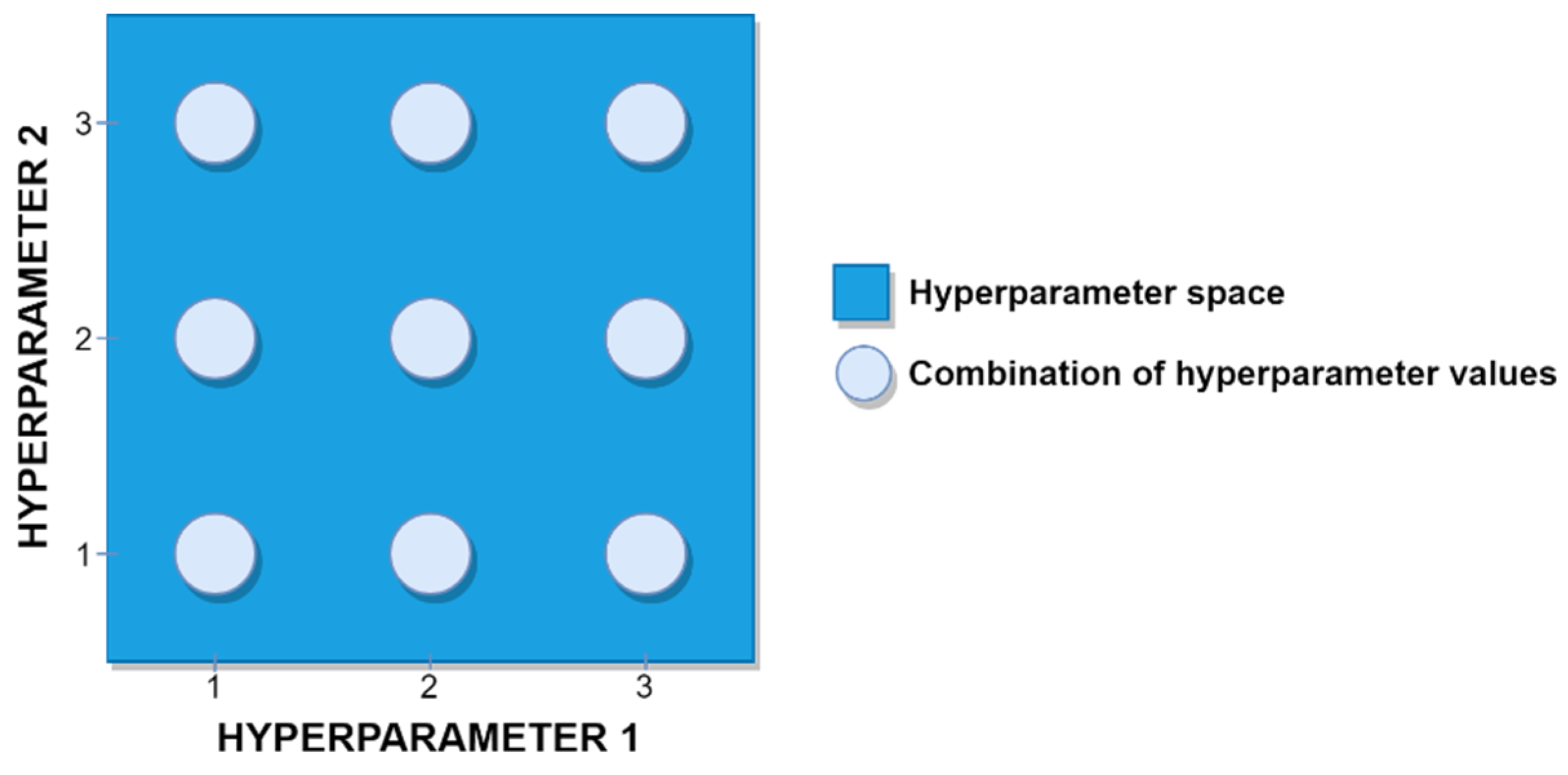
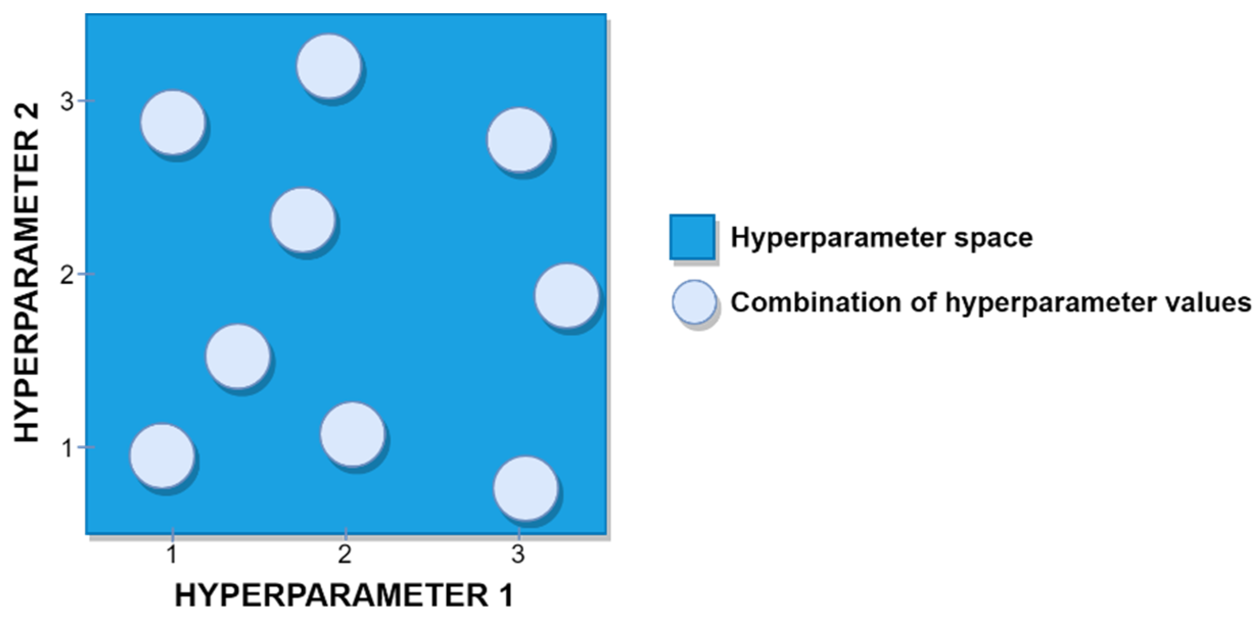
Since evaluating a large number of ML models can be very time-consuming and expensive, many researchers have considered the important problem of how to find an optimal or near-optimal ML model among the set of all possible models as quickly as possible. Unfortunately, many of the hyperparameters involved in ML model training are real-valued, which implies that there is often an infinite number of possible models that theoretically could be evaluated for a particular ML scenario. Recognizing that this situation clearly makes a brute-force model search infeasible, a considerable variety of approaches have been proposed for searching a finite subset of the possible model space. 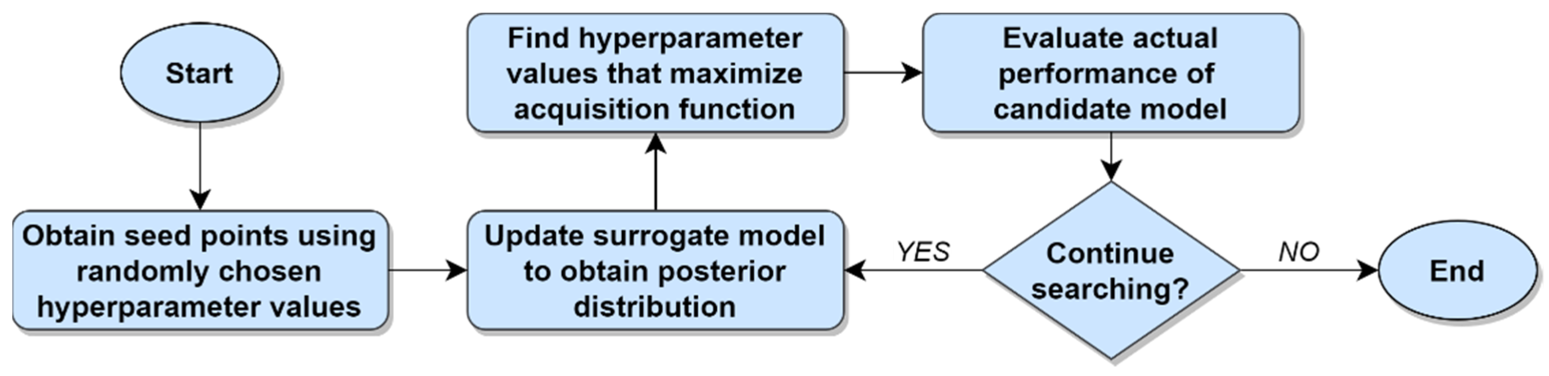The simplest and most common of these methods involve performing a grid search or a random search, with the latter approach serving as a natural baseline for inter-method performance comparisons [5]. 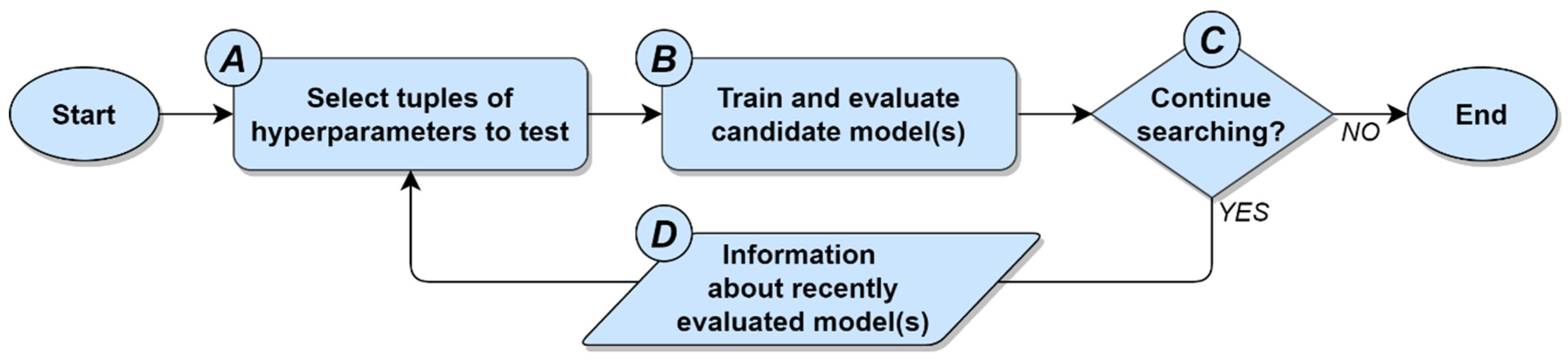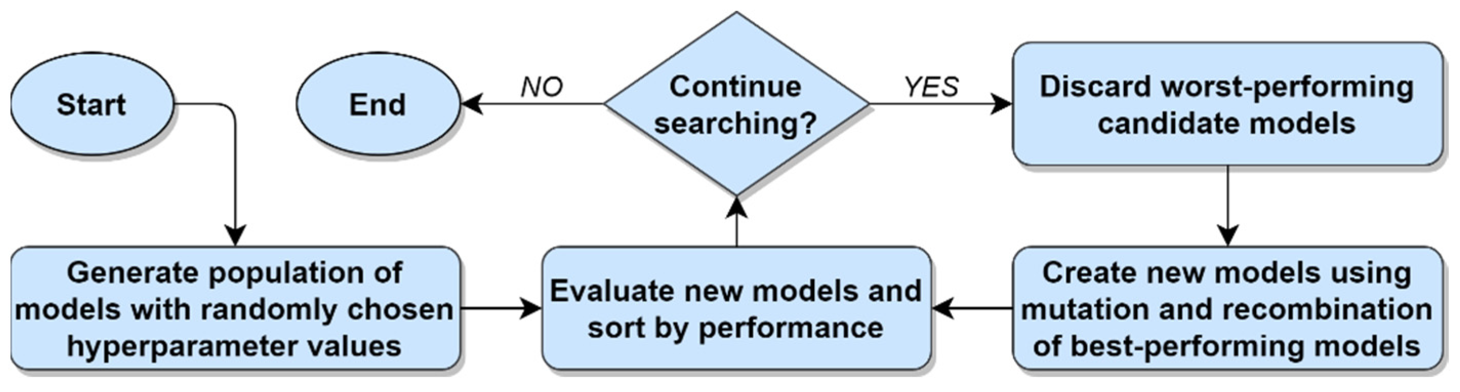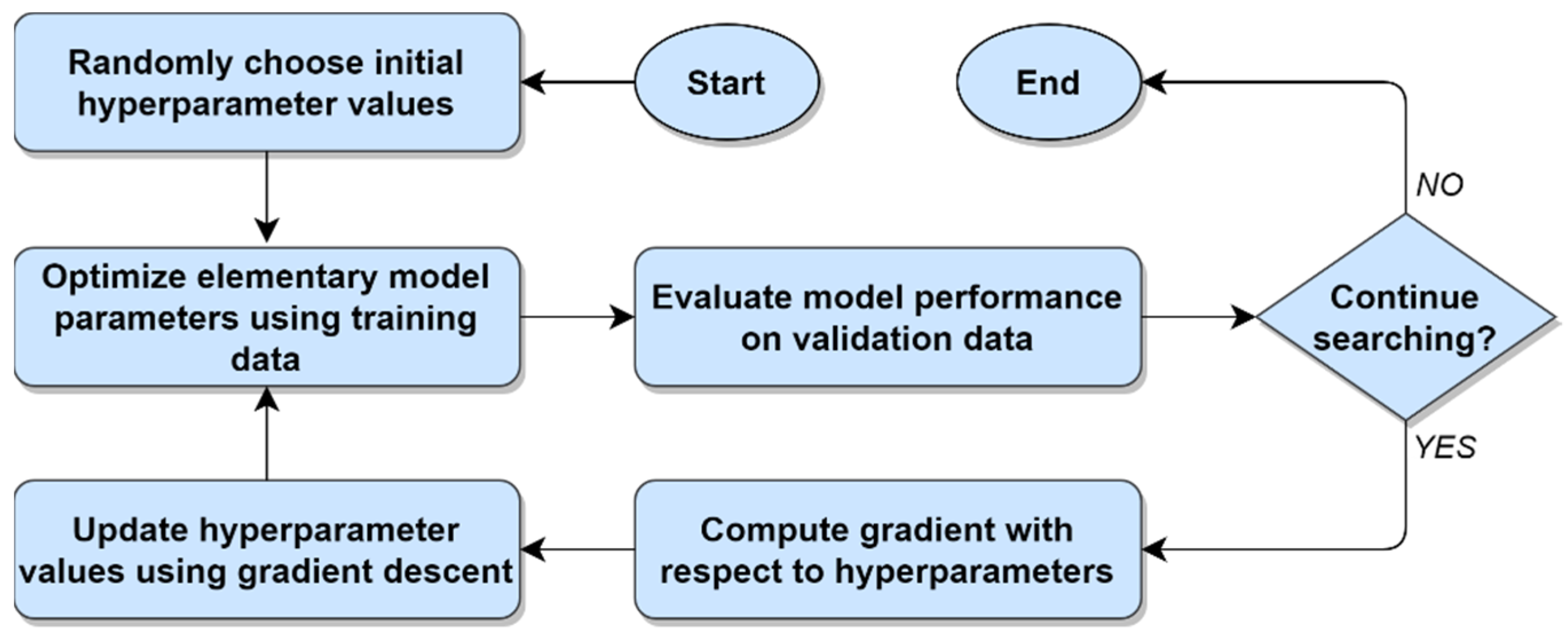Several more sophisticated guided search methods have also been proposed, including Bayesian methods [10], population-based approaches such as evolutionary optimization [11], early stopping methods [12,13], and hypergradient optimization [14,15], etc. Despite the different rules and theories upon which these guided search methods are based, all share a common general strategy: To identify relationships between hyperparameter values and a performance metric, and then use that knowledge to evaluate models located within promising regions of the search space. This general strategy for performing hyperparameter optimization is illustrated in Figure 1 below.

With respect to the general approach to hyperparameter optimization depicted in Figure 1, the factors that distinguish one guided search method from another are (1) variations in how tuples of hyperparameters are selected, (2) which stopping conditions are used, and (3) the information about the relationships between the hyperparameters and the performance metric that is used to guide the search process. Together, these three factors are respectively represented by items A, C, and D in Figure 1. 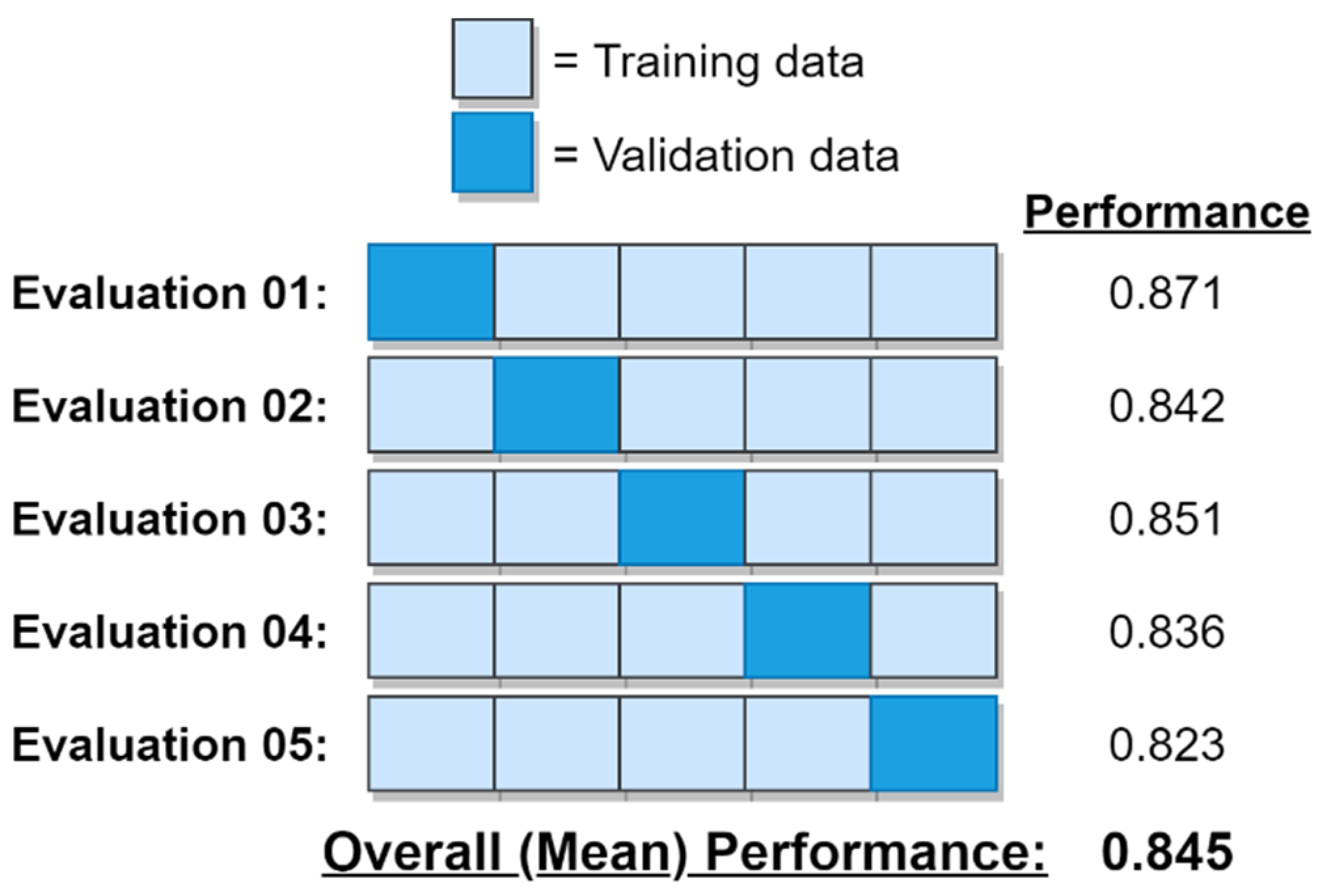What remains, then, is item B, which represents the process of training and evaluating one or more candidate models, with each candidate model corresponding to a tuple of hyperparameter values from item A. Evaluating the performance of each candidate model can be accomplished via any statistically defensible process, regardless of the specific guided search method being used. In practice, the task of evaluating an ML model’s performance is most commonly carried out using k-fold cross validation [16], wherein the data are randomly subdivided into k folds, with each fold being iteratively used as a validation set for a model that has been trained using the remaining folds [17].

In contrast to all extant guided search methods for hyperparameter optimization, the current study takes a completely different approach by considering the ML model training and evaluation process itself as a means of accelerating the search for the best-performing model. Put differently, rather than trying to find promising regions within the hyperparameter space, this study instead focuses on the process of measuring model performance as a way of reducing the time and costs associated with evaluating a large number of candidate ML models. Existing methods of hyperparameter optimization and ML model selection treat cross validation as a simple “black box” process in the sense that they are unconcerned with cross validation itself, and instead are interested only in the output of the cross-validation process. By contrast, the greedy k-fold method proposed herein focuses directly and exclusively on what is happening inside this black box; i.e., the cross validation process itself. With respect to Figure 1, the current study is thus primarily concerned with item B, which, as noted in the discussion above, has been generally overlooked as a means of performing rapid hyperparameter optimization. Given that the ML model performance is most commonly carried out using k-fold cross validation, this paper explicitly seeks to pioneer a new approach to hyperparameter optimization by inquiring into the following general research question:

Research Question: When performing hyperparameter optimization with k-fold cross validation, is it possible to improve the average time required to find the best-performing model by taking a greedy approach to the cross-validation process itself?

The balance of this paper is organized as follows: Section 2 provides a review of the related literature by describing current methods of performing hyperparameter optimization, as well as the standard approach to k-fold cross validation. The greedy k-fold cross validation algorithm that forms the core of the current study is introduced in Section 3, along with a discussion of the algorithm’s properties. Section 3 also introduces an early stopping version of the greedy cross validation algorithm that can be used to quickly identify near-optimal ML models in scenarios that do not involve a computational budget constraint. Section 4 describes two sets of experiments that were undertaken to evaluate the performance of the greedy k-fold method. The first of these evaluates the greedy k-fold method relative to the baseline standard k-fold method, with the experiments comparing the ML model search performance of the greedy and standard methods across a variety of different ML algorithms and real-world datasets. The second set of experiments compares the performance of the early stopping version of the greedy cross validation algorithm against a competing, state-of-the-art early stopping algorithm in terms of both search time and the quality of the selected ML models. The outcomes of the evaluative experiments are presented and discussed in Section 5, with the results indicating that (1) in comparison to the standard k-fold method, greedy k-fold cross validation can vastly reduce the average time required to identify the best-performing ML model among a set of candidate models, and (2) in comparison to the state-of-the-art successive halving algorithm, the early stopping version of the greedy cross validation algorithm generally identifies superior ML models in less time. The paper concludes with Section 6, which provides a brief summary, describes the limitations of the work, and offers a few final remarks about future research directions.

2. Related Work

The primary topic of the current study resides at the intersection of two key concepts from the machine learning literature: (1) Hyperparameter optimization, and (2) k-fold cross validation. Since a familiarity with both of these concepts is a necessary prerequisite for understanding the greedy k-fold cross validation algorithms proposed in Section 3, reviews of both hyperparameter optimization and the standard method of performing k-fold cross validation are provided below.

2.1. Hyperparameter Optimization and Model Selection

When developing ML-based solutions, it is standard practice to evaluate many different ML models with a goal of identifying the model that yields the best possible performance for the problem at hand [18]. The term model as used here refers to a combination of a specific ML algorithm and the specific values that have been chosen for the algorithm’s tunable or definable parameters. These parameters can be structural—for example, the number of hidden layers or the number of nodes per layer in a neural network—or they can be algorithmic parameters that control the learning process, such as the mini-batch size or the learning rate. Collectively, these structural and algorithmic parameters are referred to as the model’s hyperparameters, and the task of searching for the best possible combination of hyperparameter settings for a particular problem is referred to as hyperparameter optimization [5]. Evaluating many combinations of ML algorithms and hyperparameter settings (i.e., evaluating many models) is typically necessary since research has shown that no single ML algorithm or set of hyperparameter settings yields optimal results for all possible datasets or problem domains [19,20]. Indeed, a particular combination of an ML algorithm and a set of hyperparameter settings may perform very well in one scenario while performing very poorly in another scenario. Since every ML model has hyperparameters, and since achieving the best-possible performance is commonly of paramount importance, hyperparameter optimization has become an indispensable step in the broader process of developing an ML-based solution.

2.2. Current Hyperparameter Optimization Methods

Given the necessity of evaluating many candidate ML models via the hyperparameter optimization process, a review of the most common contemporary hyperparameter optimization methods is both appropriate and useful in the context of the current study. As such, the following subsections respectively review the grid search, random search, Bayesian, evolutionary, early stopping, and gradient-based hyperparameter optimization methods.

2.2.1. Grid Search

Grid search has traditionally been one of the most widely used methods of performing hyperparameter optimization among machine learning practitioners [21]. In a grid search, the ML practitioner first specifies a finite set of possible values for each hyperparameter, after which the grid search algorithm performs an exhaustive search by evaluating the Cartesian product of these sets of hyperparameter values [5]. A simple example of a grid search is illustrated in Figure 2 below.

The grid search depicted in Figure 2 includes just two hyperparameters. Since each hyperparameter in the figure has three possible values, a total of nine different combinations of hyperparameter values (i.e., nine different candidate models) would need to be evaluated in this particular scenario in order to find the best-performing model. Different hyperparameters can, of course, have different domains. Whereas some hyperparameters might be categorical (e.g., which regularization method to use), other hyperparameters might be Boolean-valued (e.g., whether or not to learn prior probabilities), integer-valued (e.g., the number of layers in a neural network) or real-valued (e.g., the ML algorithm’s learning rate). In the case of the latter, grid search naturally requires the ML practitioner to discretize real-valued hyperparameters prior to initiating the search process. As with all hyperparameter optimization methods, the ML practitioner must also instruct the grid search algorithm to use a specific performance metric when evaluating a set of candidate models, with overall model performance typically being determined via k-fold cross validation [16]. Finally, it is important to note that grid search suffers from the curse of dimensionality [21]. If, for example, a third hyperparameter with three possible values were added to the simple grid search depicted in Figure 2, the number of candidate models would grow exponentially from $3^2=9$ models to $3^3=27$ models. Since ML algorithms commonly involve a substantial number of hyperparameters with many possible values for each hyperparameter, it can be readily understood how hyperparameter optimization tasks can scale very quickly to hundreds or thousands of candidate models.

2.2.2. Random Search

Rather than iterating over the Cartesian product of all of the sets of hyperparameter values defined by the ML practitioner, a random search proceeds by evaluating ML models whose hyperparameter values have been chosen randomly. As with a grid search, the random search method can be readily applied to discrete, continuous or mixed hyperparameter spaces. For integer-valued or real-valued hyperparameters with unbounded domains, the ML practitioner must typically exercise some judgment by specifying reasonable intervals from which the values for such hyperparameters will be randomly selected. It is common practice when conducting a random search to establish a computational budget for the search process, in which the search for the best-performing model continues until a certain number of models have been evaluated or a certain amount of time has elapsed [5]. A simple example of a random search for an ML scenario involving two real-valued hyperparameters with a computational budget of nine models is illustrated in Figure 3 below.

Random search provides several important advantages when compared to grid search. First, in their highly cited paper, Bergstra and Bengio [21] demonstrated both theoretically and empirically that the random search method is more efficient than the grid search method as a basis for performing hyperparameter optimization. Random search also lends itself very well to parallelization, and supports a more flexible allocation of computational resources than grid search [5]. Furthermore, the distribution from which hyperparameter values are drawn in a random search need not be uniform. Indeed, prior knowledge about the likely usefulness of certain values for a specific hyperparameter within a given ML problem domain can be readily incorporated into a random search by specifying a particular probability distribution from which the random variates for that hyperparameter will be drawn.

Finally, the random search method serves as an excellent baseline against which to compare the performance of other hyperparameter optimization methods. There are several reasons for this. First, the random search method does not make any assumptions about the specific ML problem domain or hyperparameter space in which it is operating. Similarly, the random search method does not make or rely on any assumptions about the specific ML algorithm whose hyperparameters it is attempting to optimize. Lastly, given a sufficient computational budget, a random search will eventually identify a model in the hyperparameter space whose distance from the globally optimal model is within any arbitrarily chosen degree of precision. Since random search has been shown to outperform many sophisticated search algorithms in scenarios involving a fixed computational budget and no prior knowledge of the hyperparameter space, using the performance of a random search as a comparative baseline is critical when evaluating the performance of new metaheuristic search algorithms [22].

2.2.3. Bayesian Optimization

In the context of hyperparameter optimization, Bayesian optimization is an iterative method that relies on Bayes’s Theorem to guide the hyperparameter search process [23]. This method works via a combination of two primary elements: (1) A probabilistic surrogate model, and (2) an acquisition function that is based on the surrogate model [5]. During each iteration, the surrogate model is first updated using the actual observations about the relationship between the hyperparameters and the performance metric that have thus far been obtained, yielding a posterior distribution. The acquisition function is then maximized to identify the most promising tuple of hyperparameter values to evaluate next. A candidate model that uses the most promising tuple of hyperparameter values is then evaluated in the actual search space, with the results being used to update the surrogate model for the next iteration. This process repeats until a stopping condition is met, such as the exhaustion of a computational budget or a sufficiently small difference in candidate model performance from one iteration to the next.

One of the characteristics that makes Bayesian optimization attractive to many ML practitioners is its ability to efficiently produce estimates of how well different models will perform without needing to actually evaluate those models. Using the acquisition function and the surrogate model to estimate the performance of candidate hyperparameter configurations is typically much less computationally expensive than evaluating those hyperparameter configurations directly. The Bayesian optimization algorithm thus capitalizes on what it has learned in order to actually evaluate only those models that it believes to be most promising, while ignoring regions of the search space that it believes to be less promising. The success of this method, of course, naturally depends on how well the surrogate model captures the true relationship between the hyperparameter space and the performance metric. The Bayesian method of performing hyperparameter optimization is illustrated in Figure 4 below.

2.2.4. Evolutionary Optimization

As the name suggests, evolutionary optimization is an iterative method of performing hyperparameter optimization that relies on principles adopted from the biological process of evolution, such as mutation, recombination, adaptation to the environment, and survival of the fittest [24]. The evolutionary optimization process begins by creating a population consisting of a reasonably large number of randomly generated hyperparameter configurations. Next, the performance of each of these members of the population is evaluated in light of the data and the chosen ML algorithm, typically by means of k-fold cross validation. The tuples of hyperparameter values are then ranked according to their observed levels of performance. Next, the worst-performing members of the population are discarded and replaced by new members, with the hyperparameter values for the new members being generated by means of mutation or recombination of the hyperparameter values of the best-performing members of the population. Finally, the performance of each of the newly generated members is evaluated, and the population is re-ranked. These discarding, replacement, and re-ranking tasks are repeated until a stopping condition is met, such as the exhaustion of a computational budget or a sufficiently small difference in the performance of the best-performing candidate model from one iteration to the next. In this way, the population of candidate models steadily evolves towards an optimal solution. As with random search, the evolutionary optimization method lends itself very well to parallelization [25]. The evolutionary method of performing hyperparameter optimization is illustrated in Figure 5 below.

2.2.5. Early Stopping Optimization

Early stopping optimization is an approach to hyperparameter optimization that relies on a strategy of pruning a large number of unpromising hyperparameter configurations as quickly as possible, thus allowing a steadily increasing proportion of the available computational budget to be directed at evaluating more promising hyperparameter configurations in greater detail. Several variants of the early stopping method have been proposed in recent years, notably including successive halving [13,26] (which figures prominently later in this paper), asynchronous successive halving [6], and Hyperband [12]. While each of these early stopping algorithms has distinctive characteristics, the core concepts underlying their operation are consistent. Beginning with a fixed computational budget and a large, randomly generated set of candidate models, the early stopping method first consumes a relatively small proportion of the computational budget by performing a quick, shallow evaluation of each candidate model. Next, the worst-performing models are discarded (i.e., any further consideration of the worst-performing models is stopped early), and a larger proportion of the computational budget is allocated towards evaluating the remaining candidate models in greater detail. This process is then repeated until only a single candidate model remains. Given a fixed computational budget, careful consideration must naturally be given to the tradeoff between the number of candidate models in the initial set and how aggressively the early stopping method prunes poorly performing models during each iteration. A graphical illustration of the early stopping approach to hyperparameter optimization is provided in Figure 6 below.

2.2.6. Hypergradient Optimization

Hypergradient optimization is a general term for the collection of methods that perform hyperparameter optimization by computing a gradient with respect to a ML model’s hyperparameters (i.e., a hypergradient) and then updating the hyperparameter values by using gradient descent [14,15,27,28,29]. Gradient descent and its variants—including stochastic gradient descent, gradient descent with momentum, AdaGrad, Adam, etc.—have been used for several decades as a basis for computing elementary parameter values for a wide variety of ML algorithms [30,31,32]. Following Maclaurin et al. [28], the term elementary parameter is used herein to unambiguously distinguish a machine learning model’s regular parameters from its hyperparameters. Rather than using gradient descent exclusively for the purpose of optimizing a machine learning model’s elementary parameters, however, hypergradient optimization leverages gradient descent as a means of optimizing the model’s hyperparameters, as well.

Hypergradient optimization can be understood as a two-stage or bi-level optimization problem, in which an inner layer of optimization is used to compute values for the ML model’s elementary parameters, while an outer layer of optimization is used to compute values for the model’s hyperparameters [15]. After randomly initializing the ML model’s hyperparameters, hypergradient optimization begins using the training data to perform the initial iteration of optimization on the model’s elementary parameters, typically with a view towards minimizing a cost function. The performance of the model is then evaluated using the validation data. If the candidate model does not satisfy the stopping criterion, then a gradient is next computed, not with respect to the ML model’s elementary parameters, but instead with respect to the model’s vector of hyperparameters. Gradient descent or one of its variants is then applied in order to update the values of the model’s hyperparameters. This two-stage optimization process repeats until the stopping criterion is met. Although hypergradient optimization has shown itself to be highly useful in certain situations, its reliance on gradient descent requires the objective function for the hyperparameters to be differentiable (or at least subdifferentiable). Since many ML algorithms rely on hyperparameters that are not real-valued, this requirement makes the hypergradient approach unsuitable for many hyperparameter optimization problems. The general method of performing hyperparameter optimization via gradient descent is illustrated in Figure 7 below.

2.2.7. Summary of Current Hyperparameter Optimization Methods

Grid search and random search notwithstanding, the conceptual paradigm employed by the other existing methods of ML model selection and hyperparameter optimization described above is to focus on the relationship between the values of the hyperparameters and the values of the metric that is being used to evaluate the performance of each candidate model. More specifically, these hyperparameter optimization methods assume the presence of an underlying but unknown objective function that maps the hyperparameter values for the current ML algorithm to the value of the performance metric. The general goal of such methods, then, is to accumulate information about the nature of the objective function, and then exploit that information to select hyperparameter values that will yield a model whose performance is as close to the global optimum as possible. The greedy method of performing k-fold cross validation described in Section 3 differs from all of these extant guided search methods in that it does not actively compute or choose new hyperparameter values to evaluate as the optimization process unfolds. It also does not treat cross validation as a “black box” process for which the only item of interest is the resulting model performance value. Rather than treating cross validation as a black box, the greedy k-fold method intentionally focuses on the cross-validation process itself, and in so doing demonstrates that the model evaluation task can be exploited as a means of accelerating hyperparameter optimization and ML model selection.

2.3. Standard k-Fold Cross Validation and Model Selection Methods

This subsection provides a brief review of the standard methods of performing k-fold cross validation and ML model selection. Understanding the standard k-fold and model selection processes is important since they serve as the basis of the greedy k-fold cross validation algorithm described in Section 3.

2.3.1. Standard k-Fold Cross Validation

Broadly, k-fold cross validation is a technique for judging how well a model will generalize to scenarios involving novel data that were not considered or “seen” when the model was being trained [33,34]. In the context of machine learning, k-fold cross validation has become the primary method used by ML practitioners when evaluating candidate models [16], not only due to the method’s utility as an estimator of generalization performance, but also due to its ability to reveal problems with selection bias and overfitting [35]. The standard k-fold process involves splitting the data into k subsets (called folds), with each fold being iteratively used as a validation set for a candidate model that has been trained using the data from the remaining folds [17]. Each fold contains an equal or approximately equal number of cases, with fold membership typically being assigned randomly. If the dataset is relatively small, stratified random sampling may also be used in order to ensure that the target variable is approximately identically distributed in each fold [36]. After splitting the data into k folds, the candidate model is next subjected to an iterative evaluation process. During each evaluative iteration, k-1 of the folds are used to train the candidate model, with the model’s performance being measured using the remaining fold. This process is repeated until each fold has been used exactly once as a validation set, yielding a total of k iterations of training and validation for each candidate model. Finally, the model’s overall performance θ is estimated as the mean of the performance values obtained from each iteration, as shown in Equation (1). The standard method of performing k-fold cross validation is illustrated in Figure 8.

$$\theta =\frac{1}{k}{{\displaystyle \sum }}_{i=1}^k{\theta }_i$$

(1)

2.3.2. Model Selection

Given a specific problem scenario and machine learning algorithm, the most widely used strategy for identifying and selecting the best-performing ML model is to conduct hyperparameter optimization using k-fold cross validation [35,37]. The set of candidate models to be evaluated may be defined in advance (e.g., when using a grid search, random search or early stopping search) or may be defined dynamically as the model search process unfolds (e.g., when using the Bayesian, evolutionary or hypergradient guided search methods described previously). After evaluating as many models as possible given the constraints of the computational budget (or when a stopping criterion is met in the absence of a computational budget), the candidate model with the most desirable overall performance characteristics is chosen as the final model. A wide variety of performance metrics are feasible for the model selection process (e.g., best classification accuracy, lowest mean squared error, etc.), with the choice of metric being situationally dependent on the specific ML method and the specific task at hand. The standard approach to selecting an optimal ML model via k-fold cross validation for a scenario involving a predefined set of candidate models is described in Algorithm 1 below.

Algorithm 1. Standard approach to ML model selection via k-fold cross validation.

Input: M (set of candidate models), k (number of folds), D (dataset), b (computational budget) Output: Best-performing, fully evaluated model split D into k folds, s.t. D = {d1, d2, …, dk} η ← 0   (number of fold evaluations completed) while η < b do   (while the computational budget is not exhausted)    m = next model in M    for j = 1 to k do      train m using all folds di ∈ D where i ≠ j      evaluate performance of m using fold dj      Ρm ← mean performance of m for folds {d1, …, dj}      η ← η + 1      if η ≥ b then break   (if the computational budget is exhausted)    end for end while return best, fully evaluated m ∈ M, per Ρ

Note that the standard k-fold algorithm can be readily modified to support any of the guided search methods described previously. This can be accomplished by eliminating the assumption that the set of candidate models is known in advance, and instead implementing a framework in which the next model to be evaluated is determined at runtime based on what has been learned about the relationship between the values of the hyperparameters and the performance metric. A graphical representation of the standard k-fold cross validation algorithm being used to select the best-performing candidate model is shown in Figure 9 below.

As shown in the figure above, the combination of n candidate models and k evaluative iterations can be thought of as a table, with each column representing one of the k evaluative iterations and each row representing a candidate model. The overall progress that has been made towards completing the evaluation of each candidate model is indicated by the color of the table cells, with dark-colored cells indicating that the evaluative iteration has been completed for the corresponding fold and model. Evaluation of candidate models thus proceeds one fold at a time, from left to right, top to bottom until the computational budget has been exhausted, at which time the fully evaluated candidate model with the best overall performance is chosen as the final model. Using this conceptual framework, it is convenient to discuss the total amount of work involved in the ML model selection process in terms of the number of folds evaluated, where a “fold evaluation” refers to a fold being used to validate a candidate model that has been trained with the remaining folds. The maximum number of folds that could possibly be evaluated in the ML model selection process is thus $nk$, with reasonable values for a computational budget $b$ falling in the interval $k\le b\le nk$.

3. Greedy k-Fold Cross Validation

The two versions of the greedy k-fold cross validation algorithm proposed in this section take a completely different approach to hyperparameter optimization than any of the guided search methods described previously. Specifically, whereas these existing methods seek to accelerate the ML model search process by identifying and searching promising areas within the hyperparameter space, the general approach of the greedy k-fold method is to focus on the k-fold cross-validation process itself as a means of achieving rapid hyperparameter optimization and model selection. At a fundamental level, the greedy k-fold cross validation method proposed here differs from the standard k-fold cross validation process in just one important way. In the standard approach, all of the folds for a given ML model are considered as validation sets in sequential order, one after another, thus allowing the overall performance of the model to be computed before the algorithm moves on to the next candidate model (i.e., within-model evaluation). By contrast, greedy k-fold cross validation considers a sequence of folds that originate from different ML models, with the specific model and validation fold to use next being greedily chosen at runtime. Put differently, the standard approach to k-fold cross validation can be thought of as relying on a sequence of within-model fold evaluations, while the greedy approach to k-fold cross validation can be thought of as relying on a sequence of between-model fold evaluations.

The greedy k-fold cross validation algorithm begins by obtaining a partial performance estimate for each candidate model using just the first fold as a validation set, after having trained the model using the remaining folds. The model with the best initial performance is then identified, after which the second fold for that model is used as a validation set (with the remaining folds naturally being used as the training set). The performance estimate for the model is then updated to reflect the mean performance observed after having tested the model using the first two folds as validation sets. The model with the best mean performance at that moment is then identified, after which its next available fold is used as a validation set and the model’s mean performance is updated. This process repeats until either the computational budget has been exhausted or an early stopping criterion has been met, at which time the algorithm returns the best, fully evaluated model. The process of selecting an optimal ML model using greedy k-fold cross validation when operating under the constraint of a computational budget is described in Algorithm 2 below.

Algorithm 2. ML model selection using greedy k-fold cross validation with a computational budget.

Input: M (set of candidate models), k (number of folds), D (dataset), b (computational budget) Output: Best-performing, fully evaluated model split D into k folds, s.t. D = {d1, d2, …, dk} for each m ∈ M do    train m using folds {d2, …, dk}    Ρm ← performance of m evaluated using fold d1    Fm ← 1   (number of folds evaluated for m) end for η ← #M   (set number of completed fold evaluations to cardinality of M) while η < b do (while the computational budget is not exhausted)    m* = best incompletely evaluated m ∈ M   (given the current mean performance for each m, per Ρ)    Fm* ← Fm* + 1    train m* using all folds di ∈ D where i ≠ Fm*    evaluate performance of m* using fold dFm*    Ρm* ← mean performance of m* for folds {d1, …, dFm*}    η ← η + 1 end while return best, fully evaluated m ∈ M, per Ρ

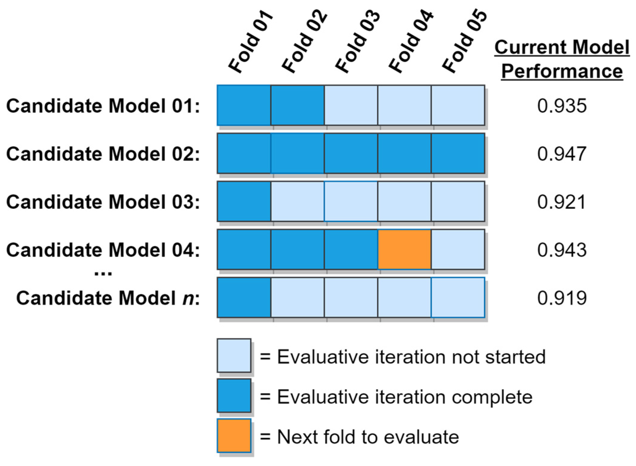
As indicated in the while loop, the greedy k-fold cross validation algorithm behaves greedily by always pursuing the most promising available option, with the extent to which an option is promising being determined by the current mean performance of its corresponding model. Put differently, the next fold that the greedy algorithm will evaluate will always originate from the best incompletely evaluated model, as determined by each candidate model’s current mean performance. 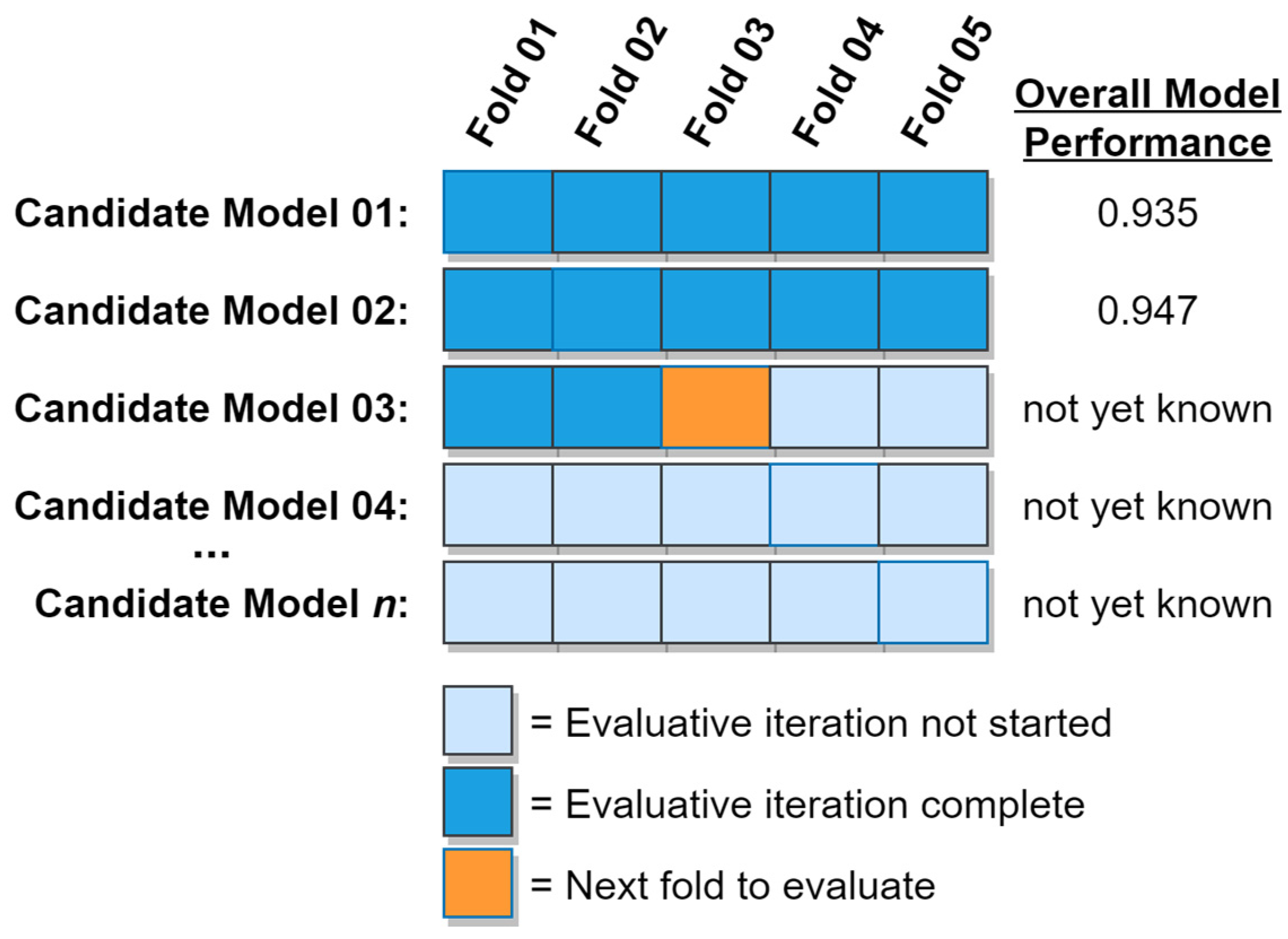In this way, the greedy k-fold cross validation algorithm focuses its early efforts on the most promising candidate models. As time passes and the most promising models become fully evaluated, the algorithm will steadily evaluate folds from less and less promising models, but will never waver from the principle of greedily pursuing the most promising of its available options on each iteration. In the presence of a computational budget constraint, this behavior thus increases the probability of an optimal or near-optimal model being identified before the computational budget is exhausted. If instead an early stopping criterion based on model performance is being used, this behavior helps ensure that the early stopping criterion will be met as quickly as possible, thus accelerating the overall model search process. A graphical example of the greedy k-fold cross validation algorithm is shown in Figure 10. In the figure, Candidate Model 02 has already been fully evaluated, while evaluation of the remaining models is still in progress.

Since hyperparameter optimization and ML model selection tasks do not always occur under the constraint of a computational budget, a variation of the greedy k-fold cross validation method in which a simple early stopping criterion has been implemented is described in Algorithm 3 below. This criterion allows the greedy cross validation algorithm to decide whether to continue searching or to stop the search process early based on the data, rather than relying on a predefined computational budget constraint. In this variant of the greedy cross validation algorithm, an early stopping percentage (ε) is provided as an input parameter. The product of ε and the number of candidate models is run through a standard ceiling function to yield an early stopping threshold. Every time a candidate model becomes fully evaluated, that model’s overall performance is compared to the performance of the currently known, fully evaluated, best-performing model. If the newly completed model is found to be inferior to the currently known best model, then an inferior model counter is incremented. Whenever the value of the inferior model counter exceeds the early stopping threshold, the search is stopped immediately and the currently known, fully evaluated, best-performing model is returned. If, however, a newly completed candidate model is found to be superior to the currently known best model, then the newly completed model replaces the previous best-performing model, and the inferior model counter is reset to zero. In this way, the algorithm will continue searching as long as it continues to find better and better models. As soon as this steady improvement falters (as signaled by a sufficiently large succession of inferior models), the search process is terminated.

Algorithm 3. ML model selection using greedy k-fold cross validation with early stopping.

Input: M (set of candidate models), k (number of folds), D (dataset), ε (early stopping percentage) Output: Best-performing, fully evaluated model split D into k folds, s.t. D = {d1, d2, …, dk} for each m ∈ M do    train m using folds {d2, …, dk}    Ρm ← performance of m evaluated using fold d1    Fm ← 1 (number of folds evaluated for m) end for η ← #M   (set number of completed fold evaluations to cardinality of M) ι ← 0   (initialize inferior model counter) while η < #M∙k do   (while there are more folds to be evaluated)    m* = best incompletely evaluated m ∈ M   (given the current mean performance of each m, per Ρ)    Fm* ← Fm* + 1    train m* using all folds di ∈ D where i ≠ Fm*    evaluate performance of m* using fold dFm*    Ρm* ← mean performance of m* for folds {d1, …, dFm*}    η ← η + 1    if Fm* = k then   (if all folds for m* have been evaluated)      if Pm* is the best performance thus far observed then       ι ← 0   (reset inferior model counter)      else   (if m* is inferior to the currently known, fully evaluated, best-performing model)       ι ← ι + 1        if $\iota >\lceil \#M·\epsilon \rceil$ then (if the inferior model counter exceeds the early stopping threshold)          break   (exit the loop immediately)        end if      end if    end if end while return best, fully evaluated m ∈ M, per Ρ

4. Materials and Methods

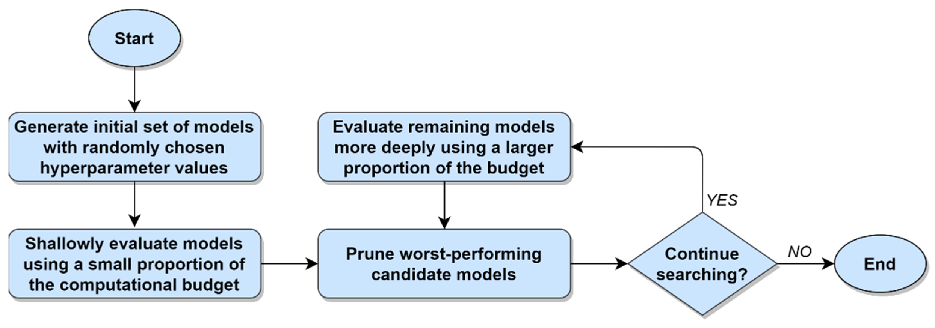
Having presented two variants of the greedy k-fold cross validation algorithm, this section describes two sets of evaluative experiments that were undertaken to assess the performance of each of those variants. The first group of experiments addressed scenarios involving a computational budget by comparing the performance of Algorithm 2 to that of the standard k-fold method. The second group of experiments addressed scenarios without a computational budget by comparing the performance of Algorithm 3 to a leading early stopping method – the successive halving algorithm [12,13]. To rigorously evaluate each variant of the greedy k-fold method, its performance was compared to its respective competing method (either standard k-fold or successive halving) under many experimentally manipulated conditions, including using a variety of different ML algorithms, a variety of real-world datasets, and varying values of the number of folds (k) and the number of candidate models (n). Before describing these experiments, however, it is necessary to define the way in which the performance of the various methods was measured in the experiments.

4.1. Performance Metrics

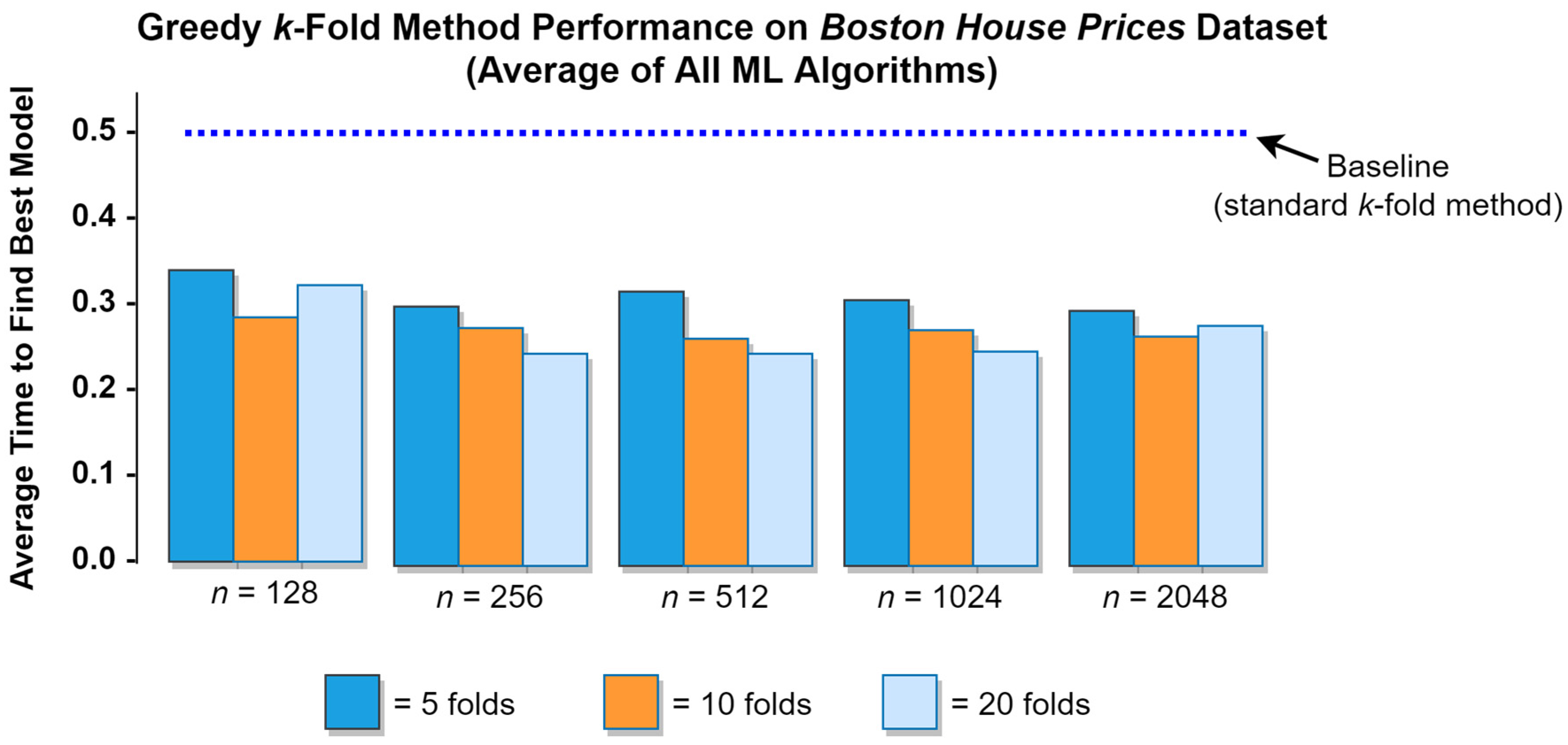
Beginning with the first group of experiments—in which the greedy k-fold cross validation method was compared to the standard k-fold cross validation method—recall from the earlier discussion that for a hyperparameter space containing n models that are tested with cross validation using k folds, the total number of fold evaluations is nk. For a set of n candidate models, then, the performance of each method in the first group of experiments was measured by the average search time required to find the best-performing model in the set, with search time being calculated as the ratio of the total number of fold evaluations that were required to find the best-performing model relative to the total number of nk possible fold evaluations. This is a very convenient measure of search time since it naturally yields an interval that ranges from 0.0 to 1.0, thus allowing straightforward performance comparisons to be made across experimental conditions. Given the search time metric described above, it can be readily calculated that the time required to fully evaluate each candidate model is $k/nk=1/n$. The maximum theoretical time required to find the optimal model using the standard k-fold method is thus $nk/nk=1.0$, while the minimum search time for the standard method is $1/n$. Since the standard k-fold method essentially employs a linear search strategy, the average theoretical search time for the standard method is $1/nk·nk/2=1/2$. On average, then, the standard k-fold cross validation method can be expected to find the optimal model after having fully evaluated 50% of the candidate models. While the maximum theoretical search time for the greedy k-fold method is also 1.0, the minimum time for the greedy method to find the optimal model is $\left(n+k-1\right) / nk$. The average theoretical search time for the greedy k-fold method will depend on the distributional properties of the training dataset and will hence vary from one ML scenario to the next.

For the second group of experiments—which compared the early stopping version of the greedy k-fold cross validation method to the successive halving method—a different set of performance metrics was required. The reason for this is that, by definition, early stopping algorithms stop the model search process early, and hence do not completely evaluate every model in the set of candidate models. As such, we can never be entirely certain that the final model chosen by an early stopping method is truly the best-performing model in the set of candidate models. Furthermore, it would be inequitable to quantify the search time for the greedy early stopping method and the successive halving method using the same metric from the first group of experiments, since the two algorithms evaluate neither the same number of folds nor folds consisting of the same number of cases. With these considerations in mind, two performance metrics were designed for the second set of experiments that compare each of the competing algorithms to a common baseline. Specifically, for each comparison of the greedy and successive halving early stopping methods, the common set of candidate models provided as input to each method was first fully evaluated using the standard k-fold method described in Algorithm 1. For any set of candidate models used in the second group of experiments, this approach thus provided a true performance ranking for each model in the set, as well as measurement of the total wall-clock time required by the standard k-fold method to conduct a complete search of every candidate model in the set. With this information available for each experiment, it was possible to compute two equitable metrics for comparing the greedy and successive halving early stopping methods, the first of which addressed the quality of the final model selected by each algorithm, and the second of which addressed the wall-clock time required by each algorithm to complete the model search process. In the case of the former, the quality of the final model selected by each algorithm was measured as the rank-based percentile of the chosen model relative to the true best-performing model in the set of candidate models. If, for example, an early stopping algorithm was given a set of n = 100 candidate models to consider and it ultimately selected the second-best model in the set, then the quality of the algorithm’s choice would be scored as (100−1)/100 = 0.99, indicating that only 1% of the other models in the set were superior to the chosen model. In the case of the latter, the speed of each early stopping algorithm was computed as the ratio of the wall-clock time required by the algorithm to complete the model search relative to the wall-clock time required by the standard k-fold method to perform an exhaustive search on the same set of candidate models. If, for example, an early stopping algorithm required 30 s to complete the search process while a comparable exhaustive search required 100 s, then the speed of the early stopping method for that experiment would be scored as 30/100 = 0.30, indicating that the early stopping method needed only 30% of the time required by the standard k-fold method to complete the model search.

4.2. ML Algorithms and Datasets

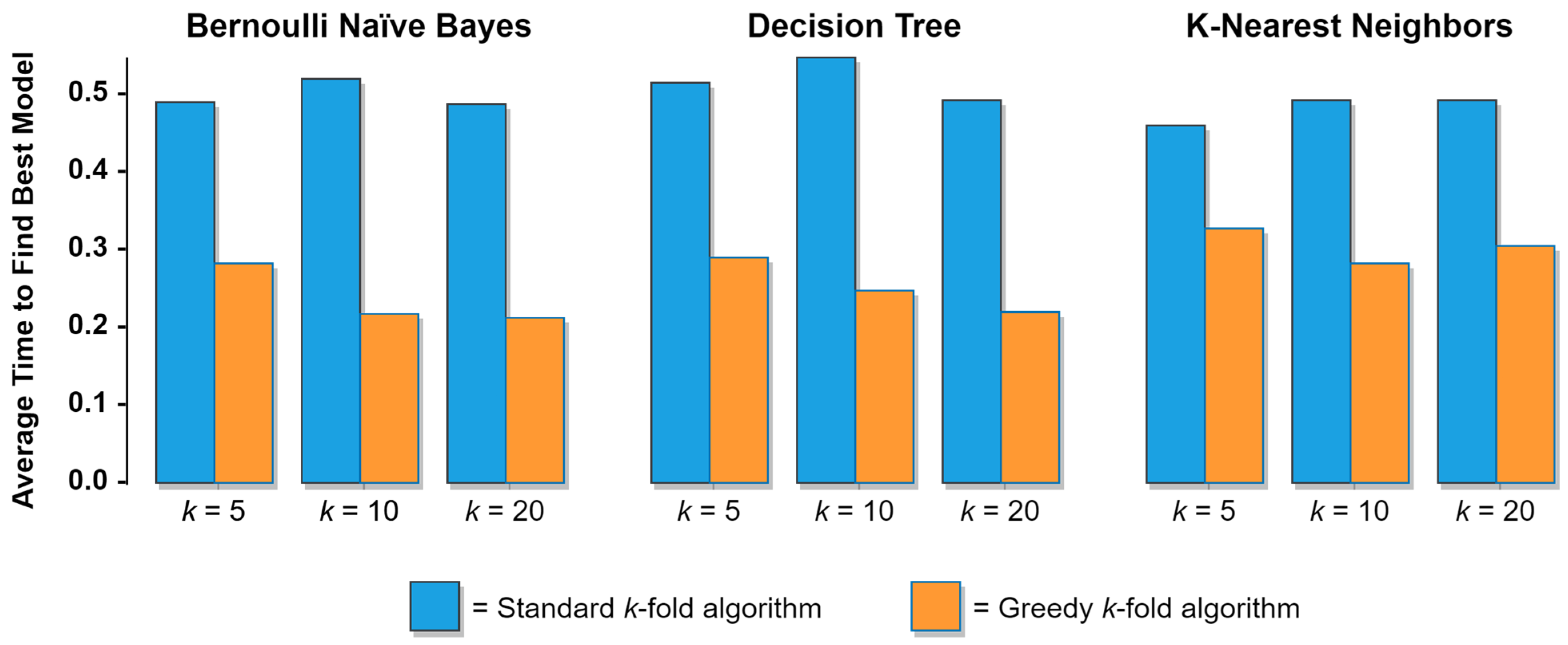
As noted previously, a variety of ML algorithms and real-world datasets were used in the experiments to compare the performance of the greedy k-fold cross validation method to the standard (baseline) k-fold cross validation and successive halving methods. These algorithms included the Bernoulli Naïve Bayes, Decision Tree, and K-Nearest Neighbors (KNN) classifiers, each of which was chosen due to its distinct approach to performing the classification task. All of the ML algorithms used in the experiments are open-source and freely available via the Python scikit-learn library [38]. The three datasets used in the experiments are all well-known among ML practitioners and included the Wisconsin Diagnostic Breast Cancer dataset (569 cases, 30 features, 2 classes), the Boston Home Prices dataset (506 cases, 13 features, 4 classes—discretized using a quartile split), and the Optical Recognition of Handwritten Digits dataset (1797 cases, 64 features, 10 classes). These three datasets were chosen since they varied widely in terms of their numbers of cases, features, and classes, and since they are all freely available as part of the scikit-learn library [38], thus helping ensure that the results of the experiments can be easily replicated.

4.3. ML Models and Folds

For each combination of ML classifier and dataset, n different candidate models were evaluated in each experiment. The set of values used in the experiments for n was derived from a geometric sequence with a common factor of two: $f\left(x\right)=2^x$. For the first group of experiments (which extensively compared the greedy and standard k-fold cross validation methods), $x\in \left\{7, 8, \dots , 11\right\}$, yielding $n\in \left\{128, 256, 512, 1024, 2048\right\}$. For the second group of experiments (which compared the greedy and successive halving early stopping methods), $x\in \left\{ 8, 9, 10\right\}$, yielding a narrower $n\in \left\{256, 512, 1024\right\}$. A variety of values of k were also used for the first group of experiments, with each cross-validation method being evaluated with $k\in \left\{5, 10, 20\right\}$ folds. These values of k were chosen based on their common usage in applied ML projects. For the second group of experiments comparing the performance of the greedy and successive halving early stopping methods, each experiment relied on k = 10 folds. The candidate models that were evaluated in the experiments varied according to the values of their hyperparameters, with the hyperparameter settings for each model being chosen randomly in accordance with Bergstra and Bengio [21] using the same ranges of possible values for each hyperparameter that were used by Olsen et al. [19].

4.4. Experiment Procedure

For each combination of ML classifier, dataset, and n, the same set of candidate models was used to evaluate the competing methods in each experiment. This approach was adopted to ensure that any differences in inter-method performance could not be attributed to variation in hyperparameter settings among the n available models. For the first group of experiments, all n candidate models were fully evaluated using the standard and greedy cross validation methods during each experiment, with the completion time and value of the performance metric being recorded for each model and method. After all of the candidate models had been evaluated, the best-performing model and its corresponding evaluation completion times were identified for each cross-validation method. For the second group of experiments, all n candidate models were first fully evaluated by the standard k-fold cross validation method for each experiment in order to establish a baseline model search time and to identify the true performance rank for each model. The same candidate models were then provided to the greedy and successive halving early stopping methods, with the expectation that each method would partially evaluate the set of candidate models according to the tenets of its respective algorithm. For the current study, a value of 0.02 (or 2%) was used as the ε (early stopping percentage) parameter for the greedy early stopping algorithm. After completing the model search process, the elapsed wall-clock time and the true performance rank of each method’s chosen model were used to calculate the comparative search time and model quality metrics for that experiment, as described previously in Section 4.1.

Finally, a total of 30 iterations of each experiment were carried out in the manner described immediately above in order to ensure that the resulting distributions of the performance metrics would be approximately Gaussian, per the central limit theorem [39]. The performance of the greedy cross validation method could then be compared to the standard method (for the first set of experiments) and to the successive halving method (for the second set of experiments) in each of the experimental conditions by means of a Welch’s t-test. Welch’s t-tests were used in these comparisons since there was no reason to expect that the variances of the distributions of the performance metrics for the various methods would be equal, and Welch’s t-tests allow for unequal variances [40]. The results of the experiments are reported and discussed in the following section.

5. Results and Discussion

5.1. Experiments Comparing the Greedy and Standard k-Fold Cross Validation Methods

The average search time required by the greedy and standard k-fold cross validation methods to find the optimal model using the different ML algorithms, datasets, and values of k is provided in

Table 1. Average search time to find the optimal model.

Dataset	Algorithm	Greedy k-Fold Method			Standard k-Fold Method
		k = 5	k = 10	k = 20	k = 5	k = 10	k = 20
Boston Home Prices	Bernoulli Naïve Bayes	0.342 ***	0.299 ***	0.301 ***	0.495	0.496	0.496
	Decision Tree	0.280 ***	0.231 ***	0.229 ***	0.522	0.524	0.514
	K-Nearest Neighbors	0.320 ***	0.291 ***	0.278 ***	0.501	0.488	0.489
Wisconsin Diagnostic Breast Cancer	Bernoulli Naïve Bayes	0.282 ***	0.217 ***	0.212 ***	0.491	0.521	0.488
	Decision Tree	0.291 ***	0.248 ***	0.219 ***	0.516	0.547	0.492
	K-Nearest Neighbors	0.328 ***	0.283 ***	0.306 ***	0.459	0.493	0.492
Optical Recognition of Handwritten Digits	Bernoulli Naïve Bayes	0.236 ***	0.164 ***	0.146 ***	0.523	0.515	0.468
	Decision Tree	0.231 ***	0.148 ***	0.113 ***	0.494	0.440	0.526
	K-Nearest Neighbors	0.270 ***	0.193 ***	0.191 ***	0.504	0.482	0.530

*** p < 0.001 for a Welch’s t-test comparing the performance of the greedy method to the standard method.

below, with the results in the table being computed using all possible values of n. Probability values reported in Table 1 were derived from two-tailed Welch’s t-tests for which the performance of the greedy method was compared to the performance of the standard method in corresponding experimental conditions. As shown in the table, in terms of its ability to quickly identify the optimal model, the greedy k-fold method statistically outperformed the standard k-fold method at the p < 0.001 level in every combination of dataset, ML algorithm, and value of k used in the experiments. These results provide strong statistical evidence for the superiority of the greedy k-fold method over the standard k-fold method in identifying optimal or near-optimal ML models when operating under the constraints of a computational budget.

Having observed strong statistical evidence for the superiority of the greedy k-fold method, it is reasonable to next inquire into the relative magnitude of that superiority. Among the 27 unique combinations of datasets, ML algorithms, and values of k reported in Table 1, the overall mean search time for the greedy method was 0.246 (std dev = 0.059), while the overall mean search time for the standard method was 0.500 (std dev = 0.023). This suggests that among the datasets and ML algorithms used in the experiments, the greedy method on average identified the optimal model among the set of n candidate models after completing 24.6% of the possible fold evaluations, while the standard method on average identified the optimal model after completing 50.0% of the possible fold evaluations. Note that this latter outcome conforms precisely with the theoretically expected average for the standard method described in Section 4.1. Put differently, the greedy k-fold cross validation method identified the best-performing ML model among the set of candidate models more than twice as quickly on average than the standard k-fold method. As an illustrative example of this major difference in performance, Figure 11 below depicts the average search time of the greedy vs. standard k-fold methods using the three different ML algorithms on the Wisconsin Diagnostic Breast Cancer dataset.

The results presented in Table 1 and Figure 11 reflect the comparative performance of the standard and greedy k-fold methods across a variety of datasets, ML algorithms, and values of k. Those results, however, were computed for all of the possible values of n that were used in the first group of experiments. It is, of course, possible to gain more detailed insights by disaggregating these results and considering how various values of n impact the comparative performance of the standard and greedy k-fold methods. While the limitations of print media make it infeasible to visualize the comparative performance of these two different cross validation methods for all 135 unique combinations of datasets, ML algorithms, values of k, and values of n used in the first group of experiments, a representative example is provided in Figure 12 below. This figure shows how the greedy k-fold method performed against the standard (baseline) k-fold method for varying numbers of n candidate models on the Boston House Prices dataset at values of $k\in \left\{5, 10, 20\right\}$.

Regardless of the dataset, ML algorithm, number of folds or number of candidate models, the greedy k-fold method was observed to consistently outperform the standard k-fold method on average in all of the 135 comparisons that constituted the first set of experiments. In the absence of counterevidence, these observations provide support for the notion that the greedy k-fold algorithm is generally superior to the standard k-fold algorithm in quickly identifying optimal ML models, regardless of the dataset, ML algorithm, number of folds or number of candidate models. Since the data suggest that the greedy method is, on average, approximately twice as efficient as the standard method in terms of its ability to quickly locate top-performing ML models, it is recommended that the greedy method be given serious consideration in any machine learning hyperparameter tuning/model selection scenario involving a computational budget constraint.

5.2. Experiments Comparing the Greedy Early Stopping and Successive Halving Methods

The second set of experiments conducted in this study compared the performance of the greedy early stopping method described in Algorithm 3 against the performance of the state-of-the-art successive halving method, both in terms of the average quality of the final ML models selected by each method and in terms of each method’s average model search time. The average quality of the final ML model selected by the greedy and successive halving early stopping methods using different combinations of ML algorithms, datasets, and values of n is provided in

Table 2. ML model selection performance for the greedy early stopping and successive halving methods.

Dataset	Algorithm	Greedy Early Stopping Method			Successive Halving Method
		n = 256	n = 512	n = 1024	n = 256	n = 512	n = 1024
Boston Home Prices	Bernoulli Naïve Bayes	0.959 ***	0.986 ***	0.970 ***	0.777	0.791	0.820
	Decision Tree	0.994 ***	0.997 ***	0.999 ***	0.641	0.596	0.631
	K-Nearest Neighbors	0.923 ***	0.944 ***	0.937 ***	0.632	0.698	0.662
Wisconsin Diagnostic Breast Cancer	Bernoulli Naïve Bayes	0.981 ***	0.991 ***	0.989 ***	0.815	0.859	0.900
	Decision Tree	0.997 ***	0.998 ***	0.999 ***	0.676	0.621	0.674
	K-Nearest Neighbors	0.948 ***	0.957 ***	0.934 ***	0.695	0.587	0.477
Optical Recognition of Handwritten Digits	Bernoulli Naïve Bayes	0.996 **	0.999 ***	1.000 ***	0.982	0.979	0.971
	Decision Tree	0.998 ***	0.998 ***	1.000 ***	0.890	0.860	0.859
	K-Nearest Neighbors	0.982 ***	0.974 ***	0.980 ***	0.851	0.815	0.840

** p < 0.01, *** p < 0.001 for a Welch’s t-test comparing the quality of the final ML models selected by the greedy early stopping method and the successive halving method in corresponding experimental conditions.

below. As noted in Section 4.1, these results reflect the average rank-based percentile of a chosen model relative to the true optimal model in the set of candidate models used in an experiment. As with Table 1, probability values reported in Table 2 were derived from two-tailed Welch’s t-tests for which the performance of the greedy early stopping method was compared to the performance of the successive halving method in corresponding experimental conditions.

As shown in the table, in terms of its ability to select high-performing models, the greedy early stopping method statistically outperformed the state-of-the-art successive halving method in every combination of dataset, ML algorithm, and value of n used in the early stopping experiments. From an interpretive perspective, this means that the greedy early stopping method was, on average, able to select final ML models that performed better than the final ML models selected by the successive halving method in every one of the 27 head-to-head experiments conducted in this study. These results provide strong statistical evidence for the superiority of the greedy early stopping method over the successive halving method in identifying optimal or near-optimal ML models.

While establishing the ability of the greedy early stopping algorithm to select higher-quality ML models than the successive halving algorithm is certainly necessary, it is not by itself sufficient to establish the overall superiority of the greedy method. Indeed, the primary goal of any hyperparameter optimization and ML model selection algorithm is not just to select optimal or near-optimal models, but also to do so as quickly as possible. For this reason, it is necessary to compare the performance of the greedy early stopping method to that of the successive halving method in terms of the wall-clock time required by each approach to complete the ML model search process. To this end, the average wall-clock time required by the greedy and successive halving early stopping methods to complete the ML model search process under conditions involving different combinations of ML algorithms, datasets, and values of n is provided in

Table 3. ML model search times for the greedy early stopping and successive halving methods.

Dataset	Algorithm	Greedy Early Stopping Method			Successive Halving Method
		n = 256	n = 512	n = 1024	n = 256	n = 512	n = 1024
Boston Home Prices	Bernoulli Naïve Bayes	0.229 ***	0.235 ***	0.199 ***	0.759	0.716	0.675
	Decision Tree	0.204 ***	0.193 ***	0.191 ***	0.421	0.388	0.361
	K-Nearest Neighbors	0.210 ***	0.209 ***	0.217 ***	0.438	0.419	0.405
Wisconsin Diagnostic Breast Cancer	Bernoulli Naïve Bayes	0.219 ***	0.204 ***	0.204 ***	0.688	0.652	0.598
	Decision Tree	0.242 ***	0.224 ***	0.207 ***	0.290	0.272	0.252
	K-Nearest Neighbors	0.248 *	0.229 *	0.235	0.301	0.288	0.275
Optical Recognition of Handwritten Digits	Bernoulli Naïve Bayes	0.178 ***	0.179 ***	0.184 ***	0.337	0.311	0.289
	Decision Tree	0.219	0.198	0.211	0.166 ***	0.144 ***	0.127 ***
	K-Nearest Neighbors	0.221	0.195	0.219	0.052 ***	0.044 ***	0.041 ***

* p < 0.05, *** p < 0.001 for a Welch’s t-test comparing the wall-clock time required by the greedy early stopping and successive halving methods to complete the ML model search process in corresponding experimental conditions.

below. As noted in Section 4.1, these results reflect the average wall-clock time required to complete the model search process relative to the total wall-clock time required by the standard k-fold method to perform a full, exhaustive search of the same set of candidate models used in an experiment. As with the previous table, probability values reported in Table 3 were derived from two-tailed Welch’s t-tests comparing the performance of the greedy and successive halving early stopping methods in corresponding experimental conditions.

As shown in the table, in terms of the wall-clock time required to complete the ML model search process, the greedy early stopping method performed statistically faster than the state-of-the-art successive halving method in 20 out of 27 (or 74.1%) of the total combinations of datasets, ML algorithms, and values of n used in the early stopping experiments. The successive halving method, by contrast, was able to complete the ML model search process more quickly than the greedy early stopping method in 6 out of 27 (or 22.2%) of the head-to-head experiments conducted in the study. There was one additional experiment for which the average model search times for the two early stopping methods were statistically identical. From an interpretive perspective, these results suggest that the greedy early stopping method is usually able to complete the ML model search process more quickly than the successive halving method in corresponding experimental conditions. Collectively, the average time required to complete the ML model search process across all of the experiments was 0.210 (std dev = 0.018) for the greedy early stopping method and 0.360 (std dev = 0.205) for the successive halving method. This indicates that the greedy early stopping method is, on average, approximately 70% faster than the successive halving method when evaluating the same set of candidate models. Given that the greedy early stopping method proposed in this paper consistently selects higher-quality ML models than the successive halving method (vide supra, Table 2), and given that the greedy early stopping method usually completes the ML model search process more quickly than the successive halving method, it can be reasonably concluded that the greedy early stopping method is generally superior to the successive halving method in the context of hyperparameter optimization and ML model selection. As such, it is recommended that the greedy early stopping method described in Algorithm 3 be given serious consideration in any hyperparameter optimization/ML model selection scenario in which the ML practitioner wishes to identify an optimal or near-optimal ML model as quickly as possible.

6. Conclusions

This paper developed and presented two variants of a greedy k-fold cross validation algorithm and subsequently evaluated their performance in a wide array of hyperparameter optimization and ML model selection tasks. By means of two large sets of experiments, it was shown (1) that the greedy method substantially outperforms the standard k-fold method in its ability to quickly identify optimal ML models in scenarios involving a computational budget, and (2) that the greedy method substantially outperforms the state-of-the-art successive halving method, in terms of both the wall-clock time required to complete the ML model search process and the quality of the final ML models selected by the competing methods. More specifically, given a set of candidate models, the first variant of the greedy k-fold method will, on average, identify the optimal ML model approximately twice as quickly as the standard method. This means that given a fixed computational budget, approximately twice as many candidate models could be considered using the greedy k-fold method than could otherwise be considered using the standard method. Alternatively, given a fixed number of candidate models, the greedy k-fold method would, on average, allow the best-performing model in the set to be identified using just half of the computational budget that would be required to achieve the same results using the standard method. For the second variant, the results indicate that given a set of candidate models, the greedy early stopping method consistently selects better-performing models than the successive halving method and that, on average, the greedy early stopping method completes the ML model search process approximately 70% faster than the successive halving method. From a practical perspective, these properties of the greedy k-fold method can translate to huge savings for companies by reducing the amount of time and money required to develop and train ML-based products and services, thereby yielding substantial gains in competitive advantage. The greedy k-fold method can also provide major benefits to AI and machine learning researchers who are developing and performing hyperparameter optimization on complex ML models.

As with all research, this project has several limitations that merit acknowledgement. First, although efforts were taken to test the two variants of the greedy k-fold algorithm on a variety of real-world datasets, those datasets were all relatively small, with the largest dataset containing just 1797 cases and 64 features. There is some indication among the results presented in Table 1 that the performance of the greedy k-fold method may improve on larger datasets (possibly due to less variation among the distributions of each fold), but this notion was not explicitly tested in the current study. Second, while the greedy method was subjected to three different ML algorithms in this project, all of those algorithms were classifiers. There is no obvious a priori reason to expect that the greedy k-fold method would perform differently for ML algorithms that produce ordinal or continuous predictions. Nevertheless, such algorithms were not used in the current study, which limits the generalizability of the results. Finally, the performance of the greedy k-fold method described in the current paper was compared only against the standard k-fold method and the successive halving method in terms of its ability to quickly identify an optimal model. While the greedy method is unique in terms of its focus on cross validation as a means of accelerating the hyperparameter optimization/ML model selection process, many other approaches to hyperparameter optimization have been proposed, and the greedy k-fold method has not yet been compared to those methods.

Ultimately, this paper represents a small but important first step in investigating greedy k-fold cross validation. Although this paper focused only on the potential of greedy cross validation as an accelerant for ML hyperparameter optimization and model selection, the greedy method may prove to be of great value in other situations, as well. There are, for example, many scenarios across a wide range of scientific disciplines in which cross validation is used as a basis for comparing competing models (e.g., [41,42,43]), and the greedy method may be usefully applied to any of these scenarios. Outside of the realm of model selection, the greedy cross validation method developed in this paper may also be usefully applied to a wide variety of bandit problems. Clearly, much remains to be done. To be sure, the greedy k-fold method described in this study is the simplest possible version of the algorithm, and more advanced and better performing algorithms based on the same principles may certainly be feasible. For example, could a more effective approach be developed to handle the exploration/exploitation dilemma? Could the distributional properties of a dataset’s folds be utilized as a basis for identifying when to abandon unpromising models? Can the greedy k-fold method be combined with other approaches designed to accelerate hyperparameter optimization in order to identify optimal ML models even more quickly? All of these questions remain to be answered and hence represent fruitful opportunities for future research in this area. For now, we must content ourselves with the knowledge that the greedy k-fold cross validation algorithm appears to be highly promising, and may open new doors for a vast array of optimization problems.

References

1. Gartner. Gartner Says Global Artificial Intelligence Business Value to Reach $1.2 Trillion in 2018; Gartner, Inc.: Stamford, CT, USA, 2018. [Google Scholar]
2. IDC. Worldwide Artificial Intelligence Spending Guide; International Data Corporation: Framingham, MA, USA, 2019. [Google Scholar]
3. Duong, T.N.B.; Sang, N.Q. Distributed Machine Learning on IAAS Clouds. In Proceedings of the 5th IEEE International Conference on Cloud Computing and Intelligence Systems (CCIS), Nanjing, China, 23–25 November 2018; pp. 58–62. [Google Scholar]
4. Lwakatare, L.E.; Raj, A.; Crnkovic, I.; Bosch, J.; Olsson, H.H. Large-Scale Machine Learning Systems in Real-World Industrial Settings: A Review of Challenges and Solutions. Inf. Softw. Technol. 2020, 127, 106368. [Google Scholar] [CrossRef]
5. Feurer, M.; Hutter, F. Hyperparameter Optimization. In Automated Machine Learning: Methods, Systems, Challenges; Hutter, F., Kotthoff, L., Vanschoren, J., Eds.; Springer: Cham, Switzerland, 2019; pp. 3–33. [Google Scholar]
6. Li, L.; Jamieson, K.; Rostamizadeh, A.; Gonina, E.; Ben-Tzur, J.; Hardt, M.; Recht, B.; Talwalkar, A. A System for Massively Parallel Hyperparameter Tuning. In Proceedings of the 3rd Machine Learning and Systems Conference, Austin, TX, USA, 4 March 2020. [Google Scholar]
7. Krizhevsky, A.; Sutskever, I.; Hinton, G.E. ImageNet Classification with Deep Convolutional Neural Networks. Commun. ACM 2017, 60, 84–90. [Google Scholar] [CrossRef]
8. He, K.; Zhang, X.; Ren, S.; Sun, J. Deep Residual Learning for Image Recognition. In Proceedings of the 2016 IEEE Conference on Computer Vision and Pattern Recognition, Las Vegas, NV, USA, 27–30 June 2016; pp. 770–778. [Google Scholar]
9. Hu, J.; Shen, L.; Sun, G. Squeeze-and-Excitation Networks. In Proceedings of the 2018 IEEE Conference on Computer Vision and Pattern Recognition, Salt Lake City, UT, USA, 18–23 June 2018; pp. 7132–7141. [Google Scholar]
10. Snoek, J.; Larochelle, H.; Adams, R.P. Practical Bayesian Optimization of Machine Learning Algorithms. Adv. Neural Inform. Process. Syst. 2012, 25, 2951–2959. [Google Scholar]
11. Young, S.R.; Rose, D.C.; Karnowski, T.P.; Lim, S.-H.; Patton, R.M. Optimizing Deep Learning Hyper-Parameters Through an Evolutionary Algorithm. In Proceedings of the Workshop on Machine Learning in High-Performance Computing Environments, Austin, TX, USA, 15–20 November 2015; pp. 1–5. [Google Scholar]
12. Li, L.; Jamieson, K.; DeSalvo, G.; Rostamizadeh, A.; Talwalkar, A. Hyperband: A Novel Bandit-Based Approach to Hyperparameter Optimization. J. Mach. Learn. Res. 2017, 18, 6765–6816. [Google Scholar]
13. Jamieson, K.; Talwalkar, A. Non-Stochastic Best Arm Identification and Hyperparameter Optimization. In Proceedings of the 8th International Conference on Artificial Intelligence and Statistics, Cadiz, Spain, 9–11 May 2016; pp. 240–248. [Google Scholar]
14. Bengio, Y. Gradient-Based Optimization of Hyperparameters. Neural Comput. 2000, 12, 1889–1900. [Google Scholar] [CrossRef] [PubMed]
15. Franceschi, L.; Donini, M.; Frasconi, P.; Pontil, M. Forward and Reverse Gradient-Based Hyperparameter Optimization. In Proceedings of the 34th International Conference on Machine Learning, Sydney, Australia, 6–11 August 2017; pp. 1165–1173. [Google Scholar]
16. Vanwinckelen, G.; Blockeel, H. Look before You Leap: Some Insights into Learner Evaluation with Cross-Validation. In Proceedings of the European Conference on Machine Learning and Principles and Practice of Knowledge Discovery in Databases, Workshop on Statistically Sound Data Mining, Nancy, France, 15–19 September 2014; pp. 3–20. [Google Scholar]
17. Kumar, R. Machine Learning Quick Reference: Quick and Essential Machine Learning Hacks for Training Smart Data Models; Packt Publishing: Birmingham, UK, 2019. [Google Scholar]
18. Agrawal, T. Hyperparameter Optimization in Machine Learning: Make Your Machine Learning and Deep Learning Models More Efficient; Apress: New York, NY, USA, 2020. [Google Scholar]
19. Olson, R.S.; La Cava, W.; Mustahsan, Z.; Varik, A.; Moore, J.H. Data-Driven Advice for Applying Machine Learning to Bioinformatics Problems. Biocomputing 2017, 23, 192–203. [Google Scholar] [CrossRef] [Green Version]
20. Kohavi, R.; John, G.H. Automatic Parameter Selection by Minimizing Estimated Error. In Proceedings of the 12th International Conference on Machine Learning, Tahoe City, CA, USA, 9–12 July 1995; pp. 304–312. [Google Scholar]
21. Bergstra, J.; Bengio, Y. Random Search for Hyper-Parameter Optimization. J. Mach. Learn. Res. 2012, 13, 281–305. [Google Scholar]
22. Soper, D.S. On the Need for Random Baseline Comparisons in Metaheuristic Search. In Proceedings of the 51st Hawaii International Conference on System Sciences, Waikoloa, HI, USA, 3–6 January 2018; pp. 1288–1297. [Google Scholar]
23. Brownlee, J. Probability for Machine Learning; Machine Learning Mastery Pty. Ltd.: Vermont, Australia, 2019. [Google Scholar]
24. Iba, H. Evolutionary Approach to Machine Learning and Deep Neural Networks; Springer: Singapore, 2018. [Google Scholar]
25. Loshchilov, I.; Hutter, F. CMA-ES for Hyperparameter Optimization of Deep Neural Networks. In Proceedings of the 4th International Conference on Learning Representations, San Juan, Puerto Rico, 2–4 May 2016; pp. 1–8. [Google Scholar]
26. Karnin, Z.; Koren, T.; Somekh, O. Almost Optimal Exploration in Multi-Armed Bandits. In Proceedings of the 30th International Conference on Machine Learning, Atlanta, GA, USA, 16–21 June 2013; pp. 1238–1246. [Google Scholar]
27. Larsen, J.; Hansen, L.K.; Svarer, C.; Ohlsson, B.O.M. Design and Regularization of Neural Networks: The Optimal Use of a Validation Set. In Proceedings of the 1996 IEEE Signal Processing Society Workshop, Kyoto, Japan, 4–6 September 1996; pp. 62–71. [Google Scholar] [CrossRef] [Green Version]
28. Maclaurin, D.; Duvenaud, D.; Adams, R. Gradient-Based Hyperparameter Optimization through Reversible Learning. In Proceedings of the 32nd International Conference on Machine Learning, Lille, France, 6–11 July 2015; pp. 2113–2122. [Google Scholar]
29. Pedregosa, F. Hyperparameter Optimization with Approximate Gradient. In Proceedings of the 33rd International Conference on Machine Learning, New York, NY, USA, 20–22 June 2016; pp. 737–746. [Google Scholar]
30. Shalev-Shwartz, S.; Ben-David, S. Understanding Machine Learning: From Theory to Algorithms; Cambridge University Press: Cambridge, UK, 2014. [Google Scholar]
31. Kingma, D.P.; Ba, J.L. Adam: A Method for Stochastic Optimization. In Proceedings of the 3rd International Conference on Learning Representations, San Diego, CA, USA, 7–9 May 2015. [Google Scholar]
32. Duchi, J.; Hazan, E.; Singer, Y. Adaptive Subgradient Methods for Online Learning and Stochastic Optimization. J. Mach. Learn. Res. 2011, 12, 2121–2159. [Google Scholar]
33. Allen, D.M. The Relationship between Variable Selection and Data Agumentation and a Method for Prediction. Technometrics 1974, 16, 125–127. [Google Scholar] [CrossRef]
34. Stone, M. Cross-Validatory Choice and Assessment of Statistical Predictions. J. R. Stat. Soc. Ser. B Methodol. 1974, 36, 111–133. [Google Scholar] [CrossRef]
35. Cawley, G.C.; Talbot, N.L. On Over-Fitting in Model Selection and Subsequent Selection Bias in Performance Evaluation. J. Mach. Learn. Res. 2010, 11, 2079–2107. [Google Scholar]
36. Ojala, M.; Garriga, G.C. Permutation Tests for Studying Classifier Performance. In Proceedings of the 2009 Ninth IEEE International Conference on Data Mining, Miami Beach, FL, USA, 6–9 December 2009; pp. 908–913. [Google Scholar] [CrossRef]
37. Das, S.; Cakmak, U.M. Hands-On Automated Machine Learning; Packt Publishing Ltd.: Birmingham, UK, 2018. [Google Scholar]
38. Pedregosa, F.; Varoquaux, G.; Gramfort, A.; Michel, V.; Thirion, B.; Grisel, O.; Blondel, M.; Prettenhofer, P.; Weiss, R.; Dubourg, V. Scikit-Learn: Machine Learning in Python. J. Mach. Learn. Res. 2011, 12, 2825–2830. [Google Scholar]
39. Wasserman, L. All of Statistics: A Concise Course in Statistical Inference; Springer: New York, NY, USA, 2013. [Google Scholar]
40. Welch, B.L. The Generalization of “Student’s” Problem When Several Different Population Varlances are Involved. Biometrika 1947, 34, 28–35. [Google Scholar] [CrossRef] [PubMed]
41. Carballal, A.; Fernandez-Lozano, C.; Rodriguez-Fernandez, N.; Santos, I.; Romero, J. Comparison of Outlier-Tolerant Models for Measuring Visual Complexity. Entropy 2020, 22, 488. [Google Scholar] [CrossRef] [PubMed]
42. Vehtari, A.; Lampinen, J. Bayesian Model Assessment and Comparison Using Cross-Validation Predictive Densities. Neural Comput. 2002, 14, 2439–2468. [Google Scholar] [CrossRef] [PubMed]
43. Duchêne, S.; Duchêne, D.A.; Di Giallonardo, F.; Eden, J.-S.; Geoghegan, J.L.; Holt, K.E.; Ho, S.Y.W.; Holmes, E.C. Cross-Validation to Select Bayesian Hierarchical Models in Phylogenetics. BMC Evol. Biol. 2016, 16, 115. [Google Scholar] [CrossRef] [PubMed] [Green Version]
Figure 1. The general approach to hyperparameter optimization used by guided search methods.
Electronics 10 01973 g001
Figure 2. An example of a grid search involving two hyperparameters and nine candidate models.
Electronics 10 01973 g002
Figure 3. An example of a random search involving two hyperparameters and nine candidate models.
Electronics 10 01973 g003
Figure 4. Hyperparameter optimization using the Bayesian method.
Electronics 10 01973 g004
Figure 5. Hyperparameter optimization using the evolutionary method.
Electronics 10 01973 g005
Figure 6. Hyperparameter optimization using the early stopping method.
Electronics 10 01973 g006
Figure 7. Hyperparameter optimization using gradient descent.
Electronics 10 01973 g007
Figure 8. Standard k-fold cross validation (with k = 5).
Electronics 10 01973 g008
Figure 9. ML model selection using the standard k-fold cross validation algorithm (with k = 5).
Electronics 10 01973 g009
Figure 10. ML model selection using the greedy k-fold cross validation algorithm (with k = 5).
Electronics 10 01973 g010
Figure 11. Comparative performance of the standard and greedy k-fold methods using three different ML algorithms on the Wisconsin Diagnostic Breast Cancer dataset.
Electronics 10 01973 g011
Figure 12. Performance of the greedy k-fold algorithm for varying numbers of candidate models.
Electronics 10 01973 g012