Real-Time Semantic Segmentation of 3D Point Cloud for Autonomous Driving

Abstract

Autonomous vehicles perceive objects through various sensors. Cameras, radar, and LiDAR are generally used as vehicle sensors, each of which has its own characteristics. As examples, cameras are used for a high-level understanding of a scene, radar is applied to weather-resistant distance perception, and LiDAR is used for accurate distance recognition. The ability of a camera to understand a scene has overwhelmingly increased with the recent development of deep learning. In addition, technologies that emulate other sensors using a single sensor are being developed. Therefore, in this study, a LiDAR data-based scene understanding method was developed through deep learning. The approaches to accessing LiDAR data through deep learning are mainly divided into point, projection, and voxel methods. The purpose of this study is to apply a projection method to secure a real-time performance. The convolutional neural network method used by a conventional camera can be easily applied to the projection method. In addition, an adaptive break point detector method used for conventional 2D LiDAR information is utilized to solve the misclassification caused by the conversion from 2D into 3D. The results of this study are evaluated through a comparison with other technologies.

1. Introduction

Scene understanding through semantic segmentation is one of the components of the perception system used in autonomous vehicles. Autonomous vehicles understand the overall situation by applying multiple attached sensors. Typically, information is acquired through radar, cameras, and LiDAR. Each sensor has its own advantages and disadvantages. The perception system configures each sensor to have a complementary relationship used to solve the shortcomings of the sensors. In addition, more accurate results are sought through redundant information of each sensor. Greater stability can be secured when there is more redundant information with high reliability. To acquire redundant information, technologies that emulate the functions of different sensors with a single sensor are being developed [1,2,3].

Semantic segmentation is a field of computer vision. Scene understanding can be divided mainly into classification, detection, and segmentation. Classification is a method of predicting a label for an image. Detection is a method of predicting the position of an image while predicting the label. Segmentation is a task dividing objects of an image into meaningful units or a method of predicting a label for every pixel.

The use of semantic information is increasing in areas such as localization, object detection, and tracking, which are the roles of LiDAR in autonomous vehicles. It is used to increase the effect of such algorithms as loop closure [1] or to increase the performance of object tracking in simultaneous localization and mapping. Methods using deep learning have been proposed for semantic segmentation of 3D LiDAR data. Such deep learning methods can be mainly divided into three types, point methods that use original raw data and do not apply preprocessing; voxel grid methods that standardize and reduce the number of data; and 2D projection methods that use a 2D projection, similar to an image [4]. Although a point method is robust against data distortion by using the original raw data, it has difficulty guaranteeing a real-time performance. For a voxel grid method, the distortion rate and computation speed vary depending on the size of the grid. Finally, in a 2D projection, data are simplified by converting the coordinate system from 3D into 2D data.

A real-time LiDAR semantic segmentation method was used in this study. Moreover, a method of projecting LiDAR data from a 3D coordinate system into a 2D image coordinate system was used. The segmentation of each pixel of a 2D-projected LiDAR image was inferred using a convolutional neural network. The LiDAR data of the 3D coordinate system were segmented by applying the results inferred from the 2D image to the 3D coordinate system. In this paper, a modified version of an existing image semantic segmentation network is proposed by considering the characteristics of the point cloud. A filter using an adaptive break point detector (ABD) was used to reduce the misclassification when applying data inferred from a 2D coordinate system to a 3D coordinate system data. Based on the above description, it operates faster than the measurement speed of the LiDAR sensor (approximately 10 Hz) and performs Semantic Segmentation of LiDAR data through reliable level of inference.

2. Related Work

Scene perception in autonomous vehicles has made rapid progress with the advent of deep learning. In particular, techniques such as semantic segmentation have been developed. However, semantic segmentation requires a large amount of computing power. This problem has been significantly resolved through parallel processing using a graphics processing unit. In addition, research on the weight pruning of deep neural networks (DNNs), such as MobileNets V2, has been conducted [5].

Studies on semantic segmentation are also being conducted for LiDAR data, including the semantic segmentation of images. An indirect method for obtaining semantic segmentation information of an image through calibration was developed. A method for directly applying LiDAR to a DNN and achieve the semantic segmentation of LiDAR data has also been applied [1]. In addition, methods for directly applying LiDAR data to DNNs are being studied, of which there are three main types: a method for applying a 3D convolution by splitting a 3D space into voxels of a given size to apply a point cloud to a DNN, a method for applying a 2D convolution by using a multi-view image as an input, and a method for directly applying a point cloud to the network [6].

PointNet, proposed by Qi et al., uses a transform network, which is an end-to-end DNN that learns the characteristics directly from a point cloud [6]. It was applied to 3D object perception and 3D semantic segmentation. Subsequently, an improved PointNet++ was proposed to learn the local characteristics [7]. VoxelNet, proposed by Zhou et al., was the first to employ an end-to-end DNN in the 3D domain. The data were simplified and standardized for application to a DNN by splitting the space into voxels and expressing only certain points as voxels [8]. SqueezeSeg, proposed by Wu et al., projects the point cloud onto the image coordinate system for use in a 2D convolution [9]. In addition, a conditional random field, used in image semantic segmentation, was applied. The results showed a faster performance than the measurement speed of the sensor by projecting onto the image coordinate system. An improved DNN was proposed through V2 and V3 for SqueezeSeg [2]. As with SqueezeSeg, a method for projecting a point cloud on the image coordinate system was used.

A DNN requires a large number of data to extract the features. The Cityscape and Mapillary datasets are mainly used in semantic segmentation of a video. In this study, the SemanticKITTI dataset was used to obtain 3D semantic segmentation training data [3,10].

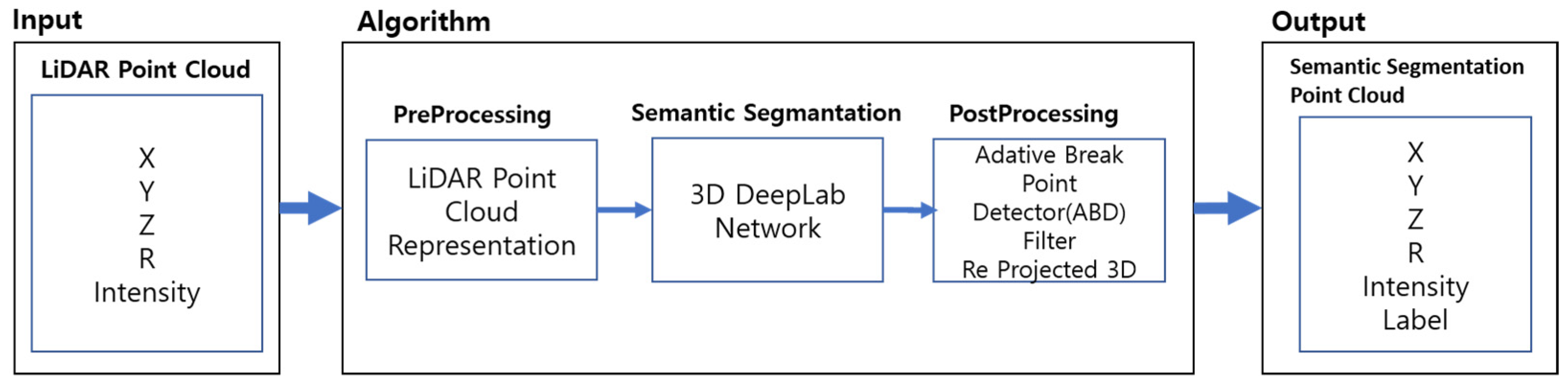
3. Method

The purpose of this study was to conduct a semantic segmentation of LiDAR data that can be used in perception systems of autonomous vehicles. The method for projecting LiDAR data into a 2D image coordinate system, and the configuration and characteristics of a DNN for a semantic segmentation of the projected image, are described in this section. Postprocessing using ABD was used to limit the misclassification during the process of recovering from the inferred image using LiDAR data. After projecting from (A) the input to the 2D image coordinate system, the semantic segmented LiDAR data were output by passing through (B) the proposed DNN and (C) the ABD filter, as shown in Figure 1.

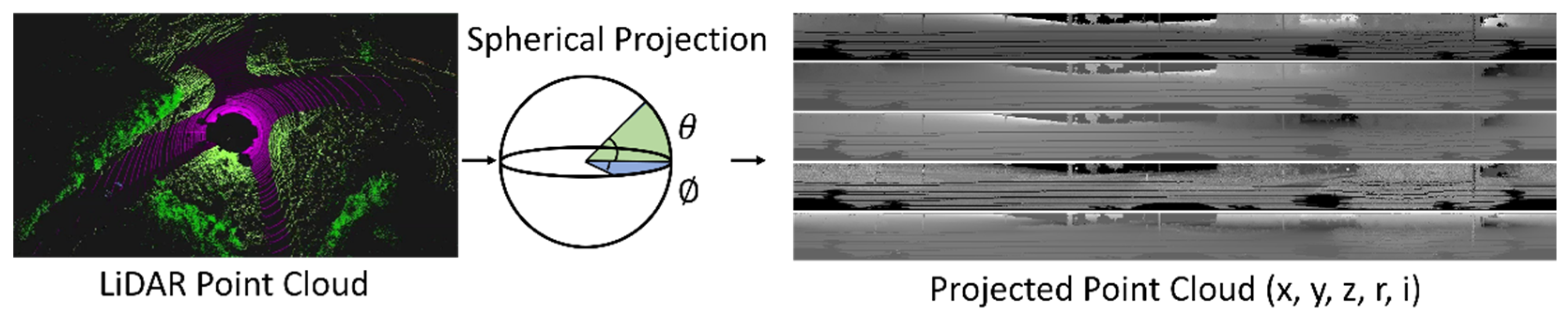
3.1. LiDAR Point Cloud Representation

The method for projecting 3D LiDAR data $\left(\mathrm{x},\mathrm{y},\mathrm{z},\mathrm{i}\right)$ onto the image coordinate system $\left(\mathrm{u},\mathrm{v}\right)$ for a 2D convolution application is described in this section. The LiDAR coordinate system can be projected onto the image coordinate system using a spherical coordinate system. The projection according to the sensor measurement method generates data with a large amount of noise, such as the overlapping of objects, when LiDAR data are projected onto the image coordinate system because 3D data are projected onto the 2D coordinate system. The data with the shortest path from the sensor are represented in the image to prevent noise. The $360°$ data acquired from the sensor are projected [11].

$$\left(\begin{array}{c}u\\ v\end{array}\right)=\left(\begin{array}{c}\frac{1}{2}\left[1-\arctan \left(y,x\right){\pi }^{-1}\right]W\\ \left[1-\left(\arcsin \left(z{r}^{-1}\right)+f_{up}\right)f^{-1}\right]H\end{array}\right),$$

(1)

where $\left(\mathrm{W},\mathrm{H}\right)$ denote the width and height of the image, and $\mathrm{x},\mathrm{y},\mathrm{z}$ denote LiDAR data. Here, $f=f_{up}+f_{down}$ is the field of view of the sensor, and $\mathrm{r}=\sqrt{x^2+y^2+z^2}$ [12]. The $\left[\mathrm{x},\mathrm{y},\mathrm{z},\mathrm{r},\mathrm{i}\right]$ image is generated by projecting the LiDAR data and $\mathrm{r}$ onto the converted coordinate system using Equation (1). The created image is input into the network in the form of $\left[W\times H\times 5\right]$. A spherical projection is shown in Figure 2.

3.2. Network Structure

The proposed network configuration uses DeepLabV3 as the main network, and partial convolution and semilocal convolution are the main convolution layer.

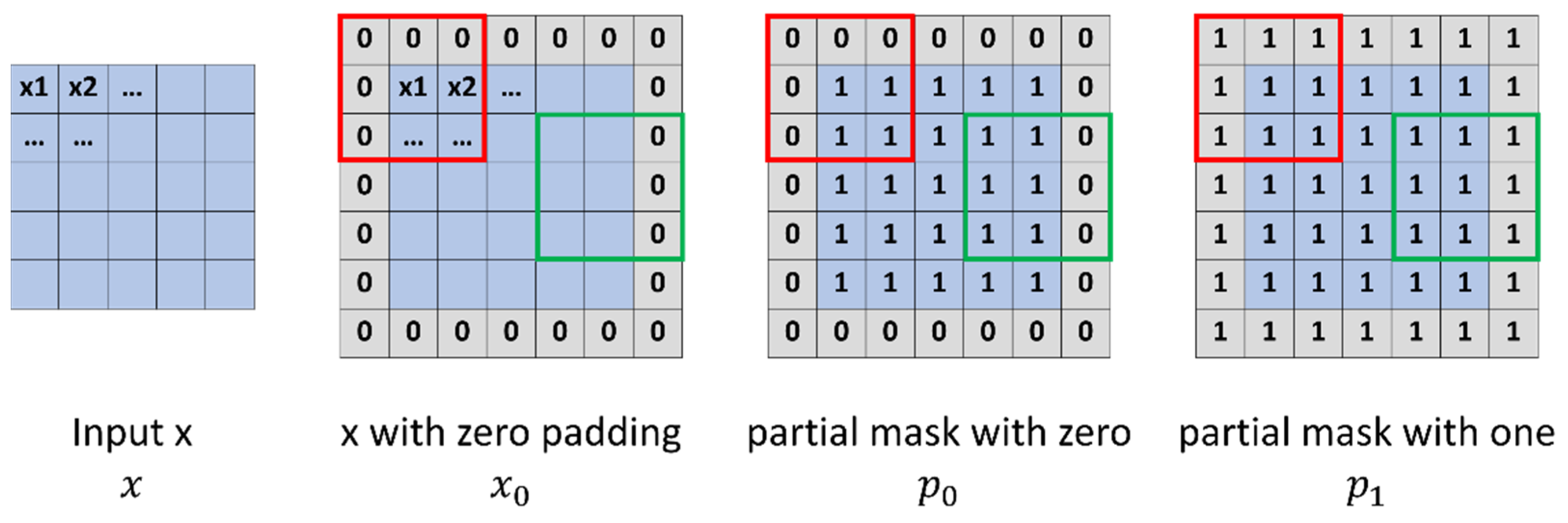
3.2.1. Partial Convolution

A partial convolution is a padding method proposed by Nvidia. The size of the input data decreases as the convolution and pooling proceed. The data may be excessively reduced, and information may be lost as the depth of the network increases. Padding is applied to extend the surroundings of the input data by filling them with a specific value to prevent data loss. Generally, zero padding is used. However, data including errors are obtained at the border of the image if it is filled with a specific value or zero. Partial convolution is a method of conditioning the output for input data by defining 0 as a hole and 1 as a non-hole by adding a binary mask. A partial convolution is helpful for data loss through the abovementioned method and has been applied to holes generated when the LiDAR data and the error at the border are projected onto a 2D coordinate system [13]. The partial convolution is shown in Figure 3.

$$\begin{gathered} \mathrm{Partial}\mathrm{conv}\left(\mathrm{x}\right)=w{x}_0*ratio \\ ratio=\frac{sum\left(p_1\right)}{sum\left(p_0\right)} \end{gathered}$$

(2)

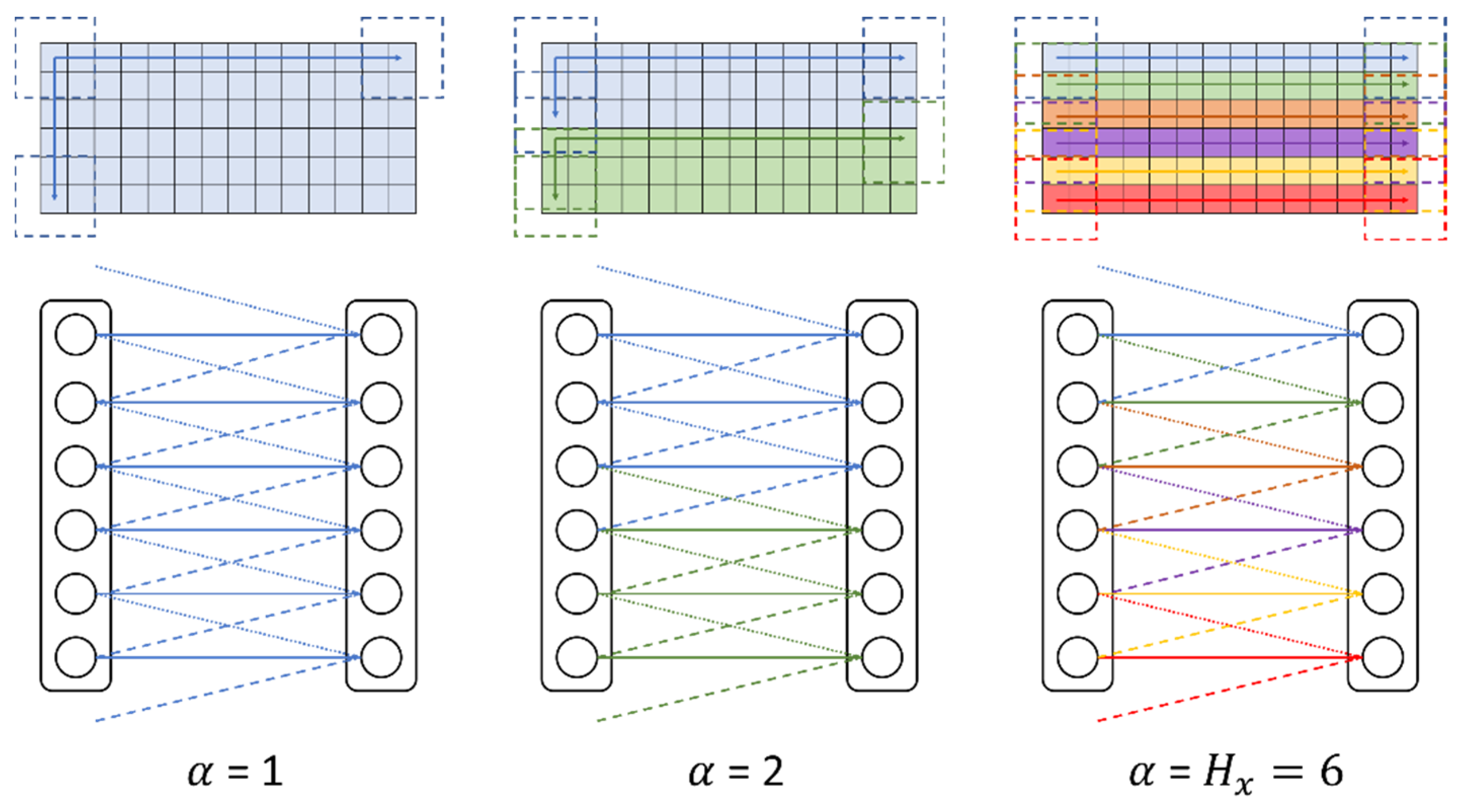
3.2.2. Semilocal Convolution

A semilocal convolution uses the fact that data in a fixed space are measured when LiDAR data are projected into a 2D coordinate system, unlike the image data of a camera. This convolution is applied by dividing the input data by $\mathsf{\alpha }$. Different kernels can be applied to the segmented convolution, and the convolution weight divided by the region is shared. Moreover, it can be learned by using the characteristics of LiDAR data because it is learned by dividing the input data by region and applying weights [14]. The semilocal convolution is shown in Figure 4.

3.2.3. Atrous Convolution

Atrous convolution creates and uses an empty space inside the kernel, unlike a conventional convolution. For segmentation, it is better for a DNN when a pixel has a wider field of view. A conventional method constructs a deeper DNN for the pixel to have a wider field of view. However, more original information is lost when the DNN is deeper. An atrous convolution expands the field of view of a pixel by creating an empty space. This is advantageous for segmentation, and a light DNN can be configured because the field of view of a pixel is expanded. Here, r represents the size of the empty space. Different ratios of r can be used to obtain multiscale features simultaneously [15]. An atrous convolution is shown in Figure 5. This convolution is used in a network, as shown in Figure 6.

3.2.4. DeepLabV3+

DeepLabV3+, used in image semantic segmentation, was applied as the backbone. DeepLabV3+ is designed for image data semantic segmentation and in encoder-decoder structures. Four methods were proposed for DeepLabV3+ from version 1 to 3+. An atrous convolution was proposed in V1, atrous spatial pyramid pooling was proposed in V2, and the ResNet structure was proposed by applying an atrous convolution in V3. The V3+ used in this study uses an atrous separable convolution [15].

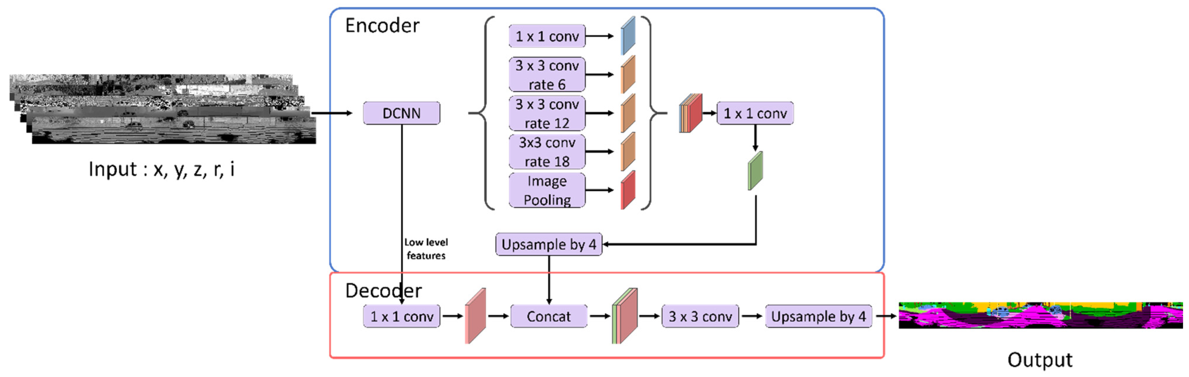
3.2.5. Network Details

Data are received in the form of $64\times 1024\times 5\left(\mathrm{H}\times \mathrm{W}\times \mathrm{C}\right)$ as input. An encoder–decoder structure is used with DeepLabV3+ as the backbone. Xception-41 is used as the backbone network, and the entry part is replaced with a partial convolution and semilocal convolution considering that the inputs are LiDAR data. Cross entropy is used as the loss function [14].

$$\mathrm{CE}\left(\widehat{y},y\right)=-{\displaystyle \sum }{\widehat{y}}_c^{i}log{y}_c^i$$

(3)

This loss function is applied most frequently. Here, ${\widehat{y}}_c^i$ denotes the ground-truth for class c at the one-hot encoded pixel position i, and $y_c^i$ denotes the predicted data of softmax. Generally, semantic segmentation is evaluated using the mean intersection over union (mIoU). The purpose is to minimize the cross entropy in the learning process to reach a high mIoU. The modified 3D model of Xception is shown in Figure 7. The network structure is shown in Figure 8.

3.3. Postprocessing

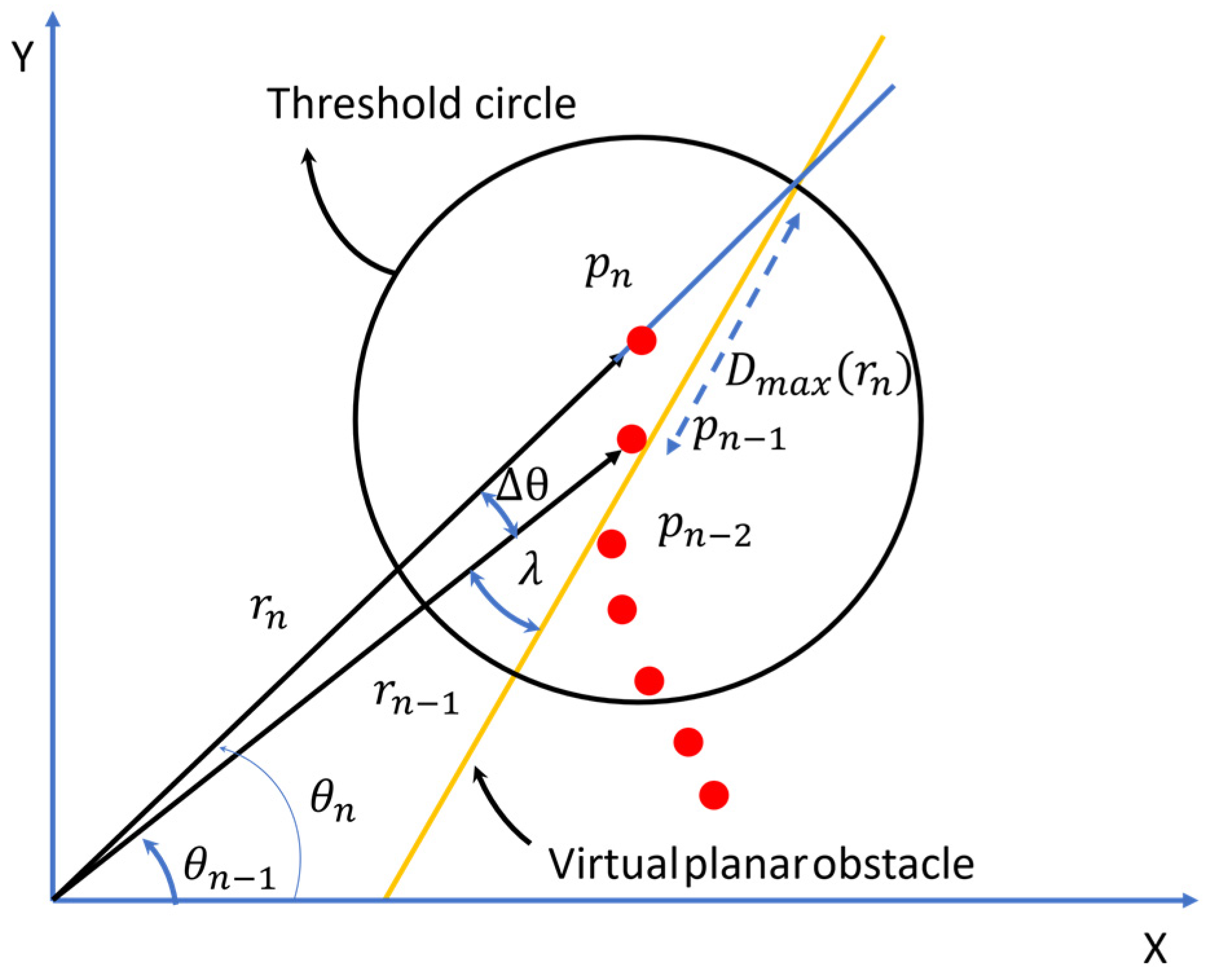
Conversion from a 3D coordinate system into a 2D coordinate system causes errors because only data with shortest path from the sensor are shown as a representative point in the 2D image coordinate system. A misclassification occurs when the data that were classified in a 2D image coordinate system are applied to 3D data. In this study, a filter using an ABD was applied to reduce the misclassification. An ABD was used for the clustering method of 2D LiDAR data.

When the distance between $||p_n-p_{n-1}||$ is greater than the threshold circle ($D_{max}$), ABD is a method that designates this as a break point [16]. If the threshold of the circle is small, the prediction will not be reached, and if it is large, an overflow will occur.

The pseudocode of the ABD, as shown in

Table 1. Adaptive break point detector.

Pseudocode: Adaptive Break Point Detector
for n = 2 to N do  $D_{max}=r_{n-1}·\frac{\sin \left(\Delta \mathsf{\Phi }\right)}{\sin \left(\lambda -\mathsf{\Delta }\mathsf{\Phi }\right)}+3{\sigma }_r$  $\mathrm{If}||p_n-p_{n-1}||>D_{max}then$   *breakpoint detected*   $fla{g}_n^b\leftarrow True$   $fla{g}_{n-1}^b\leftarrow True$  else   $fla{g}_n^b\leftarrow False$  end end

, adaptively depends on $\Delta \mathsf{\theta }$ and r, as shown in Figure 9. Here, $\Delta \mathsf{\theta }={\theta }_n-{\theta }_{n-1}$, $\mathsf{\lambda }$ denotes a user-definable constant, and ${\sigma }_r$ is the sensor noise associated with r, in which the range of influence of the circle is wider when $\mathsf{\lambda }$ is small or ${\sigma }_r$ is large. The distance r and height h of data projected on a pixel [u, v] were substituted into the filter by using the ABD as a filter in order of distance, and the classification result was applied by designating it as one object up to the break point. The parameter values were calculated empirically. In the system, $\mathsf{\lambda }$ is 10, and ${\sigma }_r$ is 2. The ABD is shown in Figure 9. The ABD postprocessing is shown in Figure 10.

4. Experiments

The network was trained and evaluated using SemanticKitti data. SemanticKitti provides LiDAR data by labeling them from Kitti data. The dataset consists of more than 43,000 scans. The data are organized in sequences within the range of 00 to 21, and 21,000 scans from 00 to 10 can be used for training because they provide the ground-truth. Sequences 11 to 21 are used as test data. The dataset provides 28 classes including moving objects, which were used in the experiment by being merged into 19 classes [10].

For the scratch training of the network, the base learning rate is 0.03, the weight decay is 0.000015, and the batch size is 38. The hardware and software configurations are presented in

Table 2. Hardware configuration.

Item	Spec
Train Desktop	Intel i9-9940X CPU 3.30 GHz Nvidia RTX-2080Ti RAM 128 GB Ubuntu 16.04
Test Desktop	Intel i7-9700E Nvidia GTX 1660Ti RAM 16 GB Ubuntu 16.04

and

Table 3. Software configuration.

Item	Spec
Language	Python 3.5
Framework	TensorFlow 1.13.2

, respectively.

An mIoU evaluation, which is mainly used in a semantic segmentation evaluation, was employed to evaluate the inference results [12]. The evaluation is shown in

Table 4. IoU [%] on test set (Sequences 11 to 21).

Approach	Pointnet++ [7]	SPGraph [17]	TrangentConv [18]	SqueezeSegV2 [2]	RangeNet53++ [12]	Proposed
						Decoder1	Decoder 2	Decoder 1
Size	50,000 pts			64 × 2048 px			64 × 1024 px
car	53.7	68.3	86.8	81.8	86.4	92.57	74.3	82.8
bicycle	1.9	0.9	1.3	18.5	24.5	42.68	15	27
motorcycle	0.2	4.5	12.7	17.9	32.7	60.33	14.4	26.8
truck	0.9	0.9	11.6	13.4	25.5	37.3	10.3	10.8
other-vehicle	0.2	0.8	10.2	14	22.6	67.31	23.4	25.8
person	0.9	1	17.1	20.1	36.2	75.78	0	3.5
bicyclist	1	6	20.2	25.1	33.6	0	25.7	0
motorcyclist	0	0	0.5	3.9	4.7	51.25	0.2	0.1
road	72	49.5	82.9	88.6	91.8	96.24	86.6	90.8
parking	18.7	1.7	15.2	45.8	64.8	70.99	56.2	66
sidewalk	41.8	24.2	61.7	67.6	74.6	91.71	67.6	73.4
other-ground	5.6	0.3	9	17.7	27.9	12.14	21.6	28.5
building	62.3	68.2	82.8	73.7	81.1	92.2	79.4	83
fence	16.9	22.5	44.2	41.1	55	75.65	42.1	53.9
vegetation	46.5	59.2	75.5	71.8	78.3	91.27	73.8	77.4
trunk	13.8	27.2	42.5	35.8	50.1	61.23	44.1	48.2
terrain	30	17	55.5	60.2	64	82.38	59.1	64.5
pole	6	18.3	30.2	20.2	38.9	56.46	23.9	32.4
traffic sign	8.9	10.5	22.2	36.3	52.2	45.8	30.5	37.3
mean IOU	20.1	20	35.9	39.7	49.9	63.33	39.4	43.8
scan/s	0.1	0.2	0.3	50	13	10	15	13

.

$$\mathrm{mIoU}=\frac{1}{C}{\displaystyle \sum }_{C=1}^C\frac{T{P}_c}{T{P}_c+F{P}_c+F{N}_c}$$

(4)

Here, $T{P}_c$,$F{P}_c$, and $F{N}_c$ are the true positive, false positive, and false negative predictions of class c, respectively, and C is the number of classes. For the evaluation network, the network was improved to apply DeepLab V3+, which is a 2D semantic segmentation network, to 3D LiDAR data as a backbone. An evaluation of the network inference results is shown in Table 4. It contains the results according to the image size and the size of the decoder stride of DeepLabV3+. The network results are shown in Figure 11.

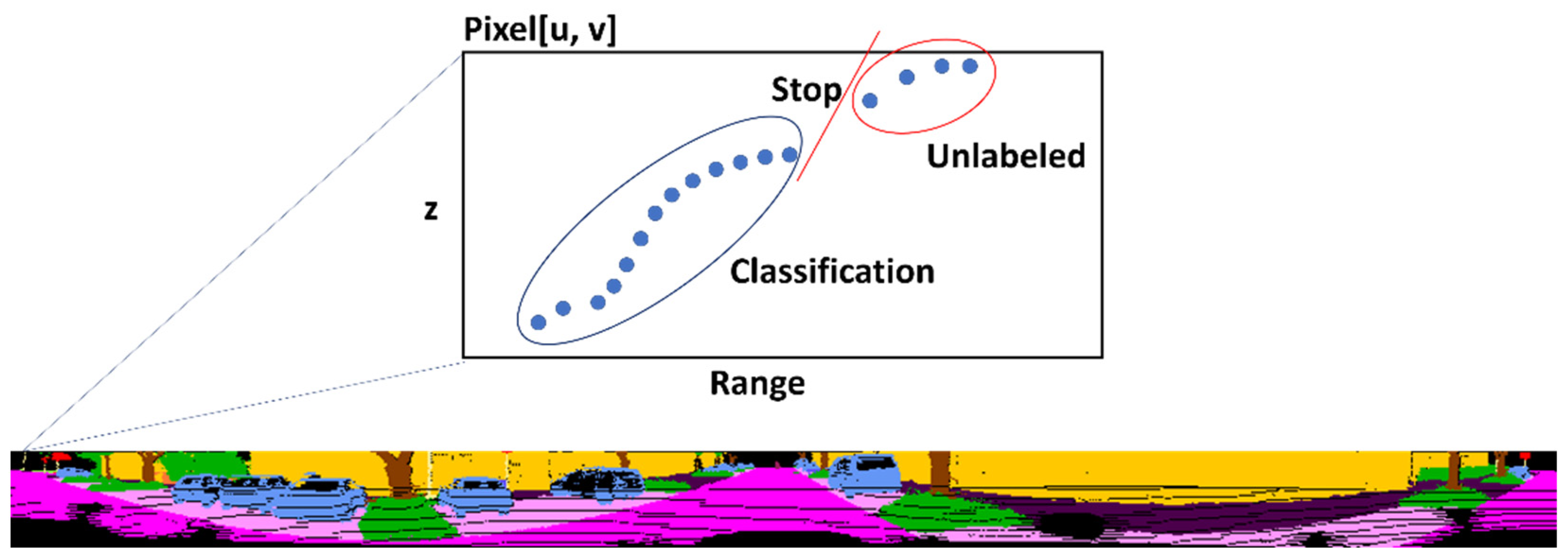
It was found that only the data projected on the 2D image were classified through the proposed filter, as shown in Figure 12. The white data are unclassified data.

5. Conclusions

A 2D network was designed for a semantic segmentation of 3D LiDAR, and a semantic segmentation algorithm using the network was proposed. The error propagation, which is a disadvantage of 2D classification, was reduced by using a postprocessed ABD filter to reduce the classification error of a 2D network. Finally, semantic segmentation was conducted for 3D LiDAR data. The practicality of this was demonstrated through its considerably faster speed than the sensor measurement speed of 10 Hz with a computing speed of 13 Hz.

A further study on the development of a network to complement classes with low classification results and for weight pruning is planned.

References

- Milioto, A.; Vizzo, I.; Behley, J.; Stachniss, C. RangeNet++: Fast and accurate LiDAR semantic segmentation. In Proceedings of the 2019 IEEE/RSJ International Conference on Intelligent Robots and Systems (IROS), Macau, China, 3–8 November 2019; pp. 4213–4220. [Google Scholar]
- Wu, B.; Wan, A.; Yue, X.; Keutzer, K. Squeezeseg: Convolutional neural nets with recurrent CRF for real-time road-object segmentation from 3D LiDAR point cloud. In Proceedings of the 2018 IEEE International Conference on Robotics and Automation (ICRA), Brisbane, Australia, 21–26 May 2018; pp. 1887–1893. [Google Scholar]
- Wu, B.; Zhou, X.; Yue, X.; Keutzer, K. Squeezesegv2: Improved model structure and unsupervised domain adaptation for road-object segmentation from a LiDAR point cloud. In Proceedings of the 2019 International Conference on Robotics and Automation (ICRA), Montreal, QC, Canada, 20–24 May 2019; pp. 4376–4382. [Google Scholar]
- Sualeh, M.; Kim, G.-W. Simultaneous localization and mapping in the epoch of semantics: A survey. Int. J. Control Autom. Syst. 2018, 17, 729–742. [Google Scholar] [CrossRef]
- Kang, D.W.; Kim, D.J.; Sun, H.D.; Kim, J.H. Object classification and optimize calibration using the network in map. J. Inst. Control Robot. Syst. 2020, 26, 443–451. [Google Scholar] [CrossRef]
- Sandler, M.; Howard, A.; Zhu, M.; Zhmoginov, A.; Chen, L. MobileNetV2: Inverted residuals and linear bottlenecks. In Proceedings of the IEEE Conference on Computer Vision and Pattern Recognition, Salt Lake City, UT, USA, 18–23 June 2018; pp. 4510–4520. [Google Scholar]
- Qi, C.R.; Su, H.; Mo, K.; Guibas, L.J. PointNet: Deep learning on point sets for 3D classification and segmentation. In Proceedings of the IEEE Conference on Computer Vision and Pattern Recognition (CVPR), Las Vegas, NV, USA, 27–30 June 2016; pp. 652–660. [Google Scholar]
- Qi, C.R.; Yi, K.; Su, H.; Guibas, L.J. PointNet++: Deep hierarchical feature learning on point sets in a metric space. In Proceedings of the Advances in Neural Information Processing Systems (NIPS), Long Beach, CA, USA, 4–9 December 2017; pp. 5105–5114. [Google Scholar]
- Zhou, Y.; Tuzel, O. Voxelnet: End-to-end learning for point cloud based 3D object detection. In Proceedings of the IEEE Conference on Computer Vision and Pattern Recognition, Salt Lake City, UT, USA, 18–23 June 2018; pp. 4490–4499. [Google Scholar]
- Neuhold, G.; Ollmann, T.; Bulo, S.R.; Kontschieder, P. The Mapillary vistas dataset for semantic understanding of street scenes. In Proceedings of the IEEE Intl. Conference on Computer Vision (ICCV), Venice, Italy, 22–29 October 2017; pp. 4990–4999. [Google Scholar]
- Behley, J.; Garbade, M.; Milioto, A.; Quenzel, J.; Behnke, S.; Stachniss, C.; Gall, J. SemanticKITTI: A dataset for semantic scene understanding of LiDAR sequences. In Proceedings of the IEEE/CVF International Conference on Computer Vision (ICCV), Seoul, South Korea, 27 October–3 November 2019; pp. 9297–9307. [Google Scholar]
- Park, S.Y.; Choi, S.I.; Moon, J.; Kim, J.; Park, Y.W. Localization of an unmanned ground vehicle based on hybrid 3D registration of 360degree range data and DSM. Int. J. Control Autom. Syst. 2011, 9, 875–887. [Google Scholar] [CrossRef]
- Liu, G.; Shih, K.J.; Wang, T.C.; Reda, F.A.; Sapra, K.; Yu, Z.; Catanzaro, B. Partial convolution based padding. arXiv 2018, arXiv:1811.11718. [Google Scholar]
- Triess, L.T.; Peter, D.; Rist, C.B.; Zöllner, J.M. Scan-based semantic segmentation of LiDAR point clouds: An experimental study. In Proceedings of the 2020 IEEE Intelligent Vehicles Symposium (IV), Las Vegas, NV, USA, 19 October–13 November 2020; pp. 1116–1121. [Google Scholar]
- Chen, L.C.; Zhu, Y.; Papndreou, G.; Schroff, F.; Adam, H. Encoder-decoder with atrous separable convolution for semantic image segmentation. In Proceedings of the European Conference on Computer Vision (ECCV), Munich, Germany, 8–14 September 2018; pp. 801–818. [Google Scholar]
- Kang, D.W.; Yang, J.H.; Kim, J.H. Extended Kalman filter based localization to autonomous vehicles using a 2D laser sensor. In Proceedings of the Korean Society of Automotive Engineers, Jeju, Korea, 18–20 May 2017; pp. 493–497. [Google Scholar]
- Landrieu, L.; Simonovsky, M. Large-scale point cloud semantic segmentation with superpoint graphs. In Proceedings of the IEEE Conference on Computer Vision and Pattern Recognition (CVPR), Salt Lake City, UT, USA, 18–23 June 2018; pp. 4558–4567. [Google Scholar]
- Tatarchenko, M.; Park, J.; Koltun, V.; Zhou, Q.-Y. Tangent convolutions for dense prediction in 3D. In Proceedings of the IEEE Conference on Computer Vision and Pattern Recognition (CVPR), Salt Lake City, UT, USA, 18–23 June 2018; pp. 3887–3896. [Google Scholar]