
Diagnosis of Alzheimer’s Disease Based on the Modified Tresnet

Abstract
:
1. Introduction
2. Related Work
3. Materials and Methodology
3.1. Data Acquisition
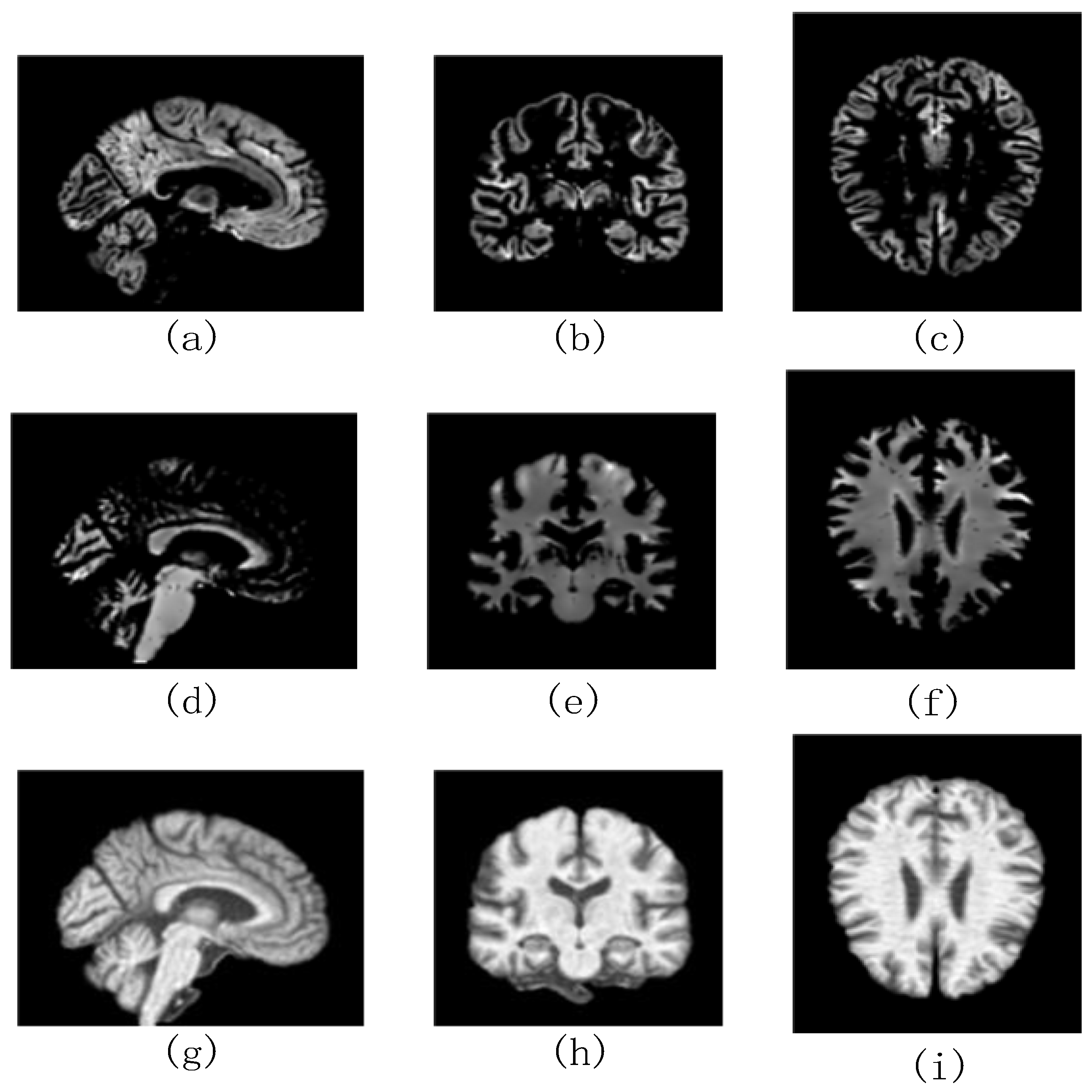
3.2. Data Preprocessing
3.2.1. MRI Data Processing Flow
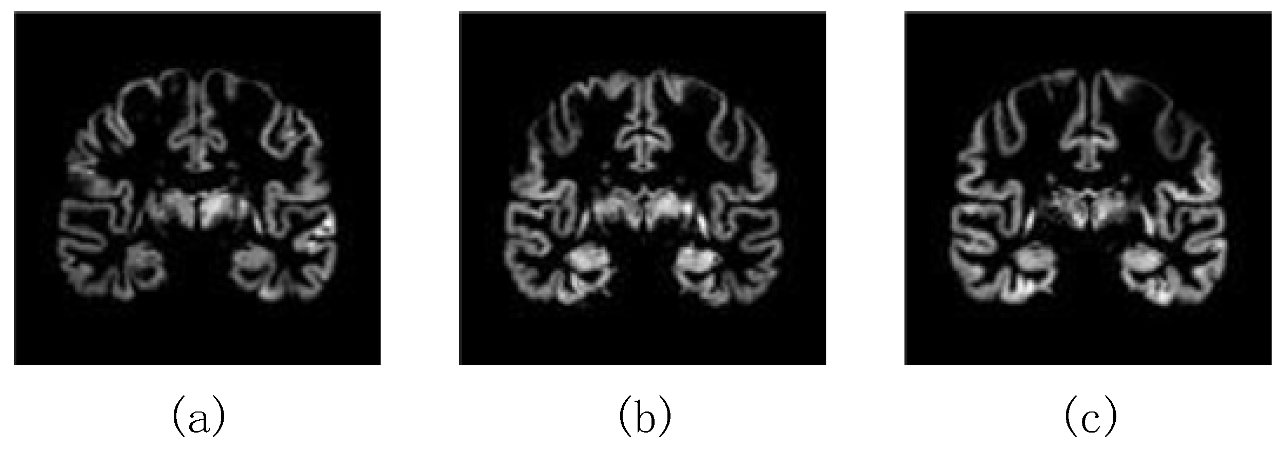
3.2.2. The Choice of the Most Informative Slices
3.3. Methodology
3.3.1. Tresnet
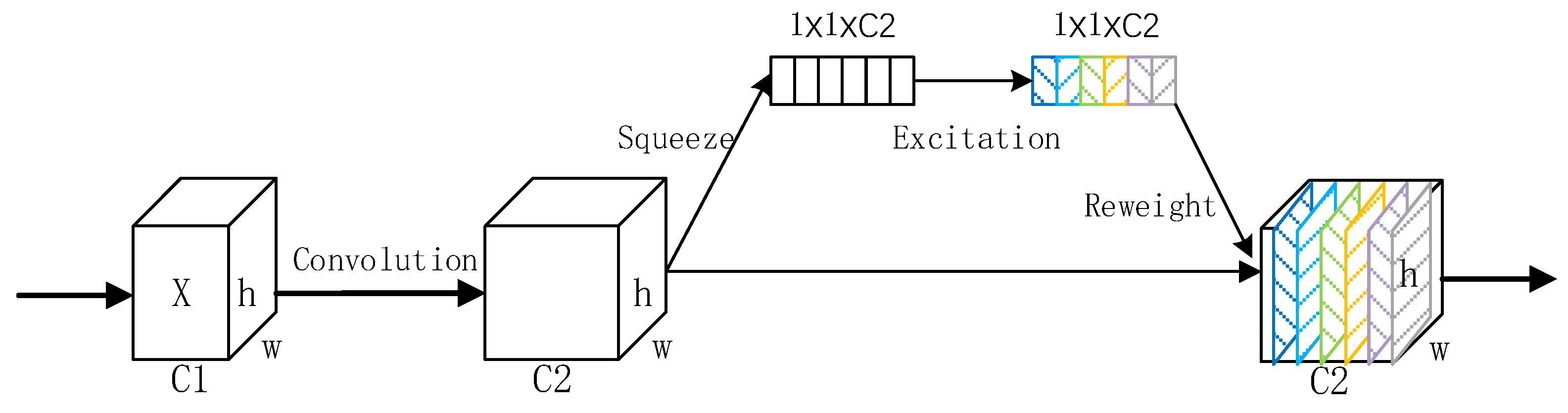
3.3.2. SK Module
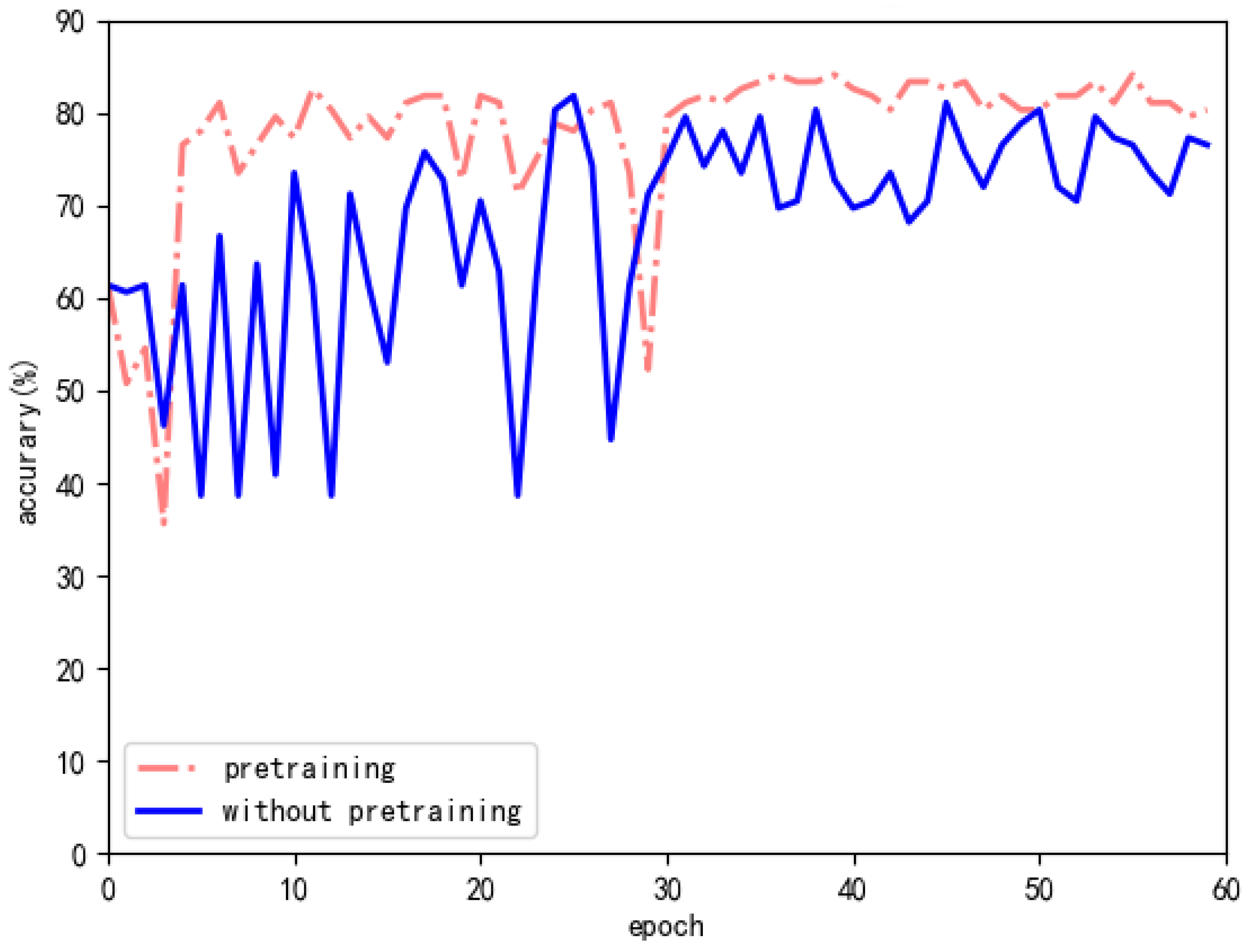
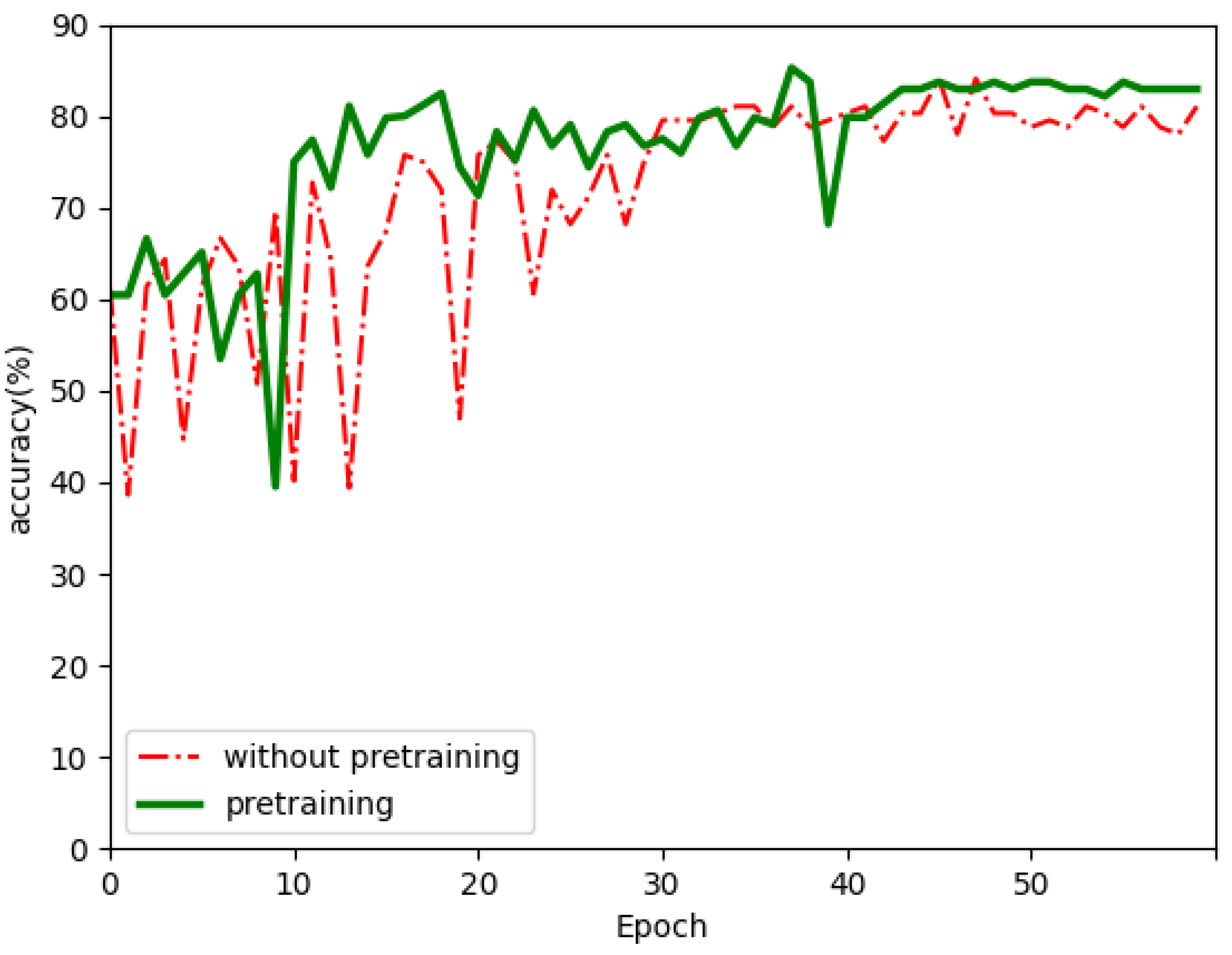
3.3.3. Transfer Learning
4. Evaluation Metrics and Experimental Results
5. Discussion
6. Conclusions
Author Contributions
Funding
Conflicts of Interest
References
- Vatanabe, I.P.; Manzine, P.R.; Cominetti, M.R. Historic concepts of dementia and Alzheimer’s disease: From ancient times to the present. Rev. Neurol. 2020, 173, 140–147. [Google Scholar] [CrossRef] [PubMed]
- Sundberg, R.J.; Adlard, E.R. The chemical century: Molecular manipulation and its impact on the 20th century. Chromatographia 2017, 80, 1599. [Google Scholar]
- Fan, Z.; Xu, F.Y.; Qi, X.D.; Li, C.; Yao, L. Classification of Alzheimer’s disease based on brain MRI and machine learning. Neural Comput. Appl. 2020, 32, 1927–1936. [Google Scholar] [CrossRef]
- Yildirim, M.; Cinar, A. Classification of Alzheimer’s disease MRI Images with CNN based hybrid method. Ing. Syst. D Inf. 2020, 25, 413–418. [Google Scholar]
- Carrillo, M.C.; Bain, L.J.; Frisoni, G.B.; Weiner, M.W. Worldwide Alzheimer’s disease neuroimaging initiative. Alzheimers Dement. 2012, 8, 337–342. [Google Scholar] [CrossRef] [PubMed]
- Kadmiri, N.E.; Said, N.; Slassi, I.; El Moutawakil, B.; Nadifi, S. Biomarkers for Alzheimer disease: Classical and novel candidates review. Neuroscience 2018, 370, 181–190. [Google Scholar] [CrossRef]
- Liu, J.; Pan, Y.; Wu, F.X.; Wang, J. Enhancing the feature representation of multi-modal MRI data by combining multi-view information for MCI classification. Neurocomputing 2020, 400, 322–332. [Google Scholar] [CrossRef]
- Suk, H.I.; Lee, S.W.; Shen, D. Hierarchical feature representation and multimodal fusion with deep learning for AD/MCI diagnosis. Neurocomputing 2014, 101, 569–582. [Google Scholar] [CrossRef] [Green Version]
- Tzimourta, K.D.; Christou, V.; Tzallas, A.T.; Giannakeas, N.; Astrakas, L.G.; Angelidis, P.; Tsalikakis, D.; Tsipouras, M.G. Machine Learning Algorithms and Statistical Approaches for Alzheimer’s Disease Analysis Based on Resting-State EEG Recordings: A Systematic Review. Int. J. Neural Syst. 2020, 31, 2130002. [Google Scholar] [CrossRef]
- Yang, S.; Bornot, J.M.S.; Wong-Lin, K.; Prasad, G. M/EEG-based bio-markers to predict the MCI and Alzheimer’s disease: A review from the ML perspective. IEEE Trans. Biomed. Eng. 2019, 66, 2924–2935. [Google Scholar] [CrossRef] [PubMed]
- Khan, M.A.; Kim, Y. Cardiac arrhythmia disease classification using LSTM deep learning approach. Comput. Mater. Contin. 2021, 67, 427–446. [Google Scholar] [CrossRef]
- Al-Shoukry, S.; Rassem, T.H.; Makbol, N.M. Alzheimer’s diseases detection by using deep learning algorithms: A Mini-Review. IEEE Access 2020, 8, 77131–77141. [Google Scholar] [CrossRef]
- Liu, S.Q.; Liu, S.D.; Cai, W.D. Multimodal neuroimaging feature learning for multiclass diagnosis of Alzheimer’s disease. IEEE Trans. Biomed. Eng. 2015, 62, 1132–1140. [Google Scholar] [CrossRef] [Green Version]
- Shen, K.K.; Fripp, J.; Mériaudeauet, J. Detecting global and local hippocampal shape changes in Alzheimer’s disease using statistical shape models. Neuroimage 2012, 58, 2155–2166. [Google Scholar] [CrossRef] [PubMed]
- Moradi, E.; Pepe, A.; Gaser, C.; Huttunen, H.; Tohka, J. Alzheimer’s Disease Neuroimaging Initiative. Machine learning framework for early MRI-based Alzheimer’s conversion prediction in MCI subjects. Neuroimage 2015, 104, 398–412. [Google Scholar] [CrossRef] [PubMed] [Green Version]
- Zhang, Y.P.; Wang, S.H.; Xia, K.J.; Jiang, Y.; Qian, P. Alzheimer’s disease multiclass diagnosis via multimodal neuroimaging embedding feature selection and fusion. Inf. Fusion 2021, 66, 170–183. [Google Scholar] [CrossRef]
- Li, S.; Shi, F.; Pu, F.; Li, X.; Jiang, T.; Xie, S.; Wang, Y. Hippocampal shape analysis of Alzheimer disease based on machine learning methods. Am. J. Neuroradiol. 2007, 28, 1339–1345. [Google Scholar] [CrossRef] [Green Version]
- Gunawardena, K.; Rajapakse, R.N.; Kodikara, N.D. Applying convolutional neural networks for pre-detection of Alzheimer’s disease from structural MRI data. In Proceedings of the 2017 24th International Conference on Mechatronics and Machine Vision in Practice(M2VIP), Auckland, New Zealand, 21–23 November 2017. [Google Scholar]
- Aderghal, K.; Benois-Pineau, J.; Karim, A. FuseMe: Classification of sMRI images by fusion of deep CNNs in 2D+ projections. In Proceedings of the International Workshop on Content-Based Multimedia Indexing, Firenze, Italy, 19–21 June 2017. [Google Scholar]
- Korolev, S.; Safiullin, A.; Belyaev, M. Residual and plain convolutional neural networks for 3D brain MRI classification. In Proceedings of the IEEE International Symposium on Biomedical Imaging 2017, Melbourne, Australia, 26 September 2017; pp. 835–838. [Google Scholar]
- Valliani, A.; Soni, A. Deep Residual Nets for Improved Alzheimer’s Diagnosis; ACM: Hannover, Germany, 2017; p. 615. [Google Scholar]
- Cheng, D.; Liu, M. CNNs based multi-modality classification for AD diagnosis. In Proceedings of the 2017 10th International Congress on Image and Signal Processing, BioMedical Engineering and Informatics(CISP-BMEI), Shanghai, China, 14–16 October 2017. [Google Scholar]
- Lin, W.L.; Tong, T.; Gao, Q.Q. Convolutional neural networks-based MRI image analysis for the Alzheimer’s disease prediction from mild cognitive impairment. Front. Neurosci. 2018, 12, 777. [Google Scholar] [CrossRef]
- Kanghan, O.; Chung, Y.C.; Kim, K.W. Classification and visualization of Alzheimer’s disease using volumetric convolutional neural network and transfer learning. Nature 2019, 9, 5663–5679. [Google Scholar]
- Wen, J.H.; Thibeau-Sutre, E.; Diaz-Melo, M. Convolutional neural networks for classification of Alzheimer’s disease: Overview and reproducible evaluation. Med. Image Anal. 2020, 63, 101694–101713. [Google Scholar] [CrossRef]
- Lin, L.; Zhang, B.W.; Wu, S.C. Hybrid CNN-SVM for alzheimer’s disease classification from structural MRI and the alzheimer’s disease neuroimaging initiative(ADNI). In Proceedings of the 2018 International Conference on Biomedical Engineering, Machinery and Earth Science (BEMES 2018), Guangzhou, China, 1 September 2018. [Google Scholar]
- Liu, M.; Zhang, D.; Shen, D. Ensemble sparse classification of Alzheimer’s disease. Neuroimagel 2012, 60, 1106–1116. [Google Scholar] [CrossRef] [PubMed] [Green Version]
- Ridnik, T.; Lawen, H.; Noy, A.; Friedman, I.; Baruch, E.B.; Sharir, G. TResNet: High performance GPU-dedicated architecture. In Proceedings of the IEEE/CVF Winter Conference on Applications of Computer Vision (WACV), Aspen, CO, USA, 1–5 March 2020; pp. 1400–1409. [Google Scholar]
- Li, X.; Wang, W.; Hu, X.X.; Yang, J. Selective kernel networks. In Proceedings of the IEEE/CVF Conference on Computer Vision and Pattern Recognition (CVPR) IEEE, Los Angeles, CA, USA, 1 March 2019; pp. 510–519. [Google Scholar]
- Litjens, G.; Kooi, T.; Bejnordi, B.E.; Setio, A.A.A.; Sánchez, C.I. A survey on deep learning in medical image analysis. Med. Image Anal. 2017, 42, 60–88. [Google Scholar] [CrossRef] [PubMed] [Green Version]
- Yosinski, J.; Clune, J.; Bengio, Y.; Lipson, H. How transferable are features in deep neural networks? In Proceedings of the Neural Information Processing Systems (NIPS), Montreal, QC, Canada, 6 November 2014. [Google Scholar]


| Daignosis | Age | Sex (Male (M)/Female (F)) |
|---|---|---|
| AD | 73.63 ± 7.68 | 43 M/42 F |
| MCI | 73.82 ± 7.47 | 156 M/88 F |
| NC | 75.29 ± 4.85 | 75 M/58 F |
| Layer | Block | Output | Stride | Tresenet+SK | |
|---|---|---|---|---|---|
| Repeats | Channnels | ||||
| Stem | SpaceToDepth | 56 × 56 | - | 1 | 48 |
| Conv 1 × 1 | 1 | 1 | 76 | ||
| Stage 1 | BasicBlock+SK | 56 × 56 | 1 | 4 | 76 |
| Stage 2 | BasicBlock+SK | 28 × 28 | 2 | 5 | 152 |
| Stage 3 | Bottleneck+SK | 14 × 14 | 2 | 18 | 1216 |
| Stage 4 | Bottleneck | 7 × 7 | 2 | 3 | 2432 |
| Pooling | GlobalAvgPool | 1 × 1 | 1 | 1 | 2432 |
| Params | 52.0 M | ||||
| Network Model | AD vs. NC | AD vs. MCI vs. NC |
|---|---|---|
| LeNet | 79.5% | 55.6% |
| Resnet | 82.1% | 58.6% |
| Mobilenetv2 | 82.6% | 59.1% |
| Densenet | 83.9% | 58.8% |
| Tresnet | 84.8% | 58.2% |
| Tresnet+SK | 85.9% | 61.8% |
| Network Model | SEN | SPE | F1 |
|---|---|---|---|
| LeNet | 76.5% | 82.6% | 78% |
| Resnet | 79.2% | 85.9% | 80.6% |
| Mobilenetv2 | 77.2% | 89.1% | 80% |
| Densenet | 81% | 88.6% | 82.4% |
| Tresnet | 81.9% | 88% | 83.3% |
| Tresnet+SK | 82.1% | 88.3% | 83.9% |
| Model | AD vs. NC | AD vs. MCI vs. NC |
|---|---|---|
| Tresnet_M | 84.4% | 58.2% |
| Tresnet_M+SK | 84.8% | 59.7% |
| Tresnet_L | 84.9% | 58.9% |
| Tresnet_L+SK | 85.9% | 61.8% |
| Tresnet_XL | 84.1% | 57.6% |
| Tresnet_XL+SK | 84.8% | 58.3% |
| Model | SEN | SPE | F1 |
|---|---|---|---|
| Tresnet_M | 80.4% | 87.5% | 82.4% |
| Tresnet_M+SK | 81.5% | 87.5% | 83.1% |
| Tresnet_L | 80.9% | 87.3% | 82.9% |
| Tresnet_L+SK | 82.1% | 88.3% | 83.9% |
| Tresnet_XL | 80.4% | 87.1% | 82.2% |
| Tresnet_XL+SK | 80.6% | 87.7% | 82.7% |
| Method | Dataset | AD vs. NC | 3-Ways |
|---|---|---|---|
| Korolev et al. [20] 3D CNN | 50 AD + 120 MCI + 61 NC | 80.0% | - |
| Valliani et al. [21] 2D CNN | 188 AD + 243 MCI + 229 NC | 81.3% | 56.8% |
| Cheng et al. (MRI) [22] 3D CNN | 193 AD + MCI + NC | 85.5% | - |
| Zhang et al. [16] SVM | 38 AD + 42 MCI + 40 NC | 87.7% | 84% |
| Wen et al. [25] 2D CNN 3D subject-level CNN 3D path-level CNN SVM | 336 AD + 787 MCI + 330 NC | 82% 83.5% 78% 88% | - |
| Lin et al. [23] 3D multi-model | 193 AD + 151 NC | 77% | - |
| Kanghan et al. [24] 3D CNN | 198 AD + 230 NC | 86.6% | - |
| Proposed | 85 AD + 244 MCI + 133 NC | 86.9% | 63.2% |
| Method | Dataset | SEN | SPE | F1 |
|---|---|---|---|---|
| Korolev et al. [20] | 50 AD + 120 MCI + 61 NC | 79.3% | 73.9% | 79.6% |
| Cheng et al. (MRI) [21] | 193 AD + MCI + NC | 83.8% | 90% | 84.6% |
| Kanghan et al. [24] | 198 AD + 230 NC | 88.5% | 84.5% | 92.8% |
| Proposed | 85 AD + 244 MCI + 133 NC | 84% | 88.7% | 85.4% |
| Model | Tresnet+SK | |
|---|---|---|
| AD vs. NC | AD vs. MCI vs. NC | |
| GM+WM | 82.9% | 56.2% |
| WM | 82.1% | 56.9% |
| GM | 85.9% | 61.8% |
| Model | Tresnet+SK | ||
|---|---|---|---|
| SEN | SPE | F1 | |
| GM+WM | 78.9% | 82.1% | 80.9% |
| WM | 78.3% | 83.1% | 80.2% |
| GM | 82.1% | 88.3% | 84.4% |
| Model | AD vs. NC | AD vs. MCI vs. NC |
|---|---|---|
| without pretraining | ACC: 85.9% SEN: 82.1% SPE: 88.3% F1: 83.9% | ACC: 61.8% |
| pretraining | ACC: 86.9% SEN: 84% SPE: 88.7% F1: 85.4% | ACC: 63.2% |
Publisher’s Note: MDPI stays neutral with regard to jurisdictional claims in published maps and institutional affiliations. |
© 2021 by the authors. Licensee MDPI, Basel, Switzerland. This article is an open access article distributed under the terms and conditions of the Creative Commons Attribution (CC BY) license (https://creativecommons.org/licenses/by/4.0/).
Share and Cite
Xu, Z.; Deng, H.; Liu, J.; Yang, Y. Diagnosis of Alzheimer’s Disease Based on the Modified Tresnet. Electronics 2021, 10, 1908. https://doi.org/10.3390/electronics10161908
Xu Z, Deng H, Liu J, Yang Y. Diagnosis of Alzheimer’s Disease Based on the Modified Tresnet. Electronics. 2021; 10(16):1908. https://doi.org/10.3390/electronics10161908
Chicago/Turabian StyleXu, Zelin, Hongmin Deng, Jin Liu, and Yang Yang. 2021. "Diagnosis of Alzheimer’s Disease Based on the Modified Tresnet" Electronics 10, no. 16: 1908. https://doi.org/10.3390/electronics10161908
APA StyleXu, Z., Deng, H., Liu, J., & Yang, Y. (2021). Diagnosis of Alzheimer’s Disease Based on the Modified Tresnet. Electronics, 10(16), 1908. https://doi.org/10.3390/electronics10161908