
A Novel Metaheuristic Moss-Rose-Inspired Algorithm with Engineering Applications


Abstract
:1. Introduction
2. Moss Rose Optimization Algorithm
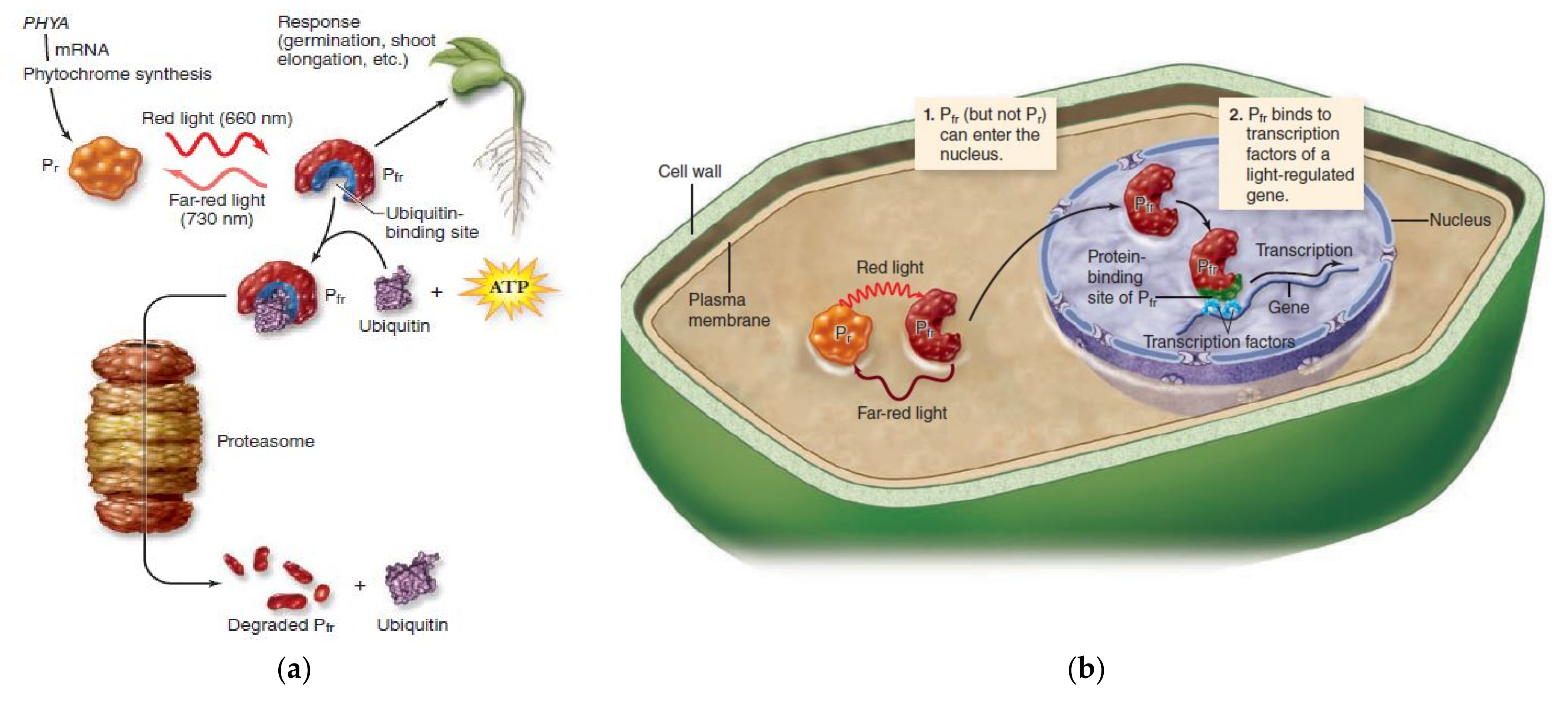
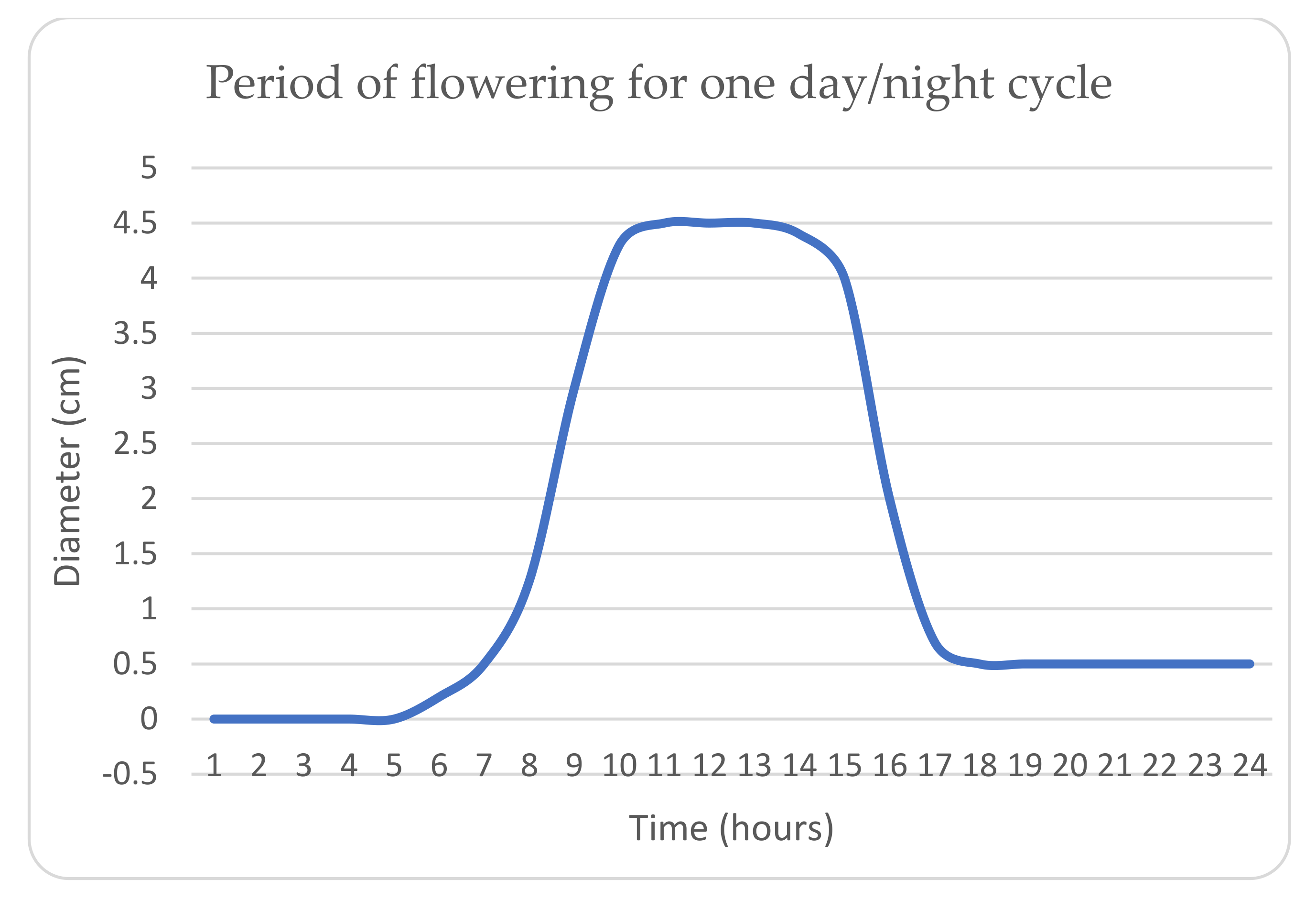
2.1. Inspiration
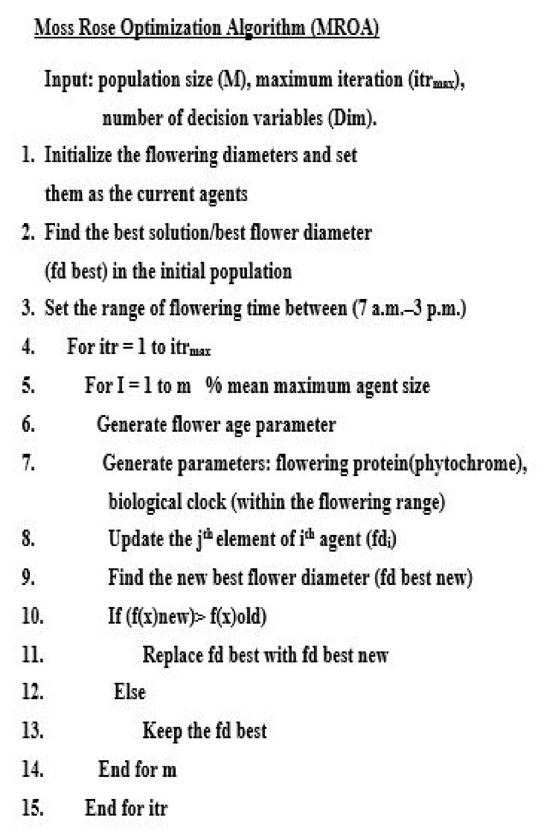
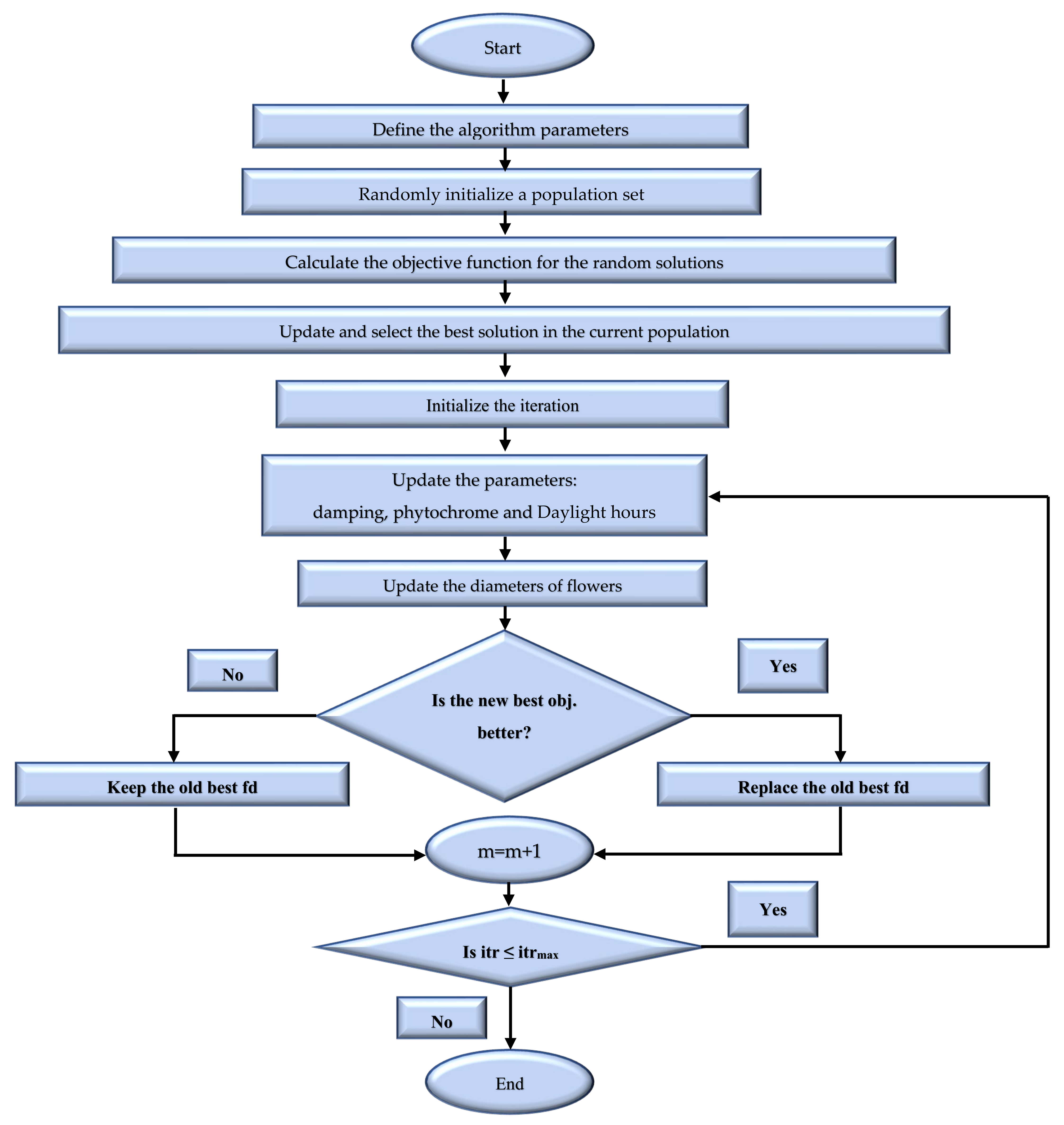
2.2. Mathematical Model
- Create random variables that represent the flowering diameters:where —the diameters of roses between max and min values.
- Generate the flowering age parameter, which depends on the current diameter and the maximum diameter that the flower will reach. The equation for the iswhere —maximum flower diameter and —total hours in a day.
- Generate the phytochrome parameter, which depends on the max flowering diameter, the number of hours the flowers are open, a random time in the morning and the minimum flowering diameter:where BF—biological opening factor (controls the clock time of flowering; the value is 3), SF—scaling factor (to ensure the maximum reaction of the rose to light effect; the value is 2.7), —maximum number of hours the flowers are open and —minimum flower diameter.
- Calculate the new fd according to the following equation:where Pr—red photon wavelength (nm) and —best flowering diameter, which is calculated based on the fitness function.
3. Computational Results of Benchmark Functions
- (a)
- Unimodal functions for benchmarking;
- (b)
- Functions for multimodal benchmarks.
4. Engineering Optimization Applications
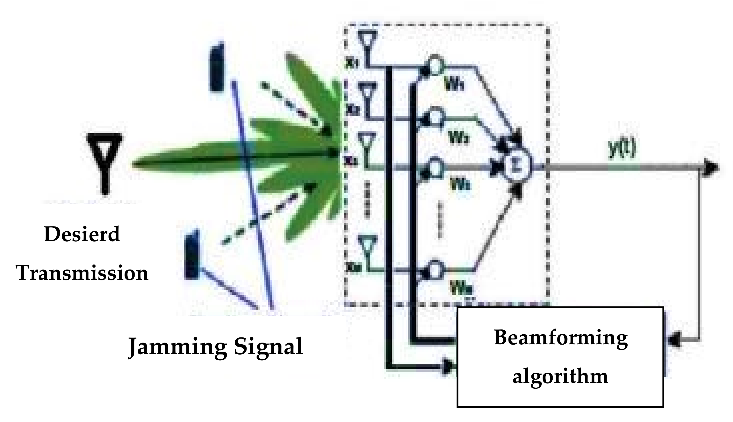
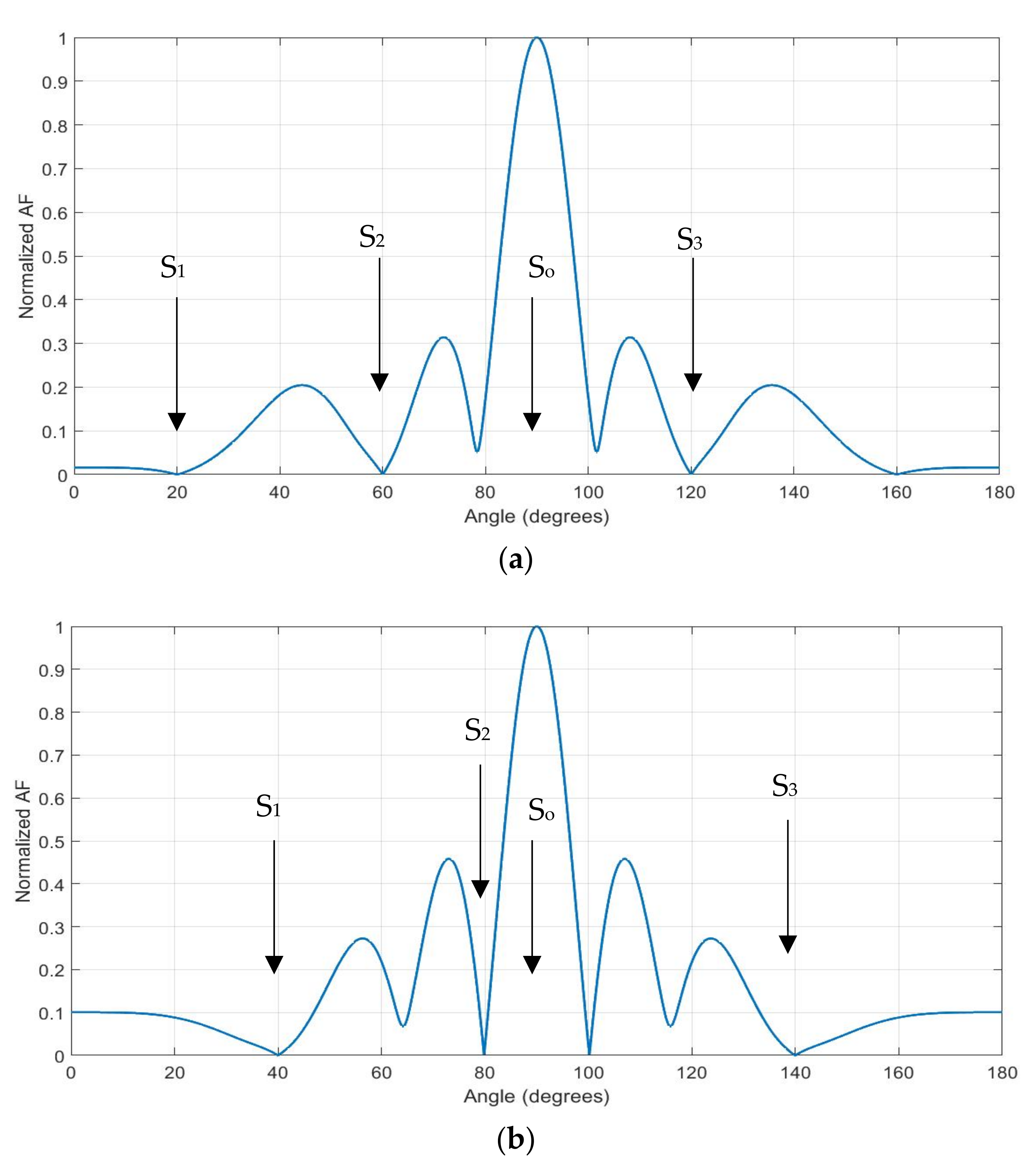
4.1. Smart Antennas with Anti-Jamming
- Case 1:
- Case 2:
- Case 3:
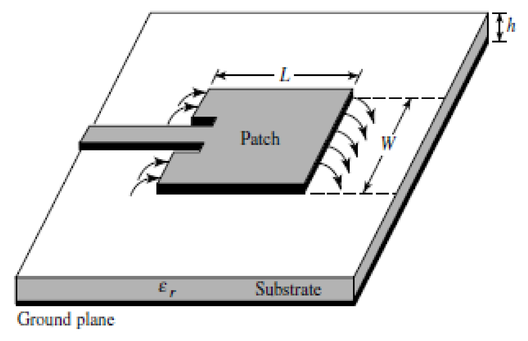
4.2. Narrowband Microstrip Patch Antenna Design
- Specify the center frequency and choose a permittivity () and the thickness of the substrate (h):
- Find the patch width (Wp) usingwhere is the light velocity, and is the resonant frequency.
- Calculate the effective dielectric constant using the following equation:
- Calculate the extended length ():
- Calculate the patch length (Lp) using the following equation:
- Find the notch width using the following equation:
- Calculate the matching impedance Zo as follows:where the input impedance (Rin) is obtained using
5. Conclusions
- Generate random variables.
- Identify the values of the variables that produced the best solution to the calculated fitness function.
- Generate a new variable representing the lifetime of the variable.
- Generating a second variable that represents the extent of the influence of natural factors upon updating the variable data.
- Update the variables and compare the results with the previous results to obtain convergence toward a better outcome.
Author Contributions
Funding
Acknowledgments
Conflicts of Interest
References
- Yang, X.-S. Nature-Inspired Optimization Algorithms, 1st ed.; Elsevier Inc.: Amsterdam, The Netherlands, 2014. [Google Scholar]
- Dorigo, M. Optimization, Learning and Natural Algorithms. Ph.D. Thesis, Politecnico di Milano, Milan, Italy, 1992. [Google Scholar]
- Kennedy, J.; Eberhart, R. Particle swarm optimization. In Proceedings of the IEEE CNN’95 International Conference on Neural Networks, Perth, WA, Australia, 27 November–1 December 1995; Volume 4, pp. 1942–1948. [Google Scholar]
- Mehrabian, A.; Lucas, C. A novel numerical optimization algorithm inspired from weed colonization. In Ecological Informatics; Elsevier: Amsterdam, The Netherlands, 2006; pp. 355–366. [Google Scholar]
- Yang, X.-S. Firefly Algorithms for Multimodal Optimization; Springer: Berlin/Heidelberg, Germany, 2009; pp. 169–178. [Google Scholar]
- Yang, X.-S. Engineering optimization by cuckoo search. Int. J. Math. Model. Numer. Optim. 2010, 1, 330–343. [Google Scholar]
- Yang, X.-S. A New Metaheuristic Bat-Inspired Algorithm, Nature-Inspired Cooperative Strategies for Optimization (NICSO); Springer: Cham, Switzerland, 2010; Volume 284, pp. 65–74. [Google Scholar]
- Yang, X.-S. Flower Pollination Algorithm for Global Optimization Lecture Notes in Computer Science; Springer: Cham, Switzerland, 2012; pp. 240–249. [Google Scholar]
- Hao, Z.; Yunlong, Z.; Hanning, C. Root Growth Model: A Novel Approach to Numerical Function Optimization and Simulation of Plant Root System; Springer: Cham, Switzerland, 2013. [Google Scholar]
- Seyedali, M.; Andrew, L. The Whale Optimization Algorithm Advances in Engineering Software; Elsevier Ltd.: Amsterdam, The Netherlands, 2016. [Google Scholar]
- Nancy, G.; Jyoti, S.; Kamaljit, S. Bhatia, Design Optimization of CPW-Fed Microstrip Patch Antenna Using Constrained ABFO Algorithm; Springer: Cham, Switzerland, 2017. [Google Scholar]
- Mohit, J.; Vijander, S.; Asha, R. A novel nature-inspired algorithm for optimization: Squirrel search algorithm. In ScienceDirect. Swarm and Evolutionary Computation; Elsevier Ltd.: Amsterdam, The Netherlands, 2018. [Google Scholar]
- Ali, R.S.; Alnahwi, F.M.; Abdulkareem, S.A. A modified camel travelling behaviour algorithm for engineering applications. Aust. J. Electr. Electron. Eng. 2019, 16, 176–186. [Google Scholar] [CrossRef]
- Sattar, D.; Salim, R. A smart metaheuristic algorithm for solving engineering problems. Eng. Comput. 2020, 1–29. [Google Scholar] [CrossRef]
- Kirkpatrick, S.; Gelatt, C.D.; Vecchi, M.P. Optimization by simulated annealing. Science 1983, 220, 671–680. [Google Scholar] [CrossRef] [PubMed]
- Raven, P.H.; Johnson, G.B.; Mason, K.A.; Losos, J.B.; Susan, R. Singer Biology, 11th ed.; McGraw-Hill Education: New York, NY, USA, 2017. [Google Scholar]
- Mizoguchi, T. August Distinct Roles of GIGANTEA in Promoting Flowering and Regulating Circadian Rhythms in Arabidopsis. Plant Cell 2005, 17, 2255–2270. [Google Scholar] [CrossRef] [PubMed] [Green Version]
- Jamil, M.; Yang, X.S. A literature survey of benchmark functions for global Optimization problems. Int. J. Math. Model. Numer. Optim. 2013, 4, 150–194. [Google Scholar]
- Kashif, H.; Mohd, N.; Mohd, S.; Shi, C.; Rashid, N. Common Benchmark Functions for Metaheuristic Evaluation: A Review. Int. J. Inform. Vis. 2017, 1, 218–223. [Google Scholar]
- Almoataz, Y.A.; Fathy, A. A novel approach based on crow search algorithm for optimal selection of conductor size in radial distribution networks. Int. J. Eng. Sci. Technol. 2017, 20, 391–402. [Google Scholar]
- Godara, L.C. Smart Antennas; CRC Press: Boca Raton, FL, USA, 2004. [Google Scholar]
- Constantine, A. Balanis Antenna Theory Analysis and Design; Wiley-Interscience: New York, NY, USA, 2005. [Google Scholar]
- Muhammad, A.A.A.; Norhudah, S.; Tien, H. Chua Microstrip antenna design with partial ground at frequencies above 20 GHz for 5G telecommunication systems. Indones. J. Electr. Eng. Comput. Sci. 2019, 15, 1466–1473. [Google Scholar]


| Decision Variable | → | Moss Rose’s Flowering in a Day |
|---|---|---|
| Initial solution | → | Randomly generated lighting of a moss rose |
| Old solution | → | Old flower diameter of a moss rose |
| New solution | → | New flowering of a moss rose |
| Best solution | → | Best flower diameter of a moss rose |
| Objective function | → | Florigen amount, which depends on the light (phytochrome tincture) and biological clock (red photon spectrum) |
| Process of generating a new solution | → | Flowering mechanisms of a moss rose |
| Type | Name | Specifications | Search Range | Global Minimum at |
|---|---|---|---|---|
| Unimodal | Acklay2 Function | Continuous, differentiable, non-separable, non-scalable | −32 ≤ xi ≤ 32. | f(x∗) = −200 at x∗ = (0, 0) |
| Beale Function | Continuous, differentiable, non-separable, non-scalable | −4.5 ≤ xi ≤ 4.5 | f(x∗) = 0 at x∗ = (3, 0.5) | |
| Dixon and Price Function | Continuous, differentiable, non-separable, scalable | −10 ≤ xi ≤ 10 | f(x∗) = 0 at x∗ = (2 (2i–2/2i)) | |
| Leon Function | Continuous, differentiable, non-separable, non-scalable | −1.2 ≤ xi ≤ 1.2 | f(x∗) = 0 at x∗ = (1, 1), | |
| Matyas Function | Continuous, differentiable, non-separable, non-scalable | −10 ≤ xi ≤ 10 | f(x∗) = 0 at x∗ = (0, 0) | |
| Powell Sum Function | Continuous, differentiable, separable, scalable | −1 ≤ xi ≤ 1 | f(x∗) = 0 at x∗ = (0, 0) | |
| Elliptic Function | Continuous, differentiable, non-separable, non-scalable | −100 ≤ xi ≤ 100 | f(x∗) = 0 at x∗ = (0, 0) | |
| Rosenbrock Function | Continuous, differentiable, non-separable, scalable | −30 ≤ xi ≤ 30 | f(x∗) = 0 at x∗ = (1, …, 1) | |
| Schwefel 2.22 Function | Continuous, differentiable, non-separable, scalable | −100 ≤ xi ≤ 100 | f(x∗) = 0 at x∗ = (0, 0) | |
| Step 2 Function | Discontinuous, non-differentiable, separable, scalable | −100 ≤ xi ≤ 100 | f(x∗) = 0 at x∗ = (0.5, …, 0.5) | |
| Sum Square Function | Continuous, differentiable, non-separable, non-scalable | −10 ≤ xi ≤ 10 | f(x∗) = 0 at x∗ = (0, 0) | |
| Multimodal | Colville Function | Continuous, differentiable, non-separable, non-scalable | −10 ≤ xi ≤ 10 | f(x∗) = 0 at x∗ = (1, …, 1) |
| Easom Function | Continuous, differentiable, separable, non-scalable | −100 ≤ xi ≤ 100 | f(x∗) = −1 at x∗ = (π, …, π) | |
| Quartic Function | Continuous, differentiable, separable, scalable | −1.28 ≤ xi ≤ 1.28 | f(x∗) = 0 at x∗ = (0, …, 0) | |
| Quartic with Noise Function | Continuous, differentiable, separable, scalable | −1.28 ≤ xi ≤ 1.28 | f(x∗) = 0 at x∗ = (0, …, 0) | |
| Schwefel 2.36 Function | Continuous, differentiable, separable, scalable | 0 ≤ xi ≤ 500 | f(x∗) = −3456 at x∗ = (12,…, 12) | |
| Griewank Function | Continuous, differentiable, non-separable, scalable | −100 ≤ xi ≤ 100 | f(x∗) = 0 at x∗ = (0, …, 0) | |
| Schaffer 6 Function | Continuous, differentiable, non-separable, scalable | −100 ≤ xi ≤ 100 | f(x∗) = 0 at x∗ = (0, …, 0) |
| Algorithms | Parameters | Value |
|---|---|---|
| MROA | Number of rose flowers for each plant | 30 |
| Plant population | 50 | |
| Maximum number of iterations | 5000 | |
| Red photon wavelength | 660 nm | |
| Maximum flowering diameter | 4 | |
| Minimum flowering diameter | 0.5 | |
| CSA | Number of steps for each flight | 30 |
| Flock population | 50 | |
| Awareness probability | 0.1 | |
| Flight length (fl) | 2 | |
| Maximum number of iterations | 5000 | |
| MCA | Number of decision variables | 30 |
| Camel caravan population | 50 | |
| Maximum number of iterations | 5000 | |
| Visibility | 0.1 | |
| Minimum temperature | 30° | |
| Maximum temperature | 60° | |
| PSO | Number of decision variables | 30 |
| Population | 50 | |
| Maximum number of iterations | 5000 | |
| Cognitive constant (c1) | 1 | |
| Social constant (c2) | 1 | |
| Inertia weight | 0.4–0.9 |
| Function | Results | MROA | PSO | MCA | CSA |
|---|---|---|---|---|---|
| Acklay2 | Min. Value | −200 | −199.42 | −198.34 | −200.00 |
| Mean | −200 | −194.2915 | −194.8375 | −199.9995 | |
| St. Dev. | 0 | 2.991608043 | 2.797878661 | 0.002236068 | |
| Rank | 1 | 3 | 4 | 2 | |
| Beale | Min. Value | 3.2471 × 10⁻¹⁵ | 0 | 0.00012672 | 2.548 × 10⁻¹⁷ |
| Mean | 6.0773 × 10⁻⁵ | 0.049739907 | 0.097696486 | 6.37883 × 10⁻¹³ | |
| St. Dev. | 0.000177395 | 0.100935338 | 0.086289362 | 1.89474 × 10⁻¹² | |
| Rank | 2 | 3 | 4 | 1 | |
| Dixon & Price | Min. Value | 0.018996 | 0.022127 | 0.00049427 | 0.019022 |
| Mean | 0.1036305 | 0.20409175 | 0.148765864 | 0.1661664 | |
| St. Dev. | 0.08940493 | 0.170401316 | 0.136410879 | 0.13953285 | |
| Rank | 1 | 4 | 2 | 3 | |
| Leon | Min. Value | 2.3882 × 10⁻¹⁷ | 2.1952 × 10⁻¹⁶ | 2.4476 × 10⁻¹¹ | 7.8064 × 10⁻¹¹ |
| Mean | 1.55727 × 10⁻⁹ | 0.008226761 | 1.30748 × 10⁻⁹ | 1.89626 × 10⁻⁸ | |
| St. Dev. | 3.75185 × 10⁻⁹ | 0.021144602 | 1.60812 × 10⁻⁹ | 3.18738 × 10⁻⁸ | |
| Rank | 2 | 4 | 1 | 3 | |
| Matyas | Min. Value | 3.6864 × 10⁻¹⁷ | 5.5254 × 10⁻¹⁸ | 0.00032757 | 1.2634 × 10⁻¹⁰ |
| Mean | 3.50209 × 10⁻¹⁰ | 0.000349969 | 0.005781294 | 1.5075 × 10⁻⁹ | |
| St. Dev. | 1.05425 × 10⁻⁹ | 0.001343955 | 0.004856965 | 1.85197 × 10⁻⁹ | |
| Rank | 1 | 3 | 4 | 2 | |
| Powell Sum | Min. Value | 2.6923 × 10−116 | 4.0765 × 10−43 | 5.1255 × 10−82 | 4.0934 × 10⁻²⁰ |
| Mean | 3.38865 × 10⁻³¹ | 9.01383 × 10⁻⁷ | 0.012883587 | 4.14734 × 10⁻¹⁶ | |
| St. Dev. | 1.51545 × 10⁻³⁰ | 3.95512 × 10⁻⁶ | 0.057616743 | 1.82849 × 10⁻¹⁵ | |
| Rank | 1 | 3 | 4 | 2 | |
| Elliptic | Min. Value | 1.01 × 10⁻⁸ | 0.000024538 | 0.000096338 | 3.26000 × 10⁻⁶ |
| Mean | 1.11779 × 10⁻⁶ | 0.001778024 | 0.045285091 | 3.43628 × 10⁻⁶ | |
| St. Dev. | 1.61468 × 10⁻⁶ | 0.004665153 | 0.078707248 | 3.52554 × 10⁻⁵ | |
| Rank | 1 | 3 | 4 | 2 | |
| Rosenbrock | Min. Value | 8.6376 × 10⁻¹⁴ | 0 | −79367000 | −29.999 |
| Mean | 5.12256 × 10⁻⁶ | 0.000824868 | −80249600 | 3 | |
| St. Dev. | 1.60557 × 10⁻⁵ | 0.003229872 | 697280.5371 | 30.62496402 | |
| Rank | 1 | 2 | 4 | 3 | |
| Schwefel 2.22 | Min. Value | 2.46 × 10⁻⁸ | 0 | 0.00084192 | 5.6813 × 10⁻⁷ |
| Mean | 8.25162 × 10⁻⁶ | 0.0740245 | 0.007106103 | −3.32486 × 10⁻⁷ | |
| St. Dev. | 1.01709 × 10⁻⁵ | 0.186976099 | 0.008900305 | 6.07854 × 10⁻⁶ | |
| Rank | 2 | 4 | 3 | 1 | |
| Step 2 | Min. Value | 1.9125 × 10⁻¹⁴ | 0 | 0.086092 | 0 |
| Mean | 0.00191227 | 0.053905812 | 0.7723646 | 0.182425969 | |
| St. Dev. | 0.008507456 | 0.241070298 | 0.592366856 | 0.292870893 | |
| Rank | 1 | 2 | 4 | 3 | |
| Sum Square | Min. Value | 9.6547 × 10⁻²¹ | 0 | 4.9192 × 10⁻⁶ | 2.8783 × 10⁻⁹ |
| Mean | 3.75465 × 10⁻¹⁰ | 0.0072807 | 6.51515 × 10⁻⁵ | 0.014581727 | |
| St. Dev. | 1.18746 × 10⁻⁹ | 0.022974547 | 0.000121492 | 0.030715494 | |
| Rank | 1 | 3 | 2 | 4 | |
| Colville | Min. Value | 1.9816 × 10⁻⁷ | 0.000019144 | 10.403 | 0.000060625 |
| Mean | 0.00990933 | 0.112682992 | 54.9052 | 0.064946773 | |
| St. Dev. | 0.013830272 | 0.191159812 | 31.80264295 | 0.164085831 | |
| Rank | 1 | 3 | 4 | 2 | |
| Easom | Min. Value | −1 | −1 | −0.34376 | −1 |
| Mean | −0.9999945 | −0.937501 | −0.01718949 | −0.99984 | |
| St. Dev. | 1.70062 × 10−05 | 0.130961483 | 0.076866722 | 0.000493335 | |
| Rank | 1 | 3 | 4 | 2 | |
| Quartic | Min. Value | 0 | 0.00094364 | 5.0625 × 10⁻²⁴ | 1.7000000 × 10⁻²⁰ |
| Mean | 1.0326 × 10−141 | 0.006156197 | 5.59873 × 10⁻¹⁰ | 1.81534 × 10⁻¹⁹ | |
| St. Dev. | 4.6177 × 10−141 | 0.006189817 | 2.00435 × 10⁻⁹ | 7.70156 × 10⁻¹⁹ | |
| Rank | 1 | 4 | 3 | 2 | |
| Quartic with Noise | Min. Value | 6.6502 × 10⁻⁶ | 0.000086509 | 0.00024593 | 0.0068233 |
| Mean | 0.000151943 | 0.002846577 | 0.007795547 | 0.010313575 | |
| St. Dev. | 0.000129066 | 0.011295313 | 0.006333955 | 0.026795825 | |
| Rank | 1 | 2 | 3 | 4 | |
| Schwefel 2.36 | Min. Value | −3456 | −3456 | −3435.2 | −3452.9 |
| Mean | −3208.137 | −1.3532 × 10+11 | −3051.015 | −3854443.57 | |
| St. Dev. | 863.9120062 | 3.54737 × 10+11 | 424.5019339 | 15039861.74 | |
| Rank | 1 | 4 | 2 | 3 | |
| Griewank | Min. Value | 0 | 0 | −0.080845 | −1.9164 × 10⁻⁹ |
| Mean | 7.00056 × 10⁻¹⁰ | 0.003452655 | −0.09689335 | 1.17946 × 10⁻⁹ | |
| St. Dev. | 1.66136 × 10−09 | 0.009206785 | 0.19265963 | 4.96471 × 10⁻⁹ | |
| Rank | 1 | 3 | 4 | 2 | |
| Schaffer 6 | Min. Value | 1.0991 × 10⁻¹⁴ | 0 | 0.010537 | −3.9162 × 10⁻¹⁰ |
| Mean | 5.68756 × 10⁻¹⁰ | 0.015566735 | 0.04689305 | −6.08983 × 10⁻¹⁰ | |
| St. Dev. | 2.05703 × 10⁻⁹ | 0.050868454 | 0.02463849 | 2.36199 × 10⁻⁹ | |
| Rank | 1 | 3 | 4 | 2 |
| |wopt| Case 1 | |wopt| Case 2 | |wopt| Case 3 |
|---|---|---|
| 0.3398 | 0.2494 | 0.2824 |
| 0.4334 | 0.6775 | 0.5368 |
| 0.2699 | 0.4279 | 0.3438 |
| 0.5270 | 0.1571 | 0.3622 |
| 0.3145 | 0.1670 | 0.3168 |
| 0.2633 | 0.3353 | 0.1845 |
| 0.6227 | 0.1745 | 0.1952 |
| 0.3644 | 0.4673 | 0.3178 |
| 0.2383 | 0.5486 | 0.5901 |
| 0.1947 | 0.2801 | 0.4896 |
| Algorithm | MROA | CSA | MCA | PSO |
|---|---|---|---|---|
| Ave. time | 0.4039 | 0.8815 | 0.4452 | 1.0504 |
| Rank | 1 | 3 | 2 | 4 |
| Dimension | MROA | CSA | MCA | PSO |
| Wp | 38.3935 | 10.1 | 26.0 | 40.1 |
| Lp | 29.4 | 10.0 | 32.6 | 30.0 |
| Fi | 9.0442 | 3.0 | 9.9 | 9.4 |
| Wf | 3.3353 | 1.2 | 3.4 | 3.2 |
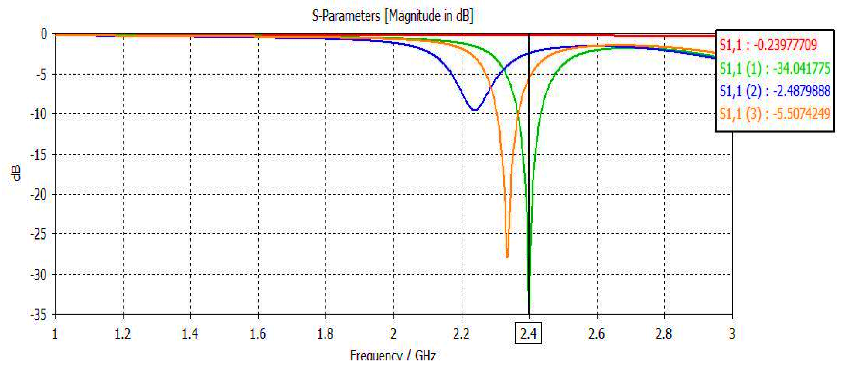
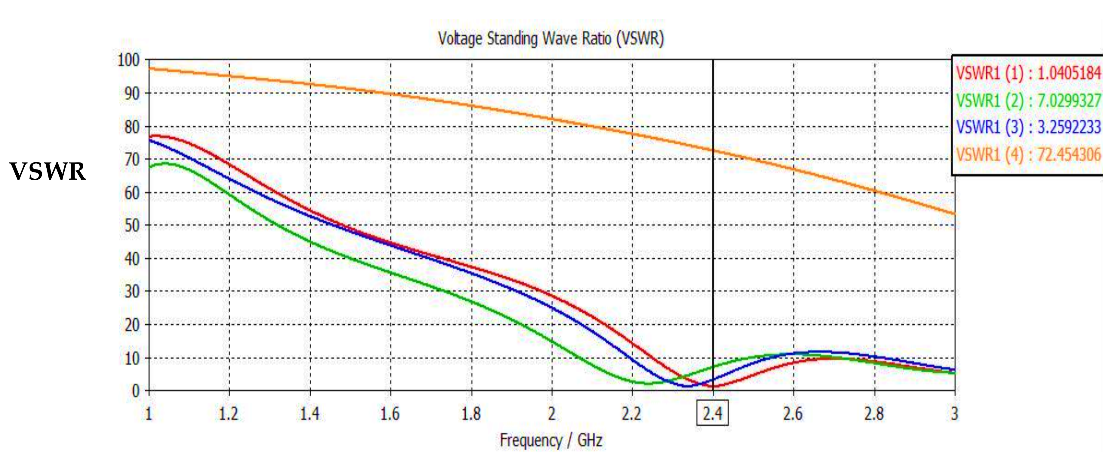
| Parameter | MROA | CSA | MCA | PSO |
| S_Parameter | −34.041775 | −0.23977709 | −2.4879888 | −5.5074249 |
| VSWR | 1.0405184 | 72.454306 | 3.2592233 | 7.0299327 |
Publisher’s Note: MDPI stays neutral with regard to jurisdictional claims in published maps and institutional affiliations. |
© 2021 by the authors. Licensee MDPI, Basel, Switzerland. This article is an open access article distributed under the terms and conditions of the Creative Commons Attribution (CC BY) license (https://creativecommons.org/licenses/by/4.0/).
Share and Cite
Hathal, H.M.; Ali, R.S.; Abdullah, A.S. A Novel Metaheuristic Moss-Rose-Inspired Algorithm with Engineering Applications. Electronics 2021, 10, 1877. https://doi.org/10.3390/electronics10161877
Hathal HM, Ali RS, Abdullah AS. A Novel Metaheuristic Moss-Rose-Inspired Algorithm with Engineering Applications. Electronics. 2021; 10(16):1877. https://doi.org/10.3390/electronics10161877
Chicago/Turabian StyleHathal, Hussein M., Ramzy S. Ali, and Abdulkareem S. Abdullah. 2021. "A Novel Metaheuristic Moss-Rose-Inspired Algorithm with Engineering Applications" Electronics 10, no. 16: 1877. https://doi.org/10.3390/electronics10161877
APA StyleHathal, H. M., Ali, R. S., & Abdullah, A. S. (2021). A Novel Metaheuristic Moss-Rose-Inspired Algorithm with Engineering Applications. Electronics, 10(16), 1877. https://doi.org/10.3390/electronics10161877