Concrete Cracks Detection and Monitoring Using Deep Learning-Based Multiresolution Analysis

Abstract

In this paper, we propose a new methodology for crack detection and monitoring in concrete structures. This approach is based on a multiresolution analysis of a sample or a specimen of concrete material subjected to several types of solicitation. The image obtained by ultrasonic investigation and processed by a customized wavelet is analyzed at various scales in order to detect internal cracks and crack initiation. The ultimate objective of this work is to propose an automatic crack type identification scheme based on convolutional neural networks (CNN). In this context, crack propagation can be monitored without access to the concrete surface and the goal is to detect cracks before they are visible. This is achieved through the combination of two major data analysis tools which are wavelets and deep learning. This original procedure is shown to yield a high accuracy close to 90%. In order to evaluate the performance of the proposed CNN architectures, we also used an open access database, SDNET2018, for the automatic detection of external cracks.

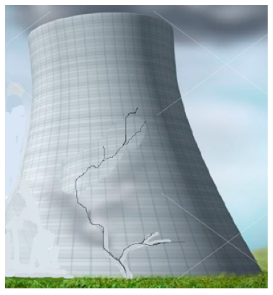
1. Introduction

Concrete is one of the most widely used man-made materials in the world. Nevertheless, the search for simple, effective and low-cost techniques to optimize the performance of concrete and to control its structural behavior is a real challenge we must meet. In the interests of safety and economy [1,2], methods for predicting the performance of concrete structures have become necessary, especially in developing countries. Among the causes of concrete damage, mechanical overloading appears to be the most common. Micro-cracks (see, for example, Figure 1a) can be caused by mechanical stresses, often local. These micro-cracks can evolve and propagate in the structure and cause irreversible damage [3]. For this reason, monitoring of cracks is essential. Operationally, this monitoring is usually performed by regularly evaluating the beginnings of surface cracks by optical means or extensometers.

However, with these conventional methods, internal damage is not detectable, hence the increased use of non-destructive testing to detect cracks at an early stage.

Concrete is a mixture of four main materials: Portland cement, coarse aggregate, fine aggregate and water, and for industrial use, mineral and chemicals admixtures are added to accelerate or delay its grip and improve its performance [1,4]. The quantities of these elements are regulated for a quality required by the purpose of the structure’s construction, such as long span bridges (see Figure 1b), special underground structures (see Figure 1c), nuclear power plants (see Figure 2). An excess or a defect in the required quantity of one of the constituent elements, or an inappropriate vibration of the initial mixed elements causes defects such as segregation or premature cracks due to shrinkage of the concrete. Moreover, the presence of air bubbles causes discontinuities in the material (see Figure 1).

These defects affect the strength of concrete and its durability [3]. Exposed to aggressive environments or temperature variations, visible and non-visible defects appear, and the concrete’s quality and resistance decrease. Under compressive stress, this material behaves well, unlike tensile stresses which can cause substantial damage. In a concrete specimen subjected to compressive stress, the constraints are concentrated on rigid elements with an appreciable modulus of elasticity. Since this material is heterogeneous, an external load creates a complex state within it and a concentration of stresses around air voids [4].

Non Destructive Testing (NDT) [5] is a set of methods that are commonly used to characterize the state of integrity of structures, without degrading them, either during production (e.g., during construction of structures or buildings) or during use or service [6,7]. The development of NDT methods began in the 1960s to meet the demands of sectors such as nuclear energy, aeronautics and space. NDT gradually widened its field of application, moving from the strict field of detection, recognition and dimensioning of localized defects to the evaluation of the intrinsic characteristics of materials. The notion of defect (or fault) is defined according to the use that will be made of the product (satisfaction of the final customer).

In the case of early detection of concrete cracks and especially in case of internal damage, NDT is the ideal tool not only for the detection of cracks but also for monitoring their propagation [8,9].

The main objective of this study is to propose an original technique for the detection of structural cracks in concrete by using an ultrasonic non-destructive testing system to scan the concrete coupled with an evaluation methodology based on multiresolution analysis and deep learning.

• Wavelet-based multiresolution analysis is a tool that allows analysis at multiple scales or resolutions and mimics the effect of a microscope [10];
• Deep learning is a type of artificial intelligence where the machine is able to learn by itself, as opposed to programming where it simply executes predetermined rules. Deep learning is based on neural networks with several layers of hidden neurons, each receiving and interpreting information from the previous layer. The most powerful deep learning architecture is called convolutional neural networks (CNN). CNN is broadly composed of three types of layers: convolution, pooling and fully connected layers. CNN receive input images, automatically detect and extract the features of each of them. This is done by the first two layers, i.e. convolution and pooling. The third is a fully connected layer that transforms the extracted features into a final output, such as classification. Moreover, the specific architecture of this network allows the extraction of features of different complexity, from basic or low level as edges, corners, texture to the most complex or high level as patterns, objects. The automatic extraction and prioritization of features, which are adapted to the given problem, is one of the strengths of CNN. In 2012, at the annual ILSVRC (ImageNet Large Scale Visual Recognition Challenge) computer vision competition, a new CNN-based Deep Learning algorithm, named AlexNet, broke all records [11]. CNN has since then been the best performing model for image classification. This is what motivated its use in our experiment.

The remainder of this paper is organized as follows.

Section 2 is devoted to the foundations of our approach.

• It presents and recalls NDT methods and techniques as well as the experimental set-up used;
• It introduces the main properties of the wavelet transform and the corresponding multiresolution analysis;
• It recalls the foundations of neural networks and CNN-based Deep Learning, and proposes the adopted architecture to build a classifier for detecting internal cracks from the obtained spatial-scale images.

Section 3 focuses on the implementation aspect and the analysis of the results.

Finally, Section 4 concludes this study.

2. Materials and Methods

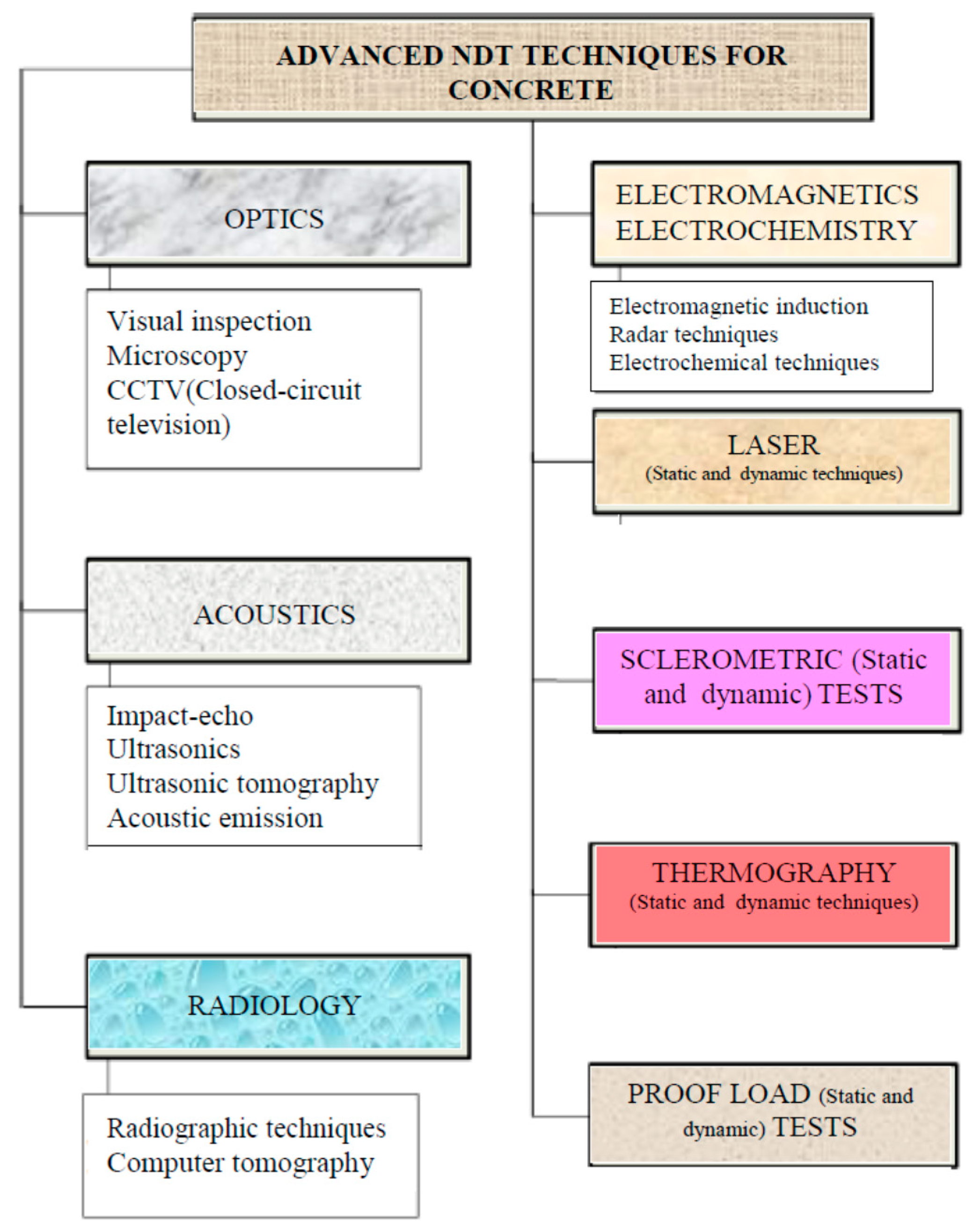
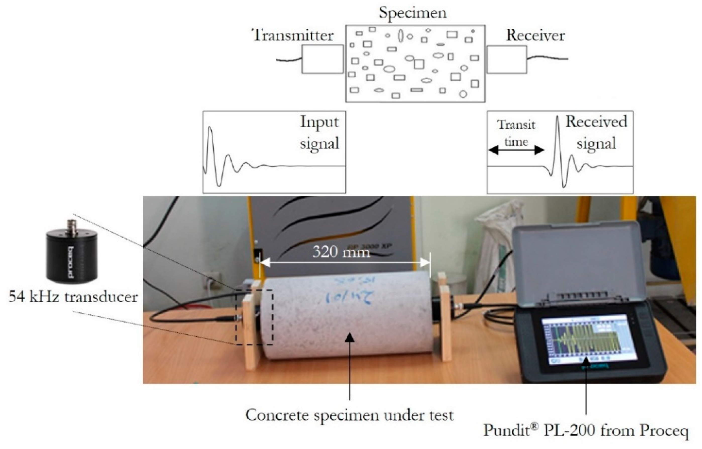
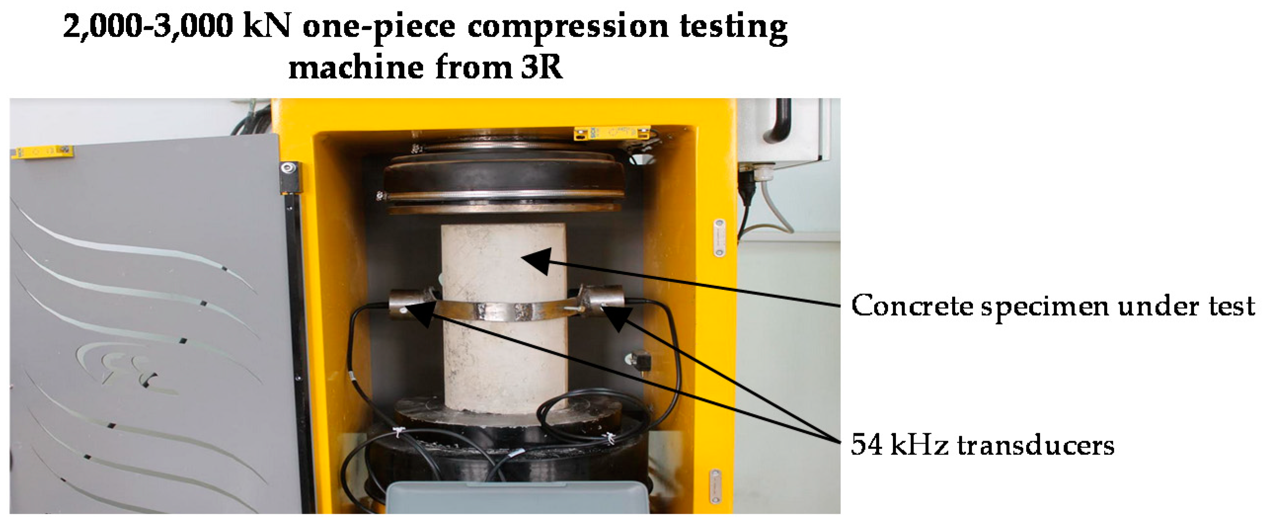
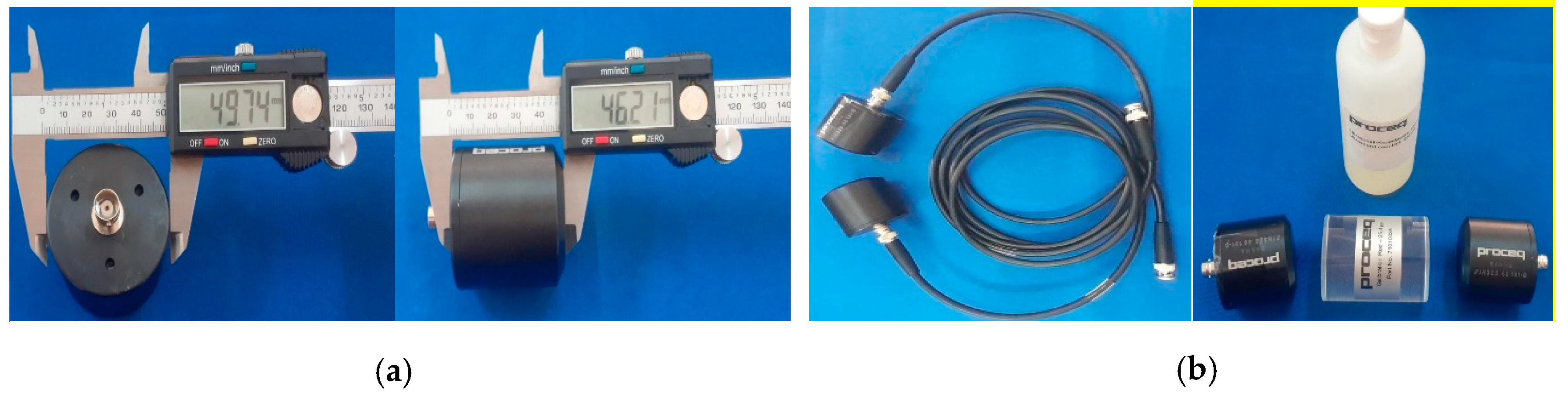
2.1. NDT Methods

The most commonly used NDT methods and techniques [12] are optical NDT [13], ultrasonic NDT [14], acoustic emission testing [15], radiographic NDT [16,17,18], eddy-current testing [19], electromagnetic NDT [20], laser systems [21], sclerometric [22] and thermographic [23] methods for evaluating the durability of concrete structures by contact and non-contact. Figure 3 shows the main NDT techniques for concrete structures.

In this study, the analysis of the ultrasonic wave propagation [24,25,26] is performed using 2 sensors located on opposite sides of the analyzed specimen (see Figure 4 and Figure 5).

Figure 4 and Figure 5 show the devices used experimentally to determine the presence or absence of cracks in concrete subjected to compression. The ultrasound device used is a Pundit L200 from the company Proceq. The press used is a 3R monobloc compression press with a capacity of 2000 kN to 3000 kN adapted to specific tests on concrete specimens of cylindrical shape. The test specimen is of standardized dimension, cylindrical in diameter 16 cm and height 32 cm. Its weight is 15 kg. The test specimen is over 90 days old. The charging speed is 0.05 Mpa/s. The signal transit time varies from 32.3 to 71.4 microseconds when the compressive force varies from 0 to 470 kN.

For our NDT experiments to determine cracks or defects in concrete, the ultrasonic pulse velocity varies from 3000 m/s (low quality) to 5000 m/s (high quality). For ordinary concrete, an average value of 3700 m/s (longitudinal wave) and 2500 m/s (shear wave) have been used for the computation of the wavelengths, the maximum aggregate size and the minimum lateral dimension test specimen. Figure 6 and

Table 1. Technical specifications of the sensors used in our NDT experiments.

Technology	Frequency	Wavelength	Maximum Grain Size	Bandwidth	Pulse Shape	Weight
P-wave transducer	54 kHz ± 5 kHz	68.5 mm	34 mm	<10 kHz	Square wave	287 g

give the specifications of the sensors used.

The originality of our work lies in the fact that we use, on the one hand, the ultrasound-based NDT method to identify possible cracks and, on the other hand, this method is combined with a multiresolution analysis based on wavelets to finely analyze cracks and their size at different scales, especially at the beginning of the concrete cracking process. The final objective is to automatically classify these cracks by deep learning and to enable their identification according to type.

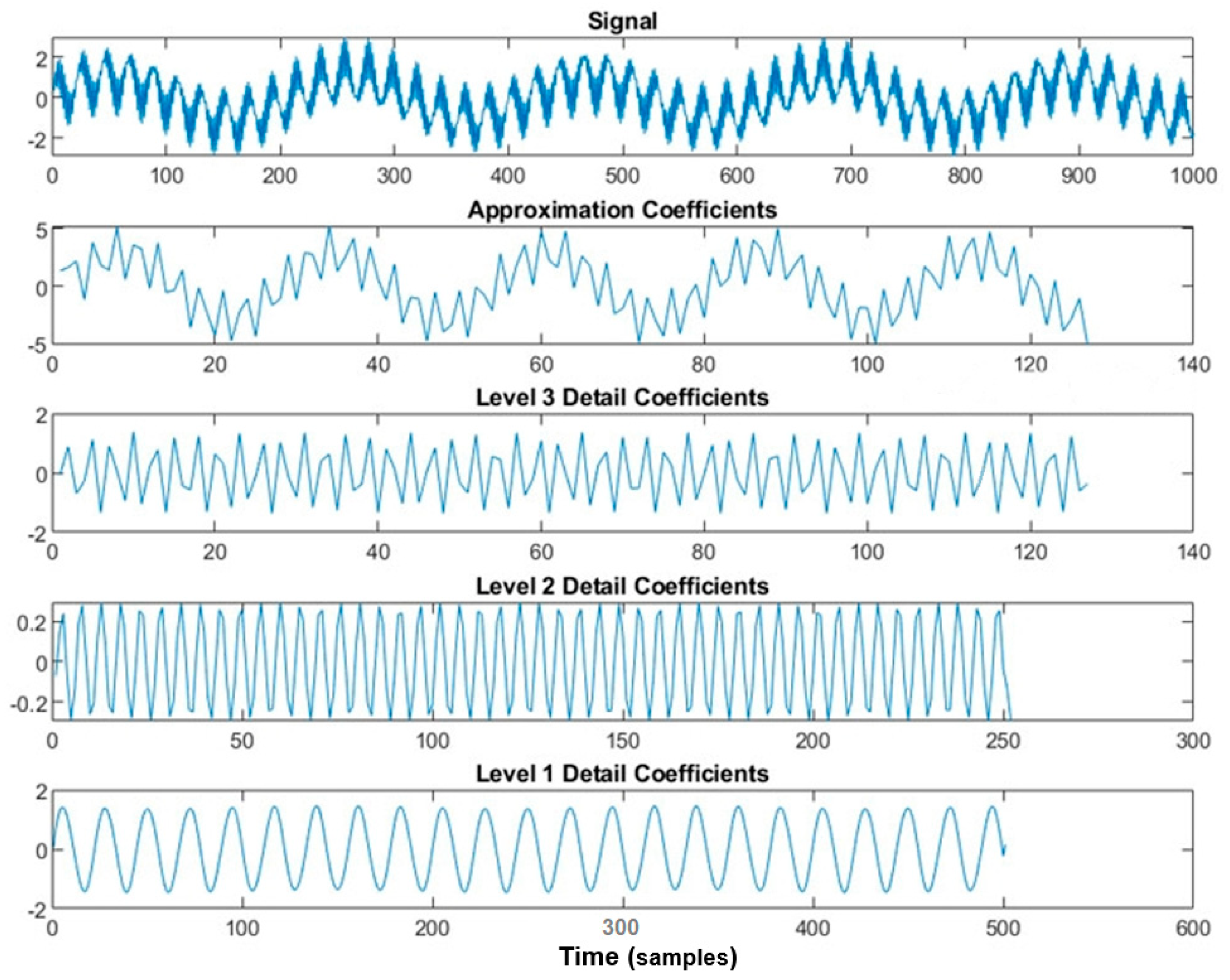
2.2. Multiresolution Analysis Based on Wavelets

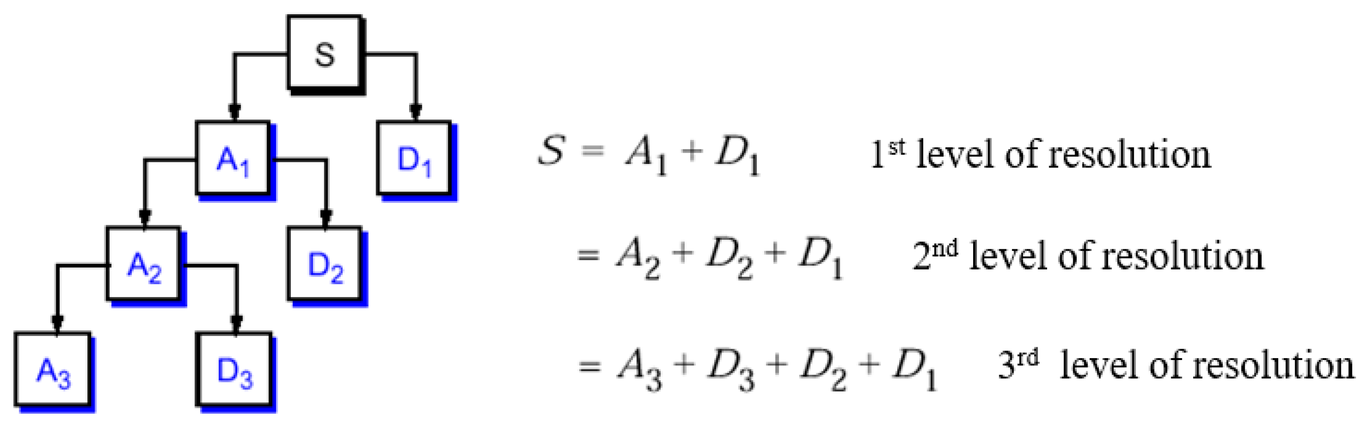
2.2.1. Concepts of Multiresolution Analysis

The idea of multiresolution analysis [10] of a signal is based on the fact that the signal is decomposed over a very wide range of scales, an operation that can be compared to a cartography. At each scale, the signal will be replaced by the most adequate approximation that can be drawn. By going from the coarsest scales to the finest scales, we get access to more and more precise representations of the given signal. The analysis is done by calculating what differs from one scale to another, in other words the details at a given resolution. This allows, by correcting a still rather coarse approximation, to reach a representation of better quality.

An acceptable representation of the data to be visualized should be hierarchical and should achieve the following objectives [10].

• Global view at an arbitrary resolution;
• Exact local view;
• Progressive transmission by network;
• Compression.

Moreover, the algorithms achieving these objectives should have a minimal average computational cost in time and space, typically $O\left(N\right)$ where $N$ is the size of the signal being analyzed. All these characteristics are fulfilled by the hierarchical data representation based on multiresolution wavelet transform analysis. These multiresolution analysis methods allow a signal representation at several resolution levels by storing the coarsest resolution level, as well as the errors between successive levels. This coding by successive errors, rather than by storing all the levels of resolution, explains the linear cost in space of multiresolution analysis algorithms. The errors are coded by the detail coefficients. Each of these coefficients is associated with a basis function, called a wavelet because of its oscillating behavior, and its locality. The applications that interest us in the context of visualization result from the selection of certain detail coefficients - and the deletion of others - after the analysis, and before the synthesis. This selection is based on the orthogonality and locality properties of the wavelet basis.

The orthogonality properties link the error caused by the suppression of detail coefficients with the value of these coefficients: the error will be small if low magnitude coefficients are suppressed. The locality properties allow to specify the area influenced by the suppression of a detail coefficient. Thus to obtain a global view at an arbitrary resolution, we can select the desired percentage of the most significant detail coefficients (i.e., the largest in absolute value). Compression is based on the same principle. Progressive transmission is optimized by transmitting the detail coefficients in decreasing order of magnitude. Finally, an exact local view is obtained by selecting all the detail coefficients whose area of influence intersects the region to be visualized. These properties explain why multiresolution analysis has already been successfully used in visualization, for example for the visualization of volumetric medical data or oceanographic data. In this study, multiresolution analysis is used for the visualization of cracks in concrete.

Researchers, engineers and practitioners in various fields such as multimedia [27], telecommunications [28,29,30], medicine and biology [7,31,32], crack tracking and fracture detection [8,9,33,34,35], fluid mechanics [36] thermodynamics [37], astrophysics [38], finance [39,40] deal daily with data at various scales of analysis, for of classification, segmentation, detection, denoising [41], compression, synthesis or reconstruction, etc. However, wavelet transform-based multiresolution analysis imposes restrictions that prevent certain types of visualizations, or even prohibit the visualization of certain types of data. For example, the first generation wavelet analysis is not able to produce an analysis according to all the orientations of an image as only the horizontal, vertical and diagonal components are taken into account. Hence the emergence of new paradigms called 2nd or 3rd generation wavelets such as ridgelets [42], curvelets [43], contourlets [44], bandelets [45], etc.

Figure 7 summarizes the principle of multiresolution analysis for three levels of resolution based on wavelets. The signal S is first decomposed at the 1st resolution level into an approximation A₁ and a detail D₁, then at the 2nd resolution level, approximation A₁ is decomposed into an approximation A₂ and a detail D₂, and finally at the 3rd resolution level, approximation A₂ is in turn decomposed into an approximation A₃ and a detail D₃.

The signal thus analyzed can be written as follows:

$$S=A_3+D_3+D_2+D_1$$

(1)

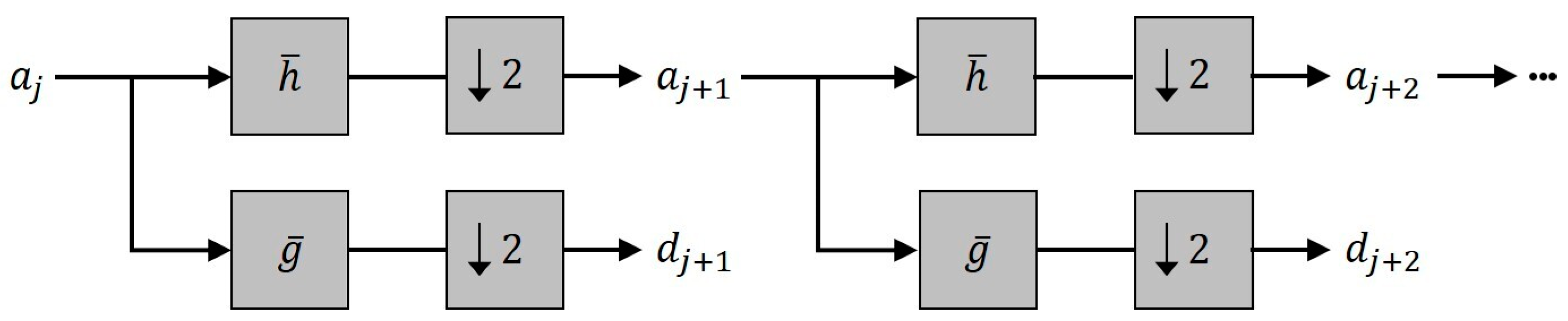
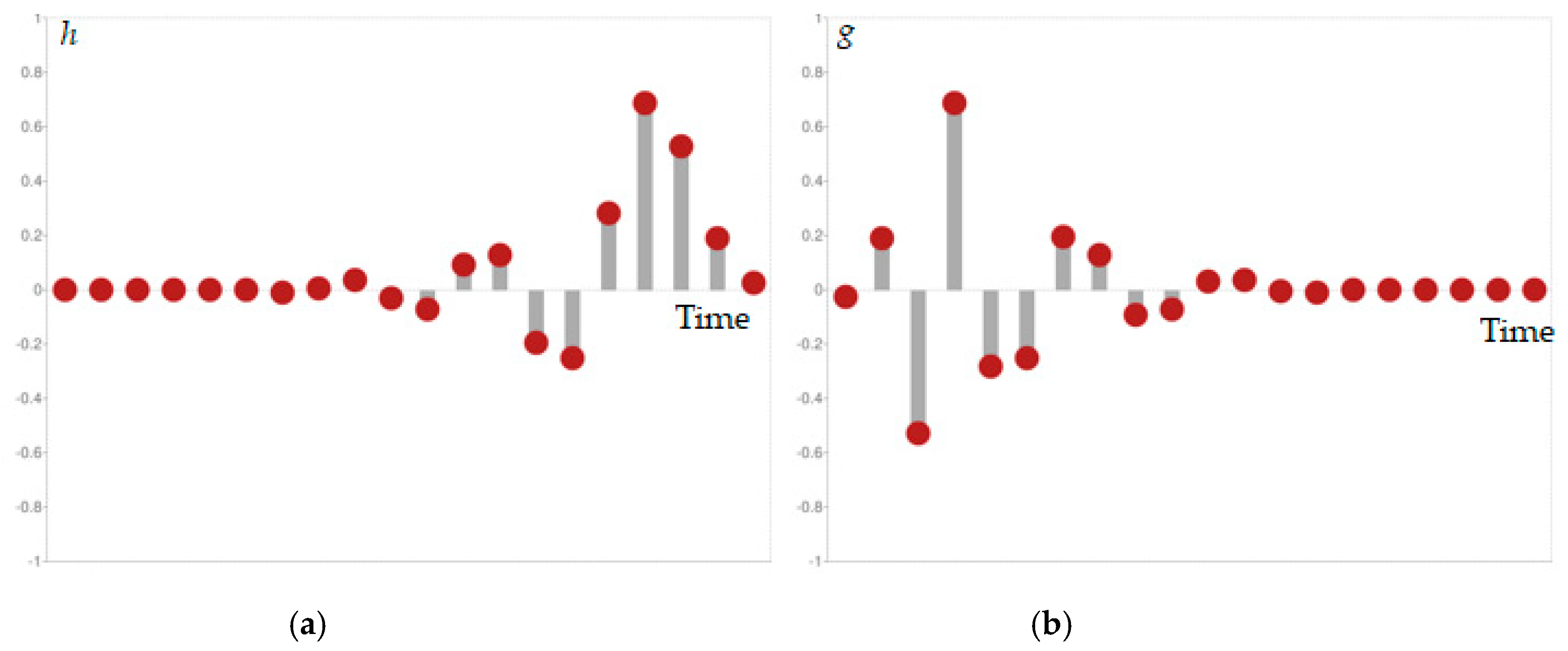
2.2.2. Wavelet Transform and Its Discrete Version

In this section, we will make the link between wavelet transform and multiresolution analysis.

The chosen wavelet, denoted ψ(t), must satisfy the following property:

$$\underset{ℝ}{{\displaystyle \int }}{t}^p\psi \left(t\right)dt=0, \forall 0\le p<n$$

(2)

where n controls the number of oscillations of ψ(t).

This relation means that ψ(t) “kills” polynomials of degree $p$ for $p<n.$ The wavelet transform $W_X\left(u,s\right)$ of a signal X at time u and scale s is defined by (3).

$$W_X\left(u,s\right)=\underset{ℝ}{{\displaystyle \int }}X\left(t\right){\psi }^{*}\left(\frac{t-u}{s}\right)dt$$

(3)

where ${\psi }^{*}$denotes the complex conjugate of $\psi$.

Expressions (2) and (3) show that $W_X\left(u,s\right)$ is unaffected by a signal that is represented by a polynomial of degree smaller than $n$. In contrast, $W_X\left(u,s\right)$is sensitive to irregular variations. This characteristic of the wavelet transform has a major importance in singularity detection, especially in crack detection and monitoring.

The discrete wavelet transform (DWT) is given by Equation (4).

$$d_X\left(j,k\right)=W_X\left(u=2^{-j}k,s=2^{-j}\right) \left(j,k\right)\in {\mathbb{Z}}^2$$

(4)

It is obvious that to avoid redundancy, the family ${\left\{{\psi }_{j,k}\right\}}_{\left(j,k\right)\in Z^2}$ must be an orthonormal basis.

This property of the wavelet makes it possible to obtain a fast wavelet transform.

The fast wavelet transformation is calculated by a cascade of low-pass filtering by $h$ and high-pass filtering by $g$ followed by a down sampling (see Figure 5).

In Figure 8, $a_{j }$(or $a_X\left(j,k\right),$ where $k$ represents time) and $d_{j }$(or $d_X\left(j,k\right)$) are called respectively approximation coefficients and wavelet coefficients (or details) of the signal at level $j$. Moreover, the symbol represents the decimation (down sampling) symbolizing the conservation of one sample out of two.

In Figure 8, the mirror low-pass filter is $\overline{h}\left(k\right)=h\left(-k\right)$ and mirror high-pass filter $\overline{g}\left(k\right)=g\left(-k\right)$ are shown.

These two impulse responses [10] are linked by $g\left(k\right)={\left(-1\right)}^{k}h\left(1-k\right)$ whose coefficients are obtained directly from the chosen wavelet ψ.

Figure 8 clearly shows that in reality the fast (or digital) wavelet transform is performed iteratively, and the calculation is performed at each resolution. For example, if we are interested in analyzing the signal with 5 resolutions, in this case the basic pattern consisting of low-pass filtering followed by decimation, and high-pass filtering followed by decimation will be repeated five times.

This approach shows the link between the wavelet transform and multiresolution analysis.

The example in Figure 9 is intended to show the original signal analyzed at 3 resolutions.

In Figure 9, it should be noted that the original signal has 1000 samples while the detail (and approximation) signals have been decimated by a factor of 2 at each level of resolution. Hence, after 3 levels of resolution, from a signal of 1000 samples, one arrives at the approximation A₃ and the detail D₃ which each have only 125 samples.

2.2.3. Scalogram of the Received Ultrasound Signal

In this work, the scalogram of the investigative ultrasound signal will be used to determine and analyze cracks in concrete. We can define the scalogram of the signal $x\left(t\right)$ by

$$S_X\left(j,k\right)={\left|d_X\left(j,k\right)\right|}^2 \forall \left(j,k\right)\in \mathbb{Z}\times \mathbb{Z}$$

(5)

The non-destructive testing (NDT) of the concrete sample is carried out by emitting an ultrasonic signal, which passes through the concrete sample. Thus, the received ultrasonic signal undergoes a multi-resolution analysis via a discrete wavelet transform (DWT). A scalogram is constructed from this transformed ultrasound signal by taking the square modulus of the DWT.

This scalogram will be assimilated to a space-scale image allowing to localize the crack in space and at each resolution. The scalogram image will be used as an input to the CNN architecture which will automatically detect a defect or a possible internal crack.

Figure 10 shows the scalogram of a signal representing the initialization of a crack materialized by intense energy. This fracture also propagates, even if in a weaker way, to other scales which can cause in the long term to a rupture.

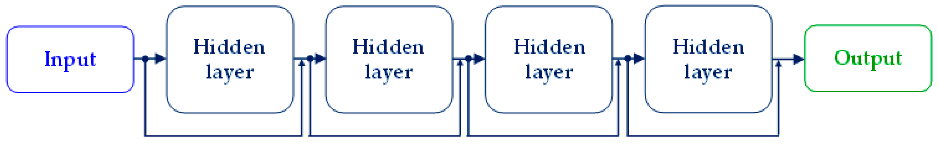
2.3. From Neurons to CNN and Deep Learning: Basic Concepts

In this section relating to artificial intelligence based on neural networks, we will recall the main functions used in our experiment of automatic detection of cracks in concrete structures.

2.3.1. Fundamental Concepts of Neural Networks Used in Our Experiment: A Brief Review

An artificial neural network is an intelligent computer system, hardware and/or software, that automatically processes information for application areas in system identification and control (vehicle control, trajectory prediction, process control, natural resource management), general gaming, pattern recognition (radar systems, face recognition, signal classification, 3D reconstruction, object recognition, speech recognition, etc.), medical diagnosis, finance, data mining, visualization, machine translation, social network filtering, spam filtering, etc. It consists of a set of interconnected neurons, each with digital inputs and outputs. The output of an artificial neuron depends on the weighted sum of its input values and an activation function. An artificial neural network has an input layer (the data), an output layer (the results), and can have one or more intermediate layers called hidden layers.

This basic neuron model can be defined by the following operations:

• The combination function: in the initial model, it is simply a weighted sum of the input values.
• The activation function: this is what will determine the output value. It is based on the result of the combination function, as well as on a pre-set threshold. It can, for example, be a simple “staircase function”, which returns 0 if the weighted sum of the inputs is lower than the threshold value, and 1 otherwise.

Finally, the result is sent to the output of the neuron. This information can then be transmitted to several other neurons, via branches with associated weights.

Deep learning is so called because of the structure of the neural network it uses which consists of a layered configuration of neurons: the higher the number of hidden layers, the deeper the network. The first layer receives the input data, and the last one provides the network output. Between the two are the hidden layers.

Each neuron is associated with a set of adjustable parameters that can be adapted by training. The weights associated with a neuron $i$ with $n$ inputs are represented by a vector of weights of dimension $n$: $w_i\in {ℝ}^n$.

The representation and processing power of these neural networks depends on the functions used at the level of the neurons, but also on the architecture of the network (number of neurons and type of connection between them).

During the training phase, the neural network modifies the weights of the inputs of each neuron. This consists essentially of adjusting the weights in a way that allows the network to correctly classify all the examples of the training set. As this is basically an optimization problem, a variety of methods can be used to determine these weights.

Neural networks can be used to perform diagnosis. In this context, we assume that the classes of recognizable diagnoses are known. Making a diagnosis consists in determining to which class a particular situation belongs (crack/non-crack).

In the following, we will discuss two points to be taken into account in our work:

• Overfitting

The overfitting issue is mainly related to the inadequate dimensioning of an architecture: For example, the number of hidden layers and/or the number of hidden neurons per layer is too high. This phenomenon reduces the generalization capacity of the network.

In practice, if the number of hidden neurons is too low, the network has too few adjustable parameters (it is “under-parameterized”) and cannot capture, during its training phase, all the dependencies between the input vectors (stimuli) that are presented to it and the different desired outputs (targets). Conversely, if the number of hidden neurons is too large, the number of adjustable parameters of the network is also too important. The network becomes “overparameterized” and can reach several hundred parameters and a few dozen layers. It then becomes possible, during the training phase, either to model unnecessarily certain relations which are only the result of statistical fluctuations specific to the training examples, rather than fundamental dependence relations, or to fall in a scenario of overfitting. This phenomenon prevents the trained network from correctly processing the inputs that are later presented to it [46].

2.

Properties of input data

It is imperative that the network inputs have a mean close to zero and a variance close to one. This is why it is necessary to normalize them. Moreover, the amplitude of these inputs must not be too large in order not to saturate any neuron, which would slow down its convergence and, in fine, block the training phase of the network.

In the context of this work, the objective is to classify the sample defect as crack or non-crack. The network calculates a probability value $p$ from its inputs and the crack/non-crack result will be represented by the probability values p and $1-p$ respectively.

These final probabilities are calculated by the last layer and the loss function calculate the classification error. The best performing loss function is based on cross-entropy [47], and this is what we have adopted in this work. The optimization of this loss function by stochastic gradient descent [48] allows the learning of the weights in the different layers by backpropagation of the gradient. The parameters that minimize the regularized loss function are progressively calculated for each layer, starting from the end of the network.

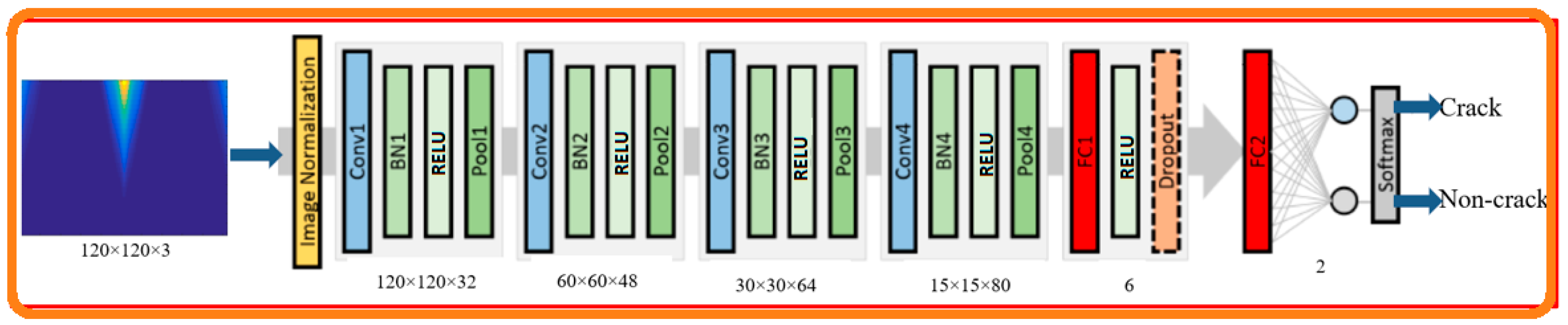
2.3.2. CNN and Deep Learning Principle

Artificial intelligence based on neural networks has seen an extraordinary resurgence of interest after the resounding success at the 2012 ImageNet competition of a new deep learning architecture-AlexNet. This new model is based on convolutional neural networks (CNNs).

CNNs process input images where they extract their features and the last layer provides the “voting” of the classes (in our experiment, there are only 2 classes: crack/noncrack) that we are after. As for any neural network, its parameters are optimized by minimizing a loss function. Unlike other machine learning methods, CNNs have the particularity of using convolution to automatically detect and extract relevant features from the image. As can be seen in Figure 11, this first operation (Conv) is followed by 3 other operations (BN, RELU, and Pool), then the process starts again at the 2nd stage of the architecture and so on. The last stage of the CNN is dedicated to the classification [49,50,51,52] and gives as output probabilities related to the problem treated. In our case, the classification is binary: crack with probability $p$ versus non-crack with probability $1-p$.

There are in total seven main operations in the CNN architecture as illustrated in Figure 11.

Figure 11 shows a CNN architecture adapted to our concrete crack detection problem. This consists of 4 CONV layers, 4 BN layers, 4 RELU layers and 4 Pool layers, followed by a FC, RELU and Dropout layers. Finally, an FC layer decides, via Softmax activation, the final classification of the image into crack or non-crack. The numbers mentioned refer to the output data size of each block in the network.

These operations are described below:

CONV: The convolution layer is the fundamental element of the CNN, and it is always the first block of the network. The main objective of this convolution is to find the features by sliding a filter along the image according to a predetermined stride. This filter is initialized either randomly, or by a priori knowledge, or by transfer learning as explained later in this section. These filters will be updated during the optimization process when training. The results of this filtering represent the desired features. Four important hyperparameters allow to dimension the output volume of the convolution layer [53]:

• Number of convolution kernels or filters or feature detectors. It’s a power of 2 between $2^5$ and $2^{10}$. The use of a large number of filters results in a more powerful model, i.e. it can detect and extract the maximum number of relevant features, but there is a risk of overfitting due to the increase in the number of parameters.
• Filter size. Usually $3\times 3$ filters are used, but $5\times 5$ or $7\times 7$ are also used depending on the application. Keep in mind that these filters are 3D and also have a depth dimension, but since the depth of a filter at a given layer is equal to the depth of its input, it will be omitted.
• Stride controls the overlap of the receptive fields. The smaller the stride, the more the receptive fields overlap and the larger the output volume. This is in fact the sliding step of the filter.
• Zero-padding is sometimes convenient for putting zeros on the edge of the input volume. The size of this zero-padding is the third hyperparameter. This padding allows to control the spatial dimension of the output layer volume.

BN: Batch Normalization consists in normalizing (zero mean and unity variance) the inputs (or the activation of the previous layer) in order to speed up the training step and reduce the generalization error.

RELU: Rectified Linear Unit is the non-linear operation. Its role is to cancel the negative values in input.

Pool: (Max)Pooling or subsampling is an operation to reduce the size of images. Several possibilities of pooling exist, in our case, this operation is reduced to keeping only the maximum value in each patch of each feature map of size $2\times 2$ or $3\times 3$. The results are down sampled or pooled feature maps that highlight the most present feature in the patch. The objective of this operation is to reduce the number of parameters and therefore reduce the computational burden. Such an approach improves the performance of the network and prevents overfitting.

FC: Fully Connected layer is the last layer in any neural network. The fully connected layer is applied to a previously flattened input where each input is connected to all neurons. Such a layer is used to optimize objectives such as class scores. In our experiments, the image that has undergone a pooling operation will be followed by a flattening, i.e., putting the lines of the image one after the other to obtain a columnar “image”.

Dropout. Dropout method is used in CNN to randomly “deactivating” neuron outputs (with a predefined probability, e.g., 0.5 for the hidden layers and 0.8 for the input layer) during the training phase. This amounts to simulating a set of different models (bagging) and training them jointly (although none of them is trained end-to-end). As each neuron is possibly inactive during a learning iteration, this forces each unit to learn independently of the others. Dropout is therefore a technique that is designed to prevent overfitting.

Softmax. The softmax step can be seen as a generalization of the logistic function which takes as argument a vector of scores $x\in {ℝ}^n$ and which returns a vector of probabilities $p\in {ℝ}^n$ through a softmax function at the end of the architecture. It is defined as follows:

$$p=\left(\begin{array}{c}{p}_1\\ ⋮\\ p_n\end{array}\right) où p_i=\frac{e^{x_i}}{{{\displaystyle \sum }}_{j=1}^n{e}^{x_j}}$$

(6)

In our work, Softmax is the final activation function of our neural network used to normalize the output of the network to a probability distribution over the predicted output classes.

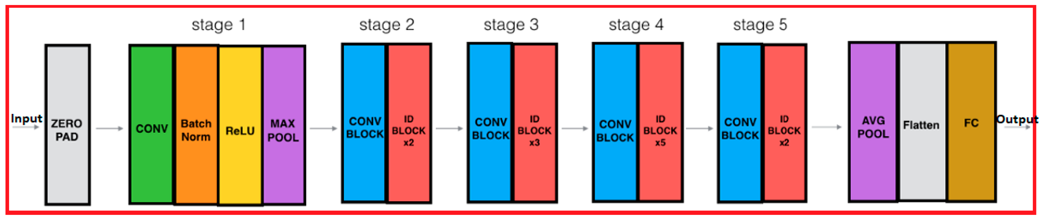
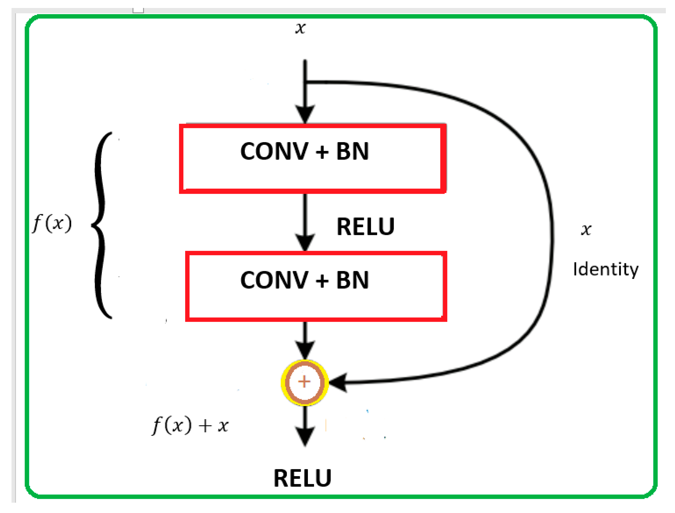
2.3.3. Residual Network Principle

In CNN, the depth of the network, i.e., the succession of layers in the network, allows the extraction of features of different levels of complexity, from basic or low-level features such as edges, corners, texture to the most complex or high-level features such as patterns, objects, etc.

However, He et al. [54] have shown that a significant increase in the number of layers does not necessarily lead to better performance. They show, using the CIFAR-10 and ImageNet datasets, that a 56-layer network gives a higher error than a 20-layer network. This highlighted that the deeper network has a higher training error, and thus test error. These authors show that the degradation of training accuracy is not due to overfitting, but indicates that not all systems are similarly easy to optimize.

He et al. address the degradation problem by introducing a deep residual learning framework called ResNet. Instead of hoping each few stacked layers directly fit a desired underlying mapping, they explicitly let these layers fit a residual mapping.

Formally, denoting the desired underlying mapping as $H\left(x\right)$, they let the stacked nonlinear layers fit another mapping of $f\left(x\right)=H\left(x\right)-x$. The original mapping is recast into $f\left(x\right)+x$. He et al., hypothesize that it is easier to optimize the residual mapping than to optimize the original, unreferenced mapping. To the extreme, if an identity mapping were optimal, it would be easier to push the residual to zero than to fit an identity mapping by a stack of nonlinear layers.

The formulation of $f\left(x\right)+x$ can be realized by feedforward neural networks with “shortcut connections” (see Figure 12). Shortcut connections are those skipping one or more layers.

In Figure 12, the shortcut connections simply perform identity mapping, and their outputs are added to the outputs of the stacked layers. Identity shortcut connections add neither extra parameter nor computational complexity. The entire network can still be trained end-to-end by stochastic gradient descent with backpropagation, and can be easily implemented using common libraries (e.g., Caffe [55]) without modifying the solvers.

To illustrate this notion, consider the case where the weights and biases of an ordinary neural network are initialized to 0. Each layer starts with the “zero” function. In contrast, in the same situation, ResNet essentially starts with the identity function since the input is passed directly to the output—it learns what is left (residuals) after the identity function is added. Hence the name residual network or ResNet!

These deep residual networks can easily benefit from gains in accuracy due to a significantly increased depth that can exceed 1000 layers (see Figure 13), producing results that are significantly better than those of previously used networks.

Sometimes shortcut connections are not represented in a ResNet configuration to simplify it, because shortcuts do not always occur symmetrically between layers.

2.3.4. Transfer Learning Concept

Training deep convolutional neural network models on very large datasets can take days or even weeks. One way to shorten this process is to reuse pre-trained model weights that have been developed for standard computer vision reference datasets, such as ImageNet image recognition tasks. The best performing models can be downloaded and used directly, or integrated into a new model for computer vision problems.

Transfer learning involves using models trained on one problem as a starting point for a related problem.

Transfer learning is flexible, allowing pre-trained models to be used directly, as feature extraction preprocessing, and embedded in entirely new models.

Keras provides convenient access to many high-performance models on ImageNet image recognition tasks, such as ResNet.

In summary, the objective of transfer learning is to accelerate the training process by introducing knowledge gained by a neural network that has handled a similar problem. Such a use also avoids overfitting.

Nowadays, we can easily retrieve one from the Internet, especially from Deep Learning libraries. For our part, we use the ResNet50 architecture found in the Keras library in transfer learning.

3. Results and Discussion

3.1. The Proposed Methodology

Figure 14 shows an outline of the proposed methodology to automatically detect internal cracks in a concrete specimen via a combination of non-destructive testing (NDT), multiresoluution analysis and classification stages. As depicted in the figure, the methodology consists of 3 main steps, starting with the NDT of the concrete specimen which produces an ultrasonic signal that detects the presence of an internal defect. This signal then proceeds to step 2 and undergoes a multiresolution analysis via a discrete wavelet transform (DWT).

A scalogram is constructed from the transformed ultrasonic signal to provide a space-scale image allowing to localize the crack in space and at each resolution. The scalogram image is then fed into step 3 of the method consisting of the CNN block which extracts the relevant scalogram image features that identify the type of internal defect and eventually classifies it as a crack or a non-crack.

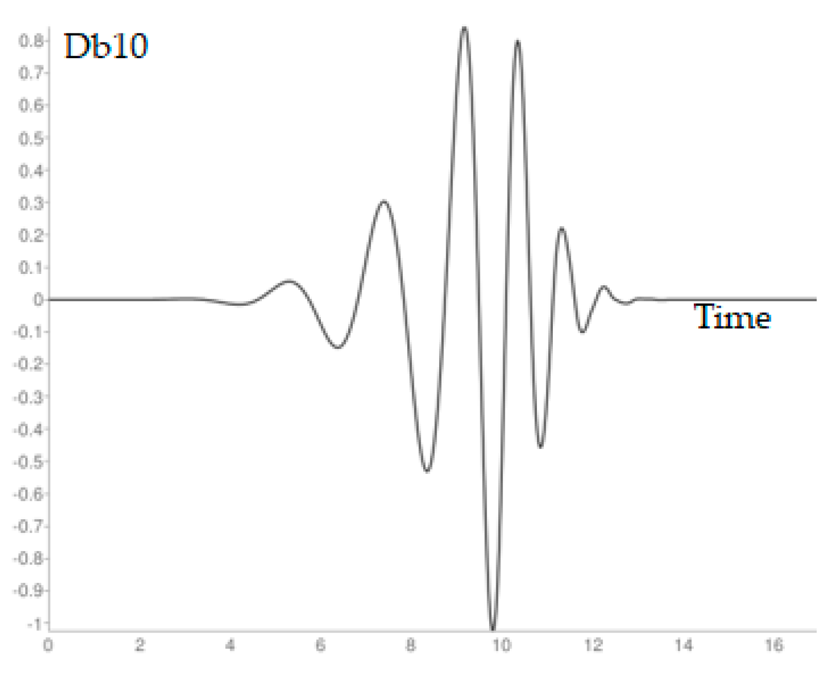
3.2. Wavelet Used for Multiresolution Analysis

We chose wavelet Daubechies10, noted Db10, to have the largest number of vanishing moments (see relation (2)), here $p=10$, for a given support width i.e., a number of coefficients of the corresponding filters equal to 20 [10].

In other words, this wavelet used for multiresolution analysis (or wavelet transform) perfectly analyzes the ultrasound signal since there will be a strong correlation between the analyzed signal and this wavelet. Moreover, visually, there is a strong resemblance between the received ultrasound signal and the Db10 wavelet (For comparison, see the ultrasonic signal in Figure 14).

This Daubechies wavelet, Db10, is shown in Figure 15. It is an orthogonal wavelet and widely used to detect signal discontinuities and cracks in structures, which justifies its use in our case.

Figure 16 shows the impulse responses $g$ and $h$ respectively of the low-pass and high-pass filters associated with Db10 (See also Figure 8 which shows the principle of multiresolution analysis using filters $g$ and $h$).

3.3. Metrics and Data Used

To achieve our goal of classifying cracked/non-cracked concrete images, it is necessary to use evaluation measures or metrics to assess the performance of our approach.

Accuracy is the ratio of the number of correctly predicted cracked and uncracked images to the total number of input images. Therefore, Accuracy is the number of correct predictions/total number of predictions, and it is defined by:

$$Accuracy=\frac{TP+TN}{TP+FP+TN+FN}$$

(7)

where TP (True Positive) and TN (True Negative) refer to images with and without cracks, which are correctly classified. FP (False Positive) and FN (False Negative) refer to images with and without cracks that are misclassified.

Precision or confidence is the number of images correctly assigned to the “cracks” class compared to the total number of images predicted as belonging to the “cracks” class (total predicted positive). Precision can be interpreted as an indicator of robustness. It is defined as:

$$Precision=\frac{TP}{TP+FP}$$

(8)

Recall or sensitivity is the number of images correctly assigned to the “crack” class compared to the total number of images belonging to the “crack” class (total true positive).

$$Recall=\frac{TP}{TP+FN}$$

(9)

$F_{\beta }$ score subtly combines precision and recall and corresponds to a weighted harmonic mean and is defined as:

$$F_{\beta }=\left(1+{\beta }^2\right)\frac{Precision\times Recall}{{\beta }^{2}Precision+Recall}$$

(10)

where β is a coefficient to arbitrate between precision and recall. If β is set to the value 1, it means that precision and recall have the same weight. This leads to the F₁ score defined as:

$$F_1=2\frac{Precision\times Recall}{Precision+Recall}=2\frac{TP}{2TP+FP+FN}$$

(11)

In this work, we propose two methodologies that depend on the nature of the concrete crack: internal or external. In this context, two sources of crack images were then used to develop an automatic detector of possible cracks.

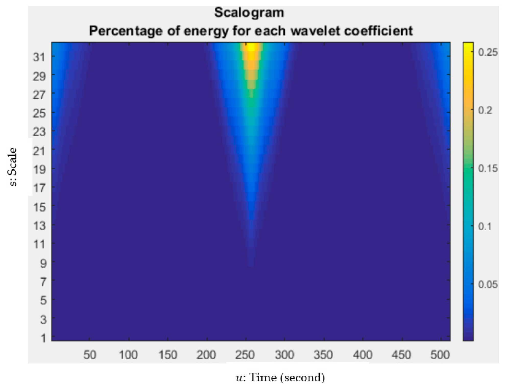
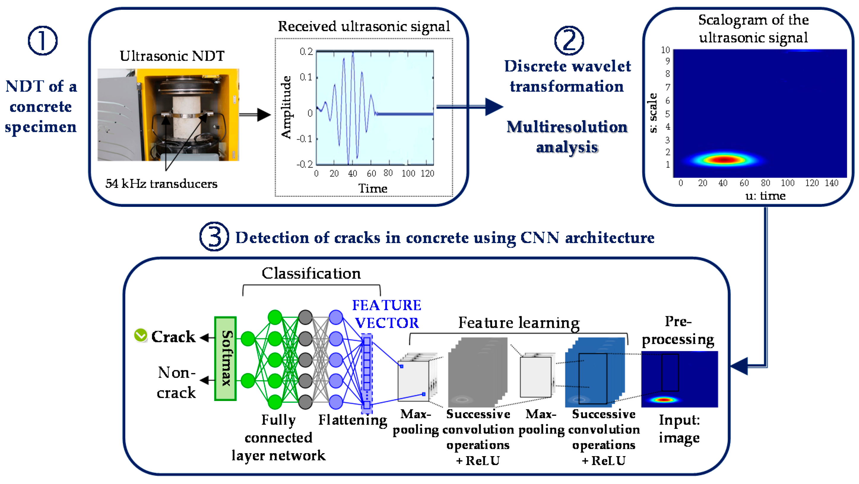
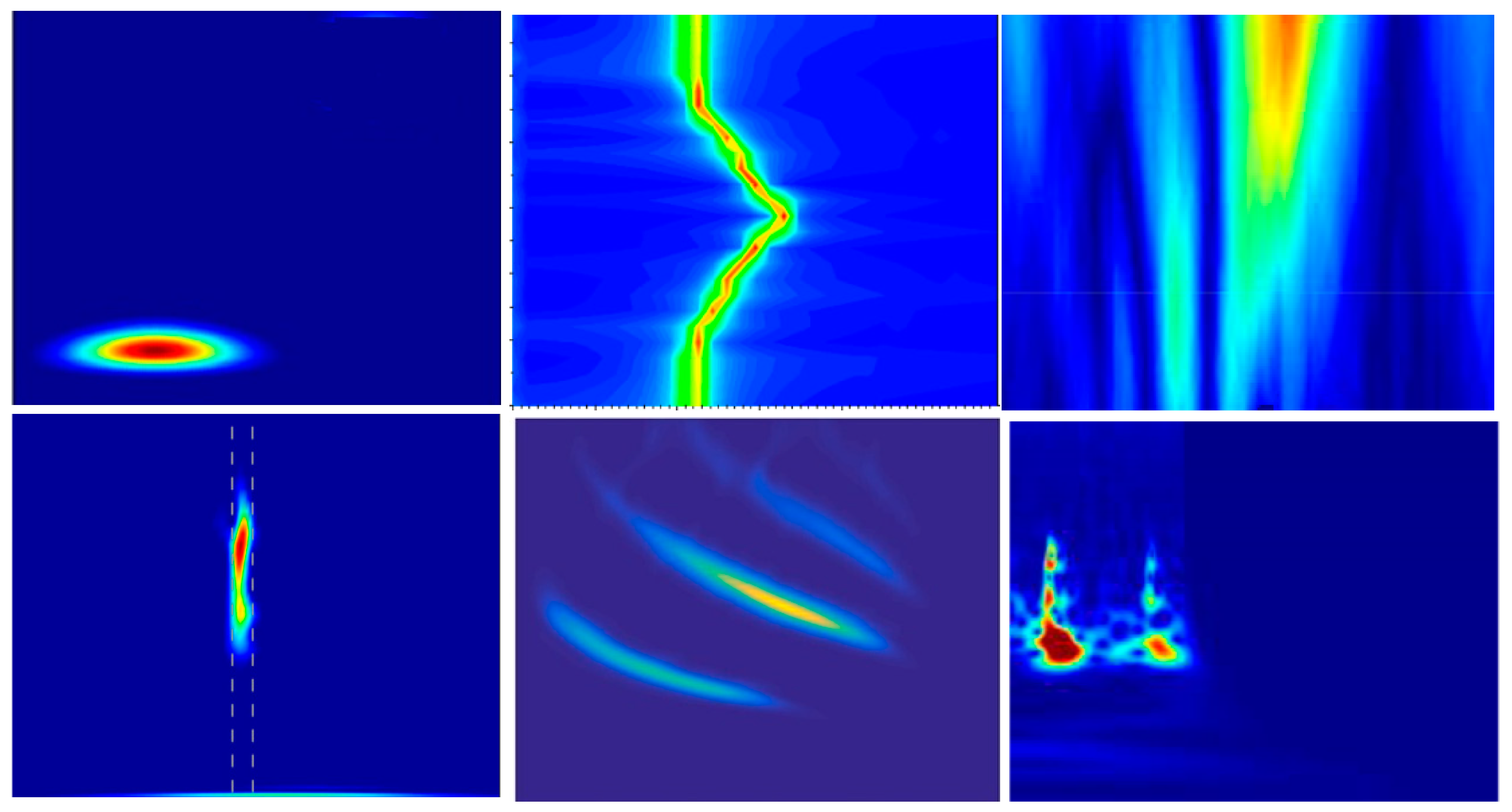
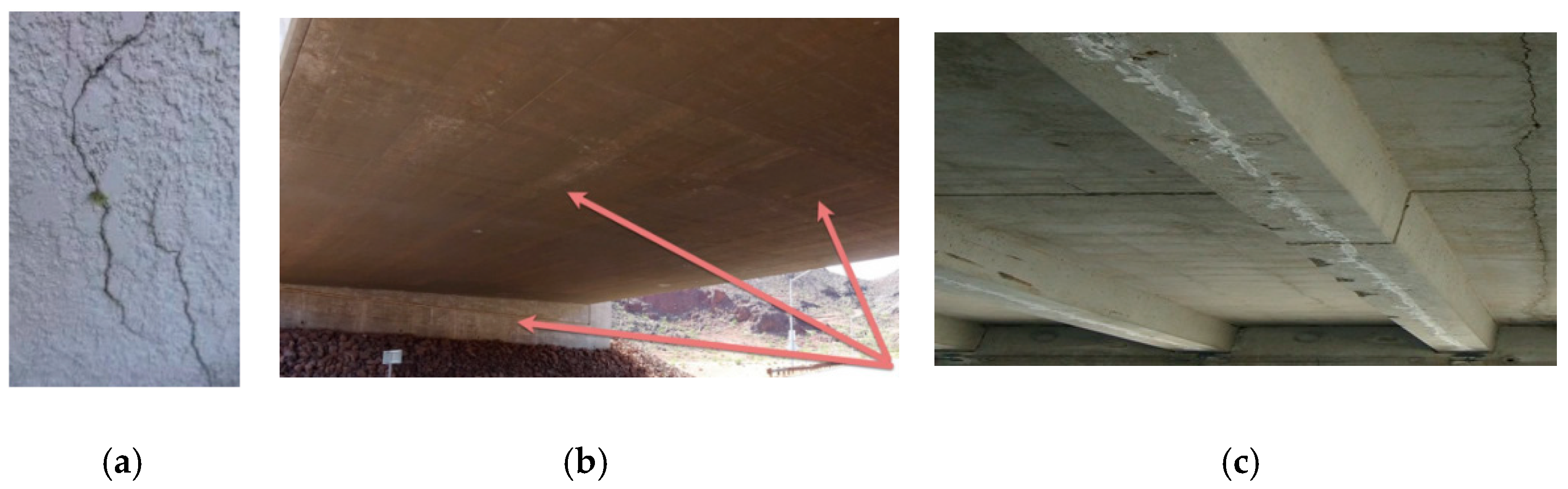
• The first source is derived from ultrasonic non-destructive testing images of internal cracks analyzed by wavelets. The multiresolution images are then classified into cracks/no cracks by deep learning.
  This original three-step approach is our main contribution.
  The procedure for obtaining these images is described in Section 3.1. In fact, these images are obtained by multiresolution analysis of the ultrasound signal that passed through the concrete specimen. As shown in Expression (5), it is the square modulus of the wavelet transform or scalogram of the received ultrasound signal.
  Figure 17 shows some examples of images or scalograms where the defect or crack is represented by a high intensity on the scalogram (yellow-red color).
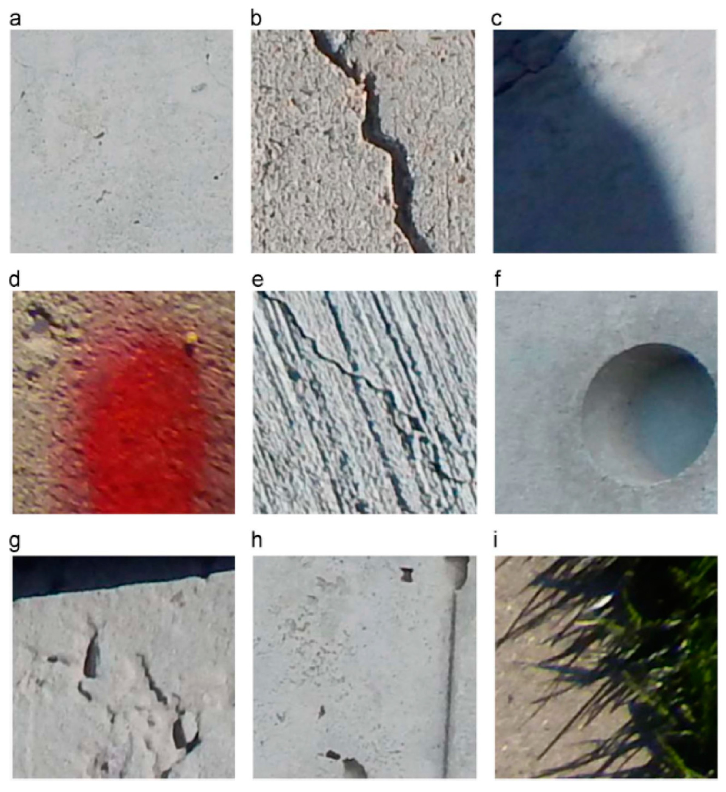
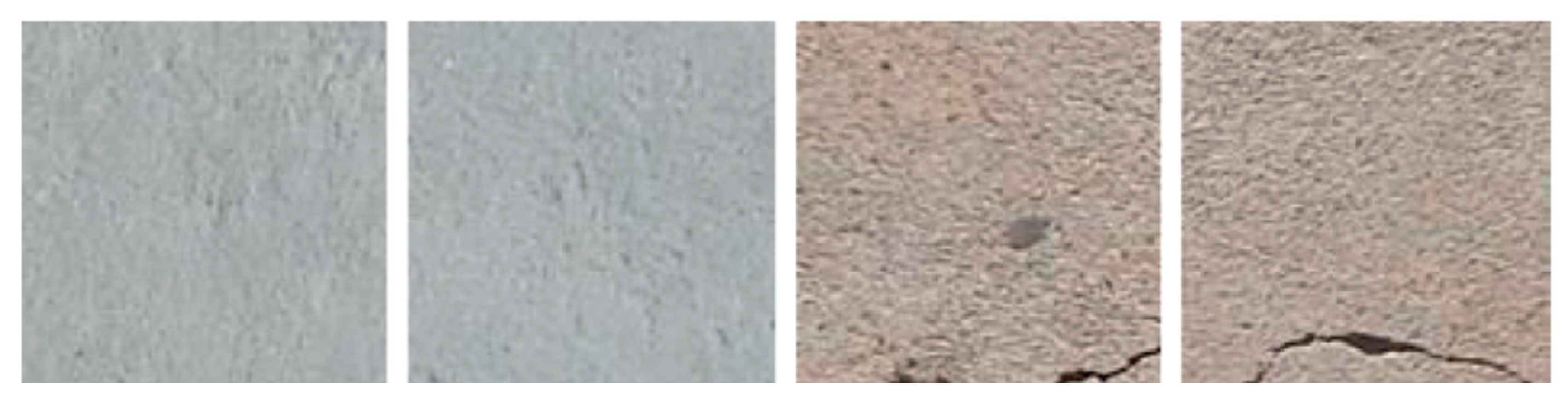
• The second source of images comes from SDNET2018 dataset [56].

SDNET2018 is an important database that can be used for crack detection in concrete structures. As shown in Figure 18 and Figure 19 several configurations are considered.

3.4. Implementation Aspect and Results Analysis

For the two data sources, i.e., on the one hand, the images obtained experimentally by NDT and multiresolution analysis, and on the other hand, the images of the SDNET2018 dataset, we selected 1000 images with cracks and 1000 images without cracks: 1600 images for the training phase and 400 images for the test phase. The size of each image is 256 $\times$ 256 pixels RGB.

For the SDNET2018 dataset, these are images of concrete bridges and it was possible to introduce various changes, such as lighting conditions and crack surface texture, to test and evaluate the generalization of the model.

All experiments are run on TensorBook equipped with a Super GPU 2080. It is equipped with Lambda Stack which is a software tool to manage installations of TensorFlow, Keras, PyTorch, Caffe, Caffe 2, Theano, CUDA and cuDNN. Its specifications are:

Display: 16.1″ FHD (1920 × 1080).

Storage: 1TB NVME SSD

RAM: 64 GB (2666 MHz).

Processor: Intel i7-8750H (6 cores, 16x PCI-e lanes).

Graphics: NVIDIA 2080 (8 GB).

Operating System: Ubuntu 18.04 (Bionic) with Lambda Stack and Windows 10 Pro also available.

In this high performance laptop computer all TensorFlow Keras Pytorch Caffe Theano frameworks specially designed for deep learning are pre-installed. It is optimized for performing TensorFlow training tasks with its powerful Pascal GTX.

ResNet [54] is a neural network that won the ImageNet competition in 2015, while AlexNet [11] won the same competition in 2012. These are the two networks that were used in our experiments due to the fact that they are behind the explosive emergence of Deep Learning and thus their reputable performance. Therefore, these two architectures are central to the performance evaluation of the proposed crack detection technique.

In this work, we have used the Keras library to load the pre-trained network ResNet50 (see the concept of transfer learning in Section 2.3.4). ResNet50 in Figure 20 is a restricted version of ResNet. Its architecture, shown in Figure 16, requires more than 23 million trainable parameters.

Classical Adam optimization of stochastic gradient descent was used for training [57].

Table 2. NDT-Multiresolution Analysis: Comparison of two model’s crack detection results.

Model	Accuracy	Precision	Recall	F1
AlexNet	0.8855	0.8921	0.8840	0.8881
ResNet50	0.9068	0.9178	0.9091	0.9099

shows the results from the NDT procedure based on multiresolution analysis to detect internal cracks in a concrete structure.

Table 3. SDNET2018: Comparison of two model’s crack detection results.

Model	Accuracy	Precision	Recall	F1
AlexNet	0.9182	0.9322	0.9241	0.9284
ResNet50	0.9691	0.9691	0.9704	0.9798

shows the results from SDNET2018 dataset.

In both tables, two deep learning architectures are compared in terms of Accuracy, Precision, Recall and F₁ score.

Table 2 shows that the performance of the ResNet50 architecture is superior to that of AlexNet. This was expected but the difference is not significant. It should be noted that the accuracy of the proposed method which is the detection of internal cracks from NDT followed by a wavelet-based multiresolution analysis is capped at 90%.

In contrast, Table 3 shows high performance and the difference between the ResNet50 and AlexNet architectures is clearer.

We did not compare the accuracy between the “visible cracks” and “invisible defects” methods because they are two different approaches.

We just compared the architectures chosen and used them for 2 different image sources. Although the performance of the methodology for detecting invisible defects is inferior to that for visible cracks, the fact remains that without our methodology, it would have been difficult to guess that there are internal cracks or defects.

The apparent limitation of the NDT-Mutiresolution analysis method is due to the fact that the crack is internal and is more difficult to detect than a surface crack. However, the proposed method, based on NDT and multiresolution analysis, is very efficient since it allows the detection of an invisible crack by optical means which would mitigate many disasters in sensitive structures.

The cost of our investigations is low since the method merely requires the use of an on-site a portable ultrasonic device and an ordinary processor, either a DSP card or a laptop since we implement an architecture that has already learned to detect and follow possible internal cracks or the beginning of cracks.

4. Conclusions

In this work, we proposed an original method for the detection and monitoring cracks in concrete structures. This method focuses on internal cracks or on the beginning of cracks invisible from the outside.

Such cracks are detected by ultrasonic NDT and analyzed by wavelets providing a space-scale image allowing to localize the crack in space and at each resolution.

The wavelet chosen for this multiresolution analysis is the Daubechies10 wavelet. This presents a strong correlation with the analyzed signal. Moreover, visually, there is a strong resemblance between the received ultrasound signal and the Db10 wavelet.

Furthermore, this wavelet is orthogonal and widely used to detect signal discontinuities and cracks in structures.

The resulting multiresolution image corresponding to the square modulus of the wavelet transform of the received ultrasound signal is then subjected to a crack/non-crack classification process based on Deep Learning (AlexNet, ResNet).

We have shown that it is possible to reach an accuracy of 90%. Such a result is very positive and shows that our approach is inevitable when it comes to “securing” vital economic structures such as nuclear power plants and dams where the initialization of an optically invisible crack can cause major disasters.

The cost of such a protocol is low and is of the order of $5000 since the method only requires the use of an on-site portable ultrasonic device and an ordinary processor, either a DSP card or a laptop computer since we are implementing an architecture that has already learned how to detect and track possible internal cracks or where the crack starts.

References

- Hassoum, M.N.H.; El-Manaseer, A. Structural Concrete: Theory and Design; John Wiley & Sons: Hoboken, NJ, USA, 2015. [Google Scholar]
- Mehta, P.K.; Monteiro, P.J.M. Concrete: Microstructure, Properties and Materials; McGraw-Hill: New York, NY, USA, 2006. [Google Scholar]
- Mehta, P.K. Durability Critical Issues for the future. Concr. Int. 1997, 9, 27–33. [Google Scholar]
- Bernier, G. Formulation des bétons. Techniques l’ingénieur 2004, C2210v2. [Google Scholar]
- Verma, S.K.; Bhadauria, S.S.; Akhtar, S. Review of Nondestructive Testing Methods for Condition Monitoring of Concrete Structures. J. Constr. Eng. 2013, 2013, 1–11. [Google Scholar] [CrossRef] [Green Version]
- Femmam, S.; M’sirdi, N.K.; Ouahabi, A. Perception and characterization of materials using signal processing techniques. IEEE Trans. Instrum. Meas. 2001, 50, 1203–1211. [Google Scholar] [CrossRef]
- Ouahabi, A. Multifractal analysis for texture characterization: A new approach based on DWT. In Proceedings of the 10th International Conference on Information Science, Signal Processing and Their Applications (ISSPA 2010), Kuala Lumpur, Malaysia, 10–13 May 2010; Institute of Electrical and Electronics Engineers (IEEE): Piscataway, NJ, USA, 2010; pp. 698–703. [Google Scholar]
- Ait Aouit, D.; Ouahabi, A. Monitoring crack growth using thermography. Comptes Rendus Mécanique 2008, 336, 677–683. [Google Scholar] [CrossRef]
- Aouit, D.A.; Ouahabi, A. Nonlinear fracture signal analysis using multifractal approach combined with wavelets. Fractals 2011, 19, 175–183. [Google Scholar] [CrossRef]
- Ouahabi, A. Signal and Image Multiresolution Analysis; ISTE-Wiley: London, UK; Hoboken, NJ, USA, 2013. [Google Scholar]
- Krizhevsky, A.; Hinton, G. Image net classification with deep convolutional neural networks. In Proceedings of the 25th In-ternational Conference on Neural Information Processing Systems, Lake Tahoe, NV, USA, 3–6 December 2012; Volume 1, pp. 1097–1105. [Google Scholar]
- Denys, B. Nondestructive evaluation of concrete strength: An historical review and a new perspective by combining NDT methods. Constr. Build. Mater. 2012, 33, 139–163. [Google Scholar]
- Zhu, Y.-K.; Tian, G.-Y.; Lu, R.-S.; Zhang, H. A Review of Optical NDT Technologies. Sensors 2011, 11, 7773–7798. [Google Scholar] [CrossRef] [PubMed] [Green Version]
- Girault, J.-M.; Ossant, F.; Ouahabi, A.; Kouame, D.; Patat, F. Time-varying autoregressive spectral estimation for ultrasound attenuation in tissue characterization. IEEE Trans. Ultrason. Ferroelectr. Freq. Control. 1998, 45, 650–659. [Google Scholar] [CrossRef] [Green Version]
- Zhao, L.; Kang, L.; Yao, S. Research and Application of Acoustic Emission Signal Processing Technology. IEEE Access 2018, 7, 984–993. [Google Scholar] [CrossRef]
- Liao, T.; Ni, J. An automated radiographic NDT system for weld inspection: Part I—Weld extraction. NDT E Int. 1996, 29, 157–162. [Google Scholar] [CrossRef]
- Tang, S.; Ramseyer, C.; Samant, P.; Xiang, L. X-ray-induced acoustic computed tomography of concrete infrastructure. Appl. Phys. Lett. 2018, 112, 63504. [Google Scholar] [CrossRef]
- Zehani, S.; Ouahabi, A.; Oussalah, M.; Mimi, M.; Taleb-Ahmed, A. Trabecular bone microarchitecture characterization based on fractal model in spatial frequency domain imaging. Int. J. Imaging Syst. Technol. 2021, 31, 141–159. [Google Scholar] [CrossRef]
- Chady, T.; Enokizono, M.; Sikora, R. Crack detection and recognition using an eddy current differential probe. IEEE Trans. Magn. 1999, 35, 1849–1852. [Google Scholar] [CrossRef]
- Langenberg, K.; Mayer, K.; Marklein, R. Non-destructive testing of concrete with electromagnetic, acoustic and elastic waves: Modelling and imaging. Non-Destr. Eval. Reinf. Concr. Struct. 2010, 28, 144–162. [Google Scholar] [CrossRef]
- Ouahabi, A.; Depollier, C.; Simon, L.; Koume, D. Spectrum estimation from randomly sampled velocity data [LDV]. IEEE Trans. Instrum. Meas. 1998, 47, 1005–1012. [Google Scholar] [CrossRef]
- Kowalski, R.; Wróblewska, J. Application of a Sclerometer to the Preliminary Assessment of Concrete Quality in Structures after Fire. Arch. Civ. Eng. 2018, 64, 171–186. [Google Scholar] [CrossRef] [Green Version]
- Foudazi, A.; Edwards, C.A.; Ghasr, M.T.; Donnell, K.M. Active Microwave Thermography for Defect Detection of CFRP-Strengthened Cement-Based Materials. IEEE Trans. Instrum. Meas. 2016, 65, 2612–2620. [Google Scholar] [CrossRef]
- Girault, J.; Kouamé, D.; Ouahabi, A.; Patat, F. Estimation of the blood Doppler frequency shift by a time-varying parametric approach. Ultrasonics 2000, 38, 682–687. [Google Scholar] [CrossRef] [Green Version]
- Labat, V.; Remenieras, J.; Matar, O.B.; Ouahabi, A.; Patat, F. Harmonic propagation of finite amplitude sound beams: Experimental determination of the nonlinearity parameter B/A. Ultrasonics 2000, 38, 292–296. [Google Scholar] [CrossRef]
- Ouahabi, Y.; Bensadok, K.; Ouahabi, A. Optimization of the Biomethane Production Process by Anaerobic Digestion of Wheat Straw Using Chemical Pretreatments Coupled with Ultrasonic Disintegration. Sustainability 2021, 13, 7202. [Google Scholar] [CrossRef]
- Sui, K.; Kim, H.-G. Research on application of multimedia image processing technology based on wavelet transform. EURASIP J. Image Video Process. 2019, 2019, 24. [Google Scholar] [CrossRef]
- Haneche, H.; Ouahabi, A.; Boudraa, B. New mobile communication system design for Rayleigh environments based on com-pressed sensing-source coding. IET Commun. 2019, 13, 2375–2385. [Google Scholar] [CrossRef]
- Haneche, H.; Boudraa, B.; Ouahabi, A. A new way to enhance speech signal based on compressed sensing. Measurement 2020, 151, 107117. [Google Scholar] [CrossRef]
- Haneche, H.; Ouahabi, A.; Boudraa, B. Compressed Sensing-Speech Coding Scheme for Mobile Communications. Circuits Syst. Signal Process. 2021, 1–21. [Google Scholar] [CrossRef]
- Djeddi, M.; Ouahabi, A.; Batatia, H.; Basarab, A.; Kouamé, D. Discrete wavelet transform for multifractal texture classification: Application to ultrasound imaging. In Proceedings of the 17th IEEE International Conference on Image Processing (ICIP), Hong Kong, 26–29 September 2010; pp. 637–640. [Google Scholar]
- Guetbi, C.; Kouame, D.; Ouahabi, A.; Remenieras, J. New emboli detection methods [Doppler ultrasound]. In Proceedings of the 1997 IEEE Ultrasonics Symposium Proceedings. An International Symposium (Cat. No.97CH36118), Toronto, ON, Canada, 5–8 October 1997; Institute of Electrical and Electronics Engineers (IEEE): Piscataway, NJ, USA, 2002; pp. 1119–1122. [Google Scholar]
- Calvez, D.; Roqueta, F.; Jacques, S.; Béchou, L.; Ousten, Y.; Ducret, S. Crack Propagation Modeling in Silicon: A Compre-hensive Thermo-Mechanical FEM Approach for Power Devices. IEEE Trans. Compon. Packag. Manuf. Technol. 2014, 4, 360–366. [Google Scholar] [CrossRef]
- Ouahabi, A.; Femmam, S. Wavelet-based multifractal analysis of 1-D and 2-D signals: New results. Analog. Integr. Circuits Signal Process. 2011, 69, 3–15. [Google Scholar] [CrossRef]
- Girault, J.-M.; Kouame, D.; Ouahabi, A. Analytical formulation of the fractal dimension of filtered stochastic signals. Signal Process. 2010, 90, 2690–2697. [Google Scholar] [CrossRef] [Green Version]
- Schneider, K.; Vasilyev, O.V. Wavelet methods in computational fluid dynamics. Annu. Rev. Fluid Mech. 2010, 42, 473–503. [Google Scholar] [CrossRef] [Green Version]
- Arneodo, A.; Bacry, E.; Muzy, J.-F. The thermodynamics of fractals revisited with wavelets. Phys. A Stat. Mech. Its Appl. 1995, 213, 232–275. [Google Scholar] [CrossRef]
- De Moortel, I.; Hood, A.W. Wavelet analysis and the determination of coronal plasma properties. Astron. Astrophys. 2000, 363, 269–278. [Google Scholar]
- Ramsey, J.B. Wavelets in Economics and Finance: Past and Future. Stud. Nonlinear Dyn. Econ. 2002, 6, 3. [Google Scholar] [CrossRef] [Green Version]
- Struzik, Z. Wavelet methods in (financial) time-series processing. Phys. A Stat. Mech. Its Appl. 2001, 296, 307–319. [Google Scholar] [CrossRef] [Green Version]
- Ouahabi, A. A review of wavelet denoising in medical imaging. In Proceedings of the 8th International Workshop on Systems, Signal Processing and Their Applications (IEEE/WoSSPA), Algiers, Algeria, 12–15 May 2013; pp. 19–26. [Google Scholar] [CrossRef]
- Do, M.N.; Vetterli, M. The finite ridgelet transform for image representation. IEEE Trans. Image Process. 2003, 12, 16–28. [Google Scholar] [CrossRef] [Green Version]
- Fadili, J.M.; Starck, J.-L. Curvelets and ridgelets. Encycl. Complex. Syst. Sci. 2009, 3, 1718–1738. [Google Scholar]
- Ahmed, S.S.; Messali, Z.; Ouahabi, A.; Trepout, S.; Messaoudi, C.; Marco, S. Nonparametric Denoising Methods Based on Contourlet Transform with Sharp Frequency Localization: Application to Low Exposure Time Electron Microscopy Images. Entropy 2015, 17, 3461–3478. [Google Scholar] [CrossRef] [Green Version]
- Ferroukhi, M.; Ouahabi, A.; Attari, M.; Habchi, Y.; Taleb-Ahmed, A. Medical Video Coding Based on 2nd-Generation Wavelets: Performance Evaluation. Electronics 2019, 8, 88. [Google Scholar] [CrossRef] [Green Version]
- Shen, X.; Tian, X.; Liu, T.; Xu, F.; Tao, D. Continuous Dropout. IEEE Trans. Neural Netw. Learn. Syst. 2017, 29, 3926–3937. [Google Scholar] [CrossRef]
- Ouahabi, A.; Taleb-Ahmed, A. Deep learning for real-time semantic segmentation: Application in ultrasound imaging. Pattern Recognit. Lett. 2021, 144, 27–34. [Google Scholar] [CrossRef]
- Ilboudo, W.E.L.; Kobayashi, T.; Sugimoto, K. Robust Stochastic Gradient Descent With Student-t Distribution Based First-Order Momentum. IEEE Trans. Neural Netw. Learn. Syst. 2020, 1–14. [Google Scholar] [CrossRef]
- Adjabi, I.; Ouahabi, A.; Benzaoui, A.; Taleb-Ahmed, A. Past, present, and future of face recognition: A Review. Electronics 2020, 9, 1188. [Google Scholar] [CrossRef]
- Adjabi, I.; Ouahabi, A.; Benzaoui, A.; Jacques, S. Multi-block color-binarized statistical images for single-sample face recognition. Sensors 2021, 21, 728. [Google Scholar] [CrossRef]
- Khaldi, Y.; Benzaoui, A.; Ouahabi, A.; Jacques, S.; Taleb-Ahmed, A. Ear recognition based on Deep Unsupervised Active Learning. IEEE Sens. J. 2021. accepted. [Google Scholar]
- Cha, Y.; Choi, W.; Büyüköztürk, O. Deep Learning-based crack damage detection using Convolutional Neural Networks. Comput. Aided Civil Infrastruct. Eng. 2017, 32, 361–378. [Google Scholar] [CrossRef]
- Yamashita, R.; Nishio, M.; Do, R.K.G.; Togashi, K. Convolutional neural networks: An overview and application in radiology. Insights Imaging 2018, 9, 611–629. [Google Scholar] [CrossRef] [Green Version]
- He, K.; Zhang, X.; Ren, S.; Sun, J. Deep Residual Learning for Image Recognition. In Proceedings of the 2016 IEEE Conference on Computer Vision and Pattern Recognition (CVPR), Las Vegas, NV, USA, 27–30 June 2016. [Google Scholar] [CrossRef] [Green Version]
- Jia, Y.; Shelhamer, E.; Donahue, J.; Karayev, S.; Long, J.; Girshick, R.; Guadarrama, S.; Darrell, T. Caffe: Convolutional Architecture for Fast Feature Embedding. arXiv 2014, arXiv:1408.5093. [Google Scholar]
- Dorafshan, S.; Thomas, R.J.; Maguire, M. SDNET2018: An annotated image dataset for non-contact concrete crack detection using deep convolutional neural networks. Data Brief 2018, 21, 1664–1668. [Google Scholar] [CrossRef] [PubMed]
- Kingma, D.P.; Ba, J. Adam: A Method for Stochastic Optimization. arXiv 2014, arXiv:1412.6980. [Google Scholar]