
Detection of Malicious Software by Analyzing Distinct Artifacts Using Machine Learning and Deep Learning Algorithms


Abstract
:1. Introduction
- Comprehensive analysis of machine learning and deep learning-based malware detection system using four datasets comprising of PE files, collection of ransomware, Android apps, and metamorphic samples;
- We show that information-theoretic and statistical feature selection methods improve the detection rate of traditional machine learning algorithms. However, the former approach exhibited better results in all cases comparing the statistical approach;
- Evaluation of classification models on different types of features such as the opcode sequence and API/system calls. Here, we investigate the performance of models trained on independent attribute categories and unifying static and dynamic features. We show that combining static features with dynamic attributes does not significantly improve classifier outcomes;
- Exhaustive analysis demonstrates an enhanced F1 score generated by deep learning methods on comparing machine learning algorithms. Furthermore, a detailed analysis of code obfuscation on samples developed using virus kits was performed. We conclude that malware kits generate metamorphic variants which employ simple obfuscation transformation easily identified using the local sequence alignment approach. Besides, we show that machine learning algorithms can precisely separate instances generated through virus kits using generic features like an opcode bigram.
2. Related Work
2.1. Machine Learning-Based Malware Detection Techniques
2.2. Deep Learning-Based Malware Detection Techniques
2.3. Malware Detection Using Other Techniques
3. Proposed Methodology
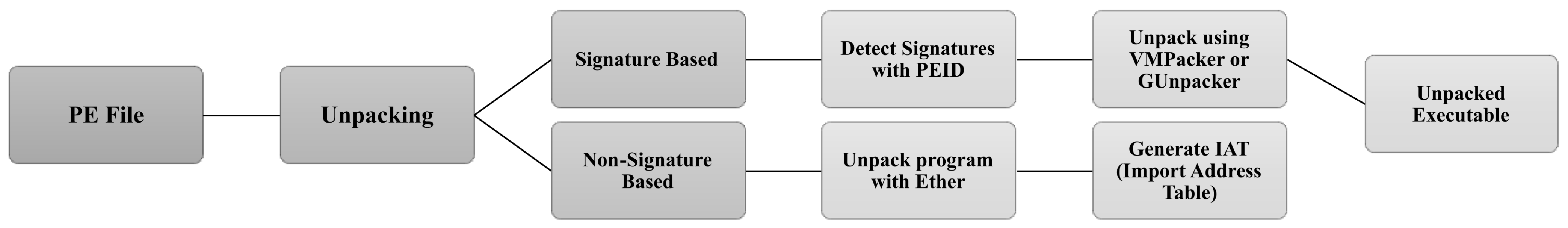
- Disk Image Creation: We created a disk image, this disk image works as a separate hard disk;
- Windows XP Installation: Once the disk image was created, we installed Windows XP on that disk image. We chose Windows XP Service Pack 2 as most of the viruses, written for Windows environments only. Another reason to choose Windows XP Service Pack 2 is that the ether patched version of Xen has been tested with XP SP2 as guest OS and Debian Lenny as host OS;
- Running Ether Patched Xen: Once we have installed the Operating System on Ether patched XEN, we run the machine using the vncviewer [41];
- Unpacking using Ether Patched Xen: To analyze the malware dynamically, the malware is executed on the DomU machine (XP SP2) and its footprints are recorded on the Dom0 system (Debian Lenny).
3.1. Software Armoring
3.2. Feature Extraction
- API Call tracing using Veratrace. Veratrace is an Intel PIN-based API call tracing program for Windows. This program can trace API calls of only de-armored programs obtained from Ether. The output of Veratrace is parsed, and each executable is represented in the form of a vector. The collection of vectors of all applications is represented in the form of a two-dimensional matrix referred to us as the Frequency Vector Table (FVT) of API traces;
- Mnemonics and instruction opcode are extracted using ObjDump [44]. A custom-developed parser transforms the sample to FVT of mnemonics and instruction opcode.
3.3. API Calls Tracing
3.4. Mnemonic, Instruction Opcode, and 4-Gram Mnemonic Trace
3.5. Feature Selection
- Dimension reduction to haul down the computational cost;
- Reduction of noise to boost the classification accuracy;
- Introduce more interpretable features that can help identify and monitor the unknown sample.
3.5.1. Minimum Redundancy Maximum Relevance
- Efficiency: If a feature set of 50 samples contains many mutually highly correlated features, the representative features are very few, say 30, which means that 20 features are redundant, increasing the computational cost;
- Broadness: According to their discriminative powers, we select some attributes, but such feature space is not maximally representative of the original space covered by the entire data set. The feature set may represent one or several dominant characteristics of an unknown sample, but it could also be a narrow region of relevant space. Thus the generalization ability could be limited.
- Relevance value of an attribute x, is computed using Equation (2):where h is the target variable or class, is the mutual information between class and feature x.
- Redundancy value, of feature x is obtained using Equation (3):where N is the total number of attributes, is the mutual information of features and x respectively.
- Mutual Information Difference (MID): Is defined as the difference between the relevance value () and the redundancy value (). To optimize the minimum redundancy and maximum relevance criteria, the difference between the relevance and redundancy value (see Equation (4)) was computed.Hence, the feature with maximum value indicates the mRMR feature;
- Mutual Information Quotient (MIQ): Is obtained by dividing the relevance value with the redundancy value, thus optimizing the mRMR criteria (refer to Equation (5)):
3.5.2. Analysis of Variance
- One way ANOVA: Requires one feature with at least two levels such that the levels are independent;
- Repeated Measures ANOVA: It commands one feature with at least two levels such that the levels are dependent;
- Factorial ANOVA: This approach demands two or more features, each of which with at least two levels either dependent, independent, or mixed.
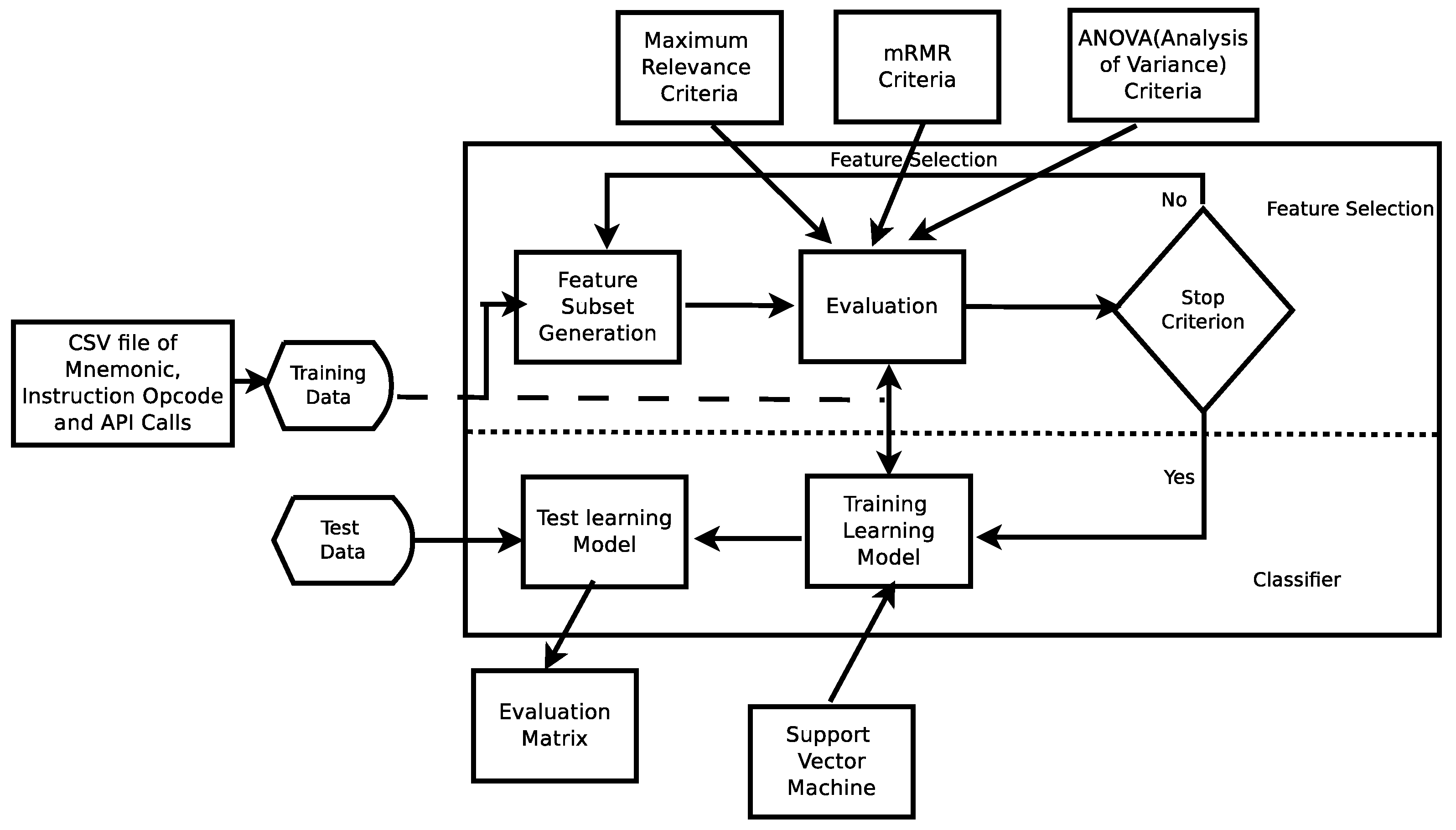
3.6. Classification
- In the first step, we built a classifier describing a predetermined set of classes or concepts, also known as the learning step (or training phase). In this stage, a classification algorithm builds the classifier by analyzing or learning from a training set and their associated class labels. A tuple or feature, X, is represented by an n-dimensional attribute vector, , where, n depicts measurements made on the tuple from n database attributes, respectively, , ,…, . Each tuple, X, is assumed to belong to a predefined class determined by the class label. The labels corresponding to the class attribute is discrete valued and unordered. The individual tuples making up the training set are referred to as training tuples and are randomly selected from the dataset. The class label of each training tuple is known to the classifier already, thus this approach is known as supervised learning;
- In the second step, we use the classification model and predict the test data. This reserved set of samples is never used in the training phase. Eventually, the performance of the model on a given test set is estimated, generally evaluated as the percentage of test set tuples that are correctly classified by the classifier.
4. Experimental Evaluation and Results
4.1. Evaluation Metrics
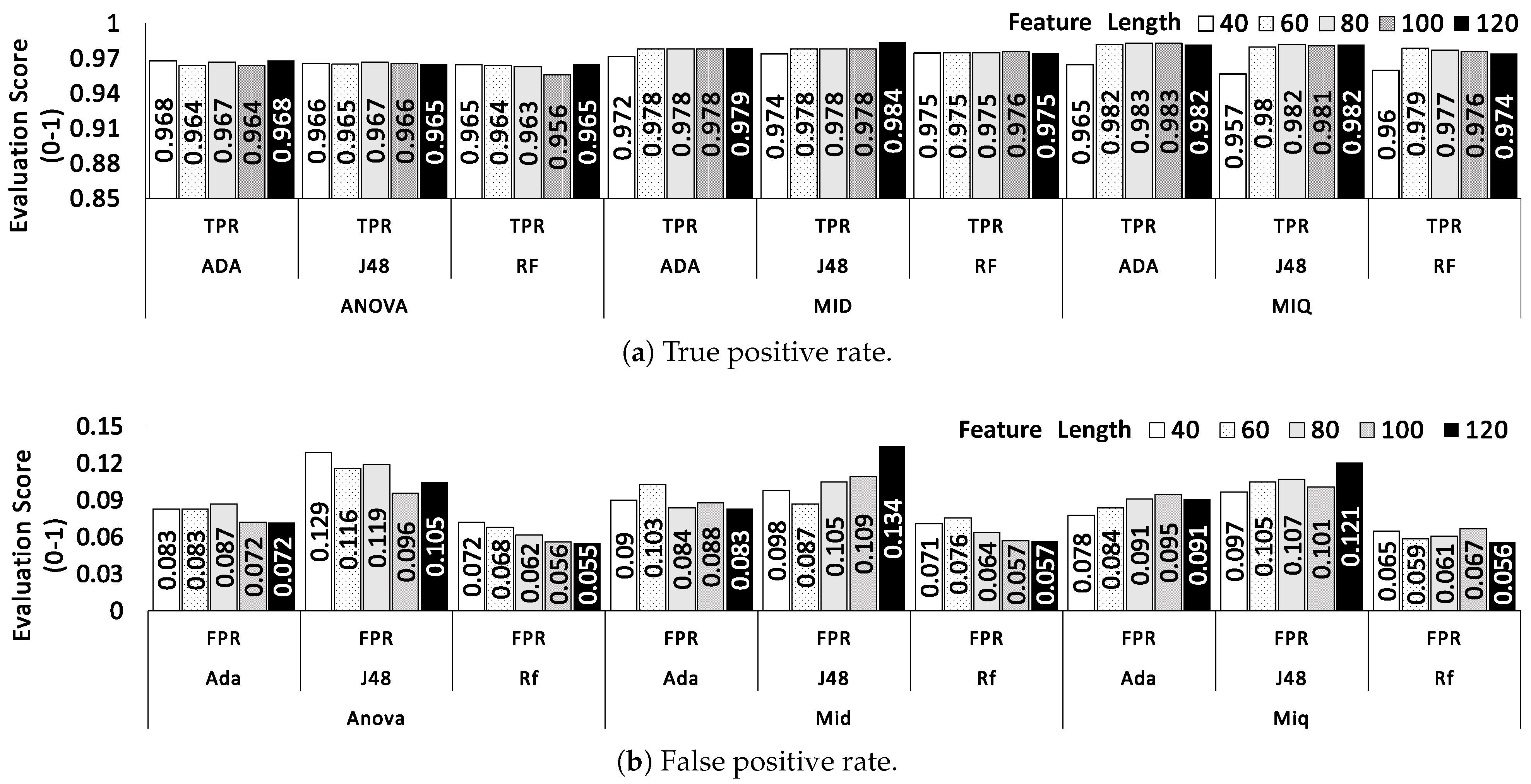
- True Positive Rate () or Recall (R) = ;
- Precision (P) =
- F-measure =
- Accuracy (A) =
4.2. Experiments Results
- Dataset-1 (VX-Dataset): A total of 2000 Portable Executables were collected which consists of 1000 malware samples gathered from sources VxHeaven (650) [35], User Agency (250), and Offensive Computing (100), and benign samples were collected from Windows XP System32 Folder (450), Windows7 System32 Folder (100), MikTex/Matlab Library (400), and Games (50);
- Dataset-2 (Virusshare-Dataset): A total of 622 executables were downloaded from virusshare [36], these belong to malware families like Mediyes, Locker. Intallcore, CryptoRansom, Citadel Zeus, and APT1_293. In addition, we collected 118 benign files from the freshly installed Windows operating system. These samples were used to evaluate the classifier performance on multi-label classification;
- Dataset-3 (Android-Dataset): A total 4000 applications were considered, out of which 2000 malicious samples were randomly chosen from the Derbin project [37], and 2000 legitimate applications were downloaded from the Google Playstore. Each benign application was submitted to the VirusTotal service to validate its genuinity;
- Dataset-4 (Synthetic Samples): VX Heavens reports nearly 152 synthetic kits and a few metamorphic engines to generate functionally equivalent malware code. Phalcon/Skin Mass-Produced Code generator (PS-MPCs), Second Generation virus-generator (G2), Mass Code Generator (MPCGEN), Next Generation Virus Creation Kit (NGCVK), and Virus Creation Lab for Win32 (VCL32) are widely used to generate synthetic malware. A total of 320 viruses were generated with virus constructors and used as training samples. A separate test set is considered which includes 95 viruses (20 viruses from each generator and 15 real metamorphic) and 20 benign samples.
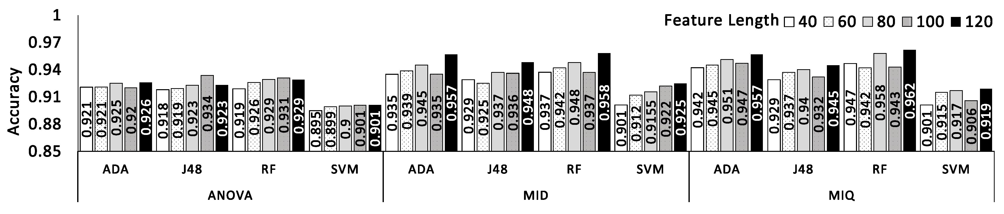
4.3. Investigation of Relevant Feature Type-Dataset-1
4.4. Evaluation on Virusshare Samples Dataset-2
4.5. Evaluation on Android Applications Dataset-3
4.6. Evaluation on Synthetic Samples Dataset-4
5. Conclusions and Future Work
Author Contributions
Funding
Acknowledgments
Conflicts of Interest
Abbreviations
| List of Abbreviations | |
| 1D-CNN | One-Dimensional Convolutional Neural Network |
| ANOVA | Analysis of Variance |
| API | Application Programming Interface |
| AV | AntiVirus |
| CART | Classification and Regression Tree |
| CNN | Convolutional Neural Network |
| CNN-LSTM | CNN Long Short-Term Memory Network |
| DNN | Deep Neural Network |
| FN | False Negative |
| FP | False Positive |
| FPR | False Positive Rate |
| FVT | Frequency Vector Table |
| G2 | Second Generation Virus Generator |
| HMMs | Hidden Markov Models |
| k-NN | K-Nearest Neighbors |
| MID | Mutual Information Difference |
| MIQ | Mutual Information Quotient |
| MPCGEN | Mass Produced Code Generation Kit |
| mRMR | Minimum Redundancy and Maximum Relevance |
| NGVCK | Next Generation Virus Construction Kit |
| OS | Operating System |
| PE | Portable Executables |
| PSMPC | Phalcon/Skin Mass–Produced Code generator |
| QEMU | Quick EMUlator |
| ReLU | Rectified Linear Activation Function |
| RF | Random Forest |
| SMS | Short Message Service |
| SVM | Support Vector Machine |
| syscall | System Call |
| TF-IDF | Term Frequency Inverse Document Frequency |
| TPR | True Positive Rate |
| R | Recall |
| RDTSC | Read Time Stamp Counter |
| P | Precision |
| TP | True Positive |
| TN | True Negative |
| FP | False Positive |
| FN | False Negative |
| VCL32 | Virus Creation Lab for Win32 |
| XGBoost | eXtreme Gradient Boosting |
| List of Mathematical Symbols | |
| Summation notation | |
| log | Logarithm |
| Features or Attributes | |
| Probability distribution of x | |
| Mutual information between feature x and y | |
| Joint probabilistic distribution of feature x and y | |
| Marginal probabilities of x and y | |
| i | Level or state of feature x |
| j | Level or state of feature y |
| S | Set obtained from cross product of set of states of x and y |
| Relevance value of an attribute x | |
| h | Target variable or class |
| Mutual information between class h and feature x. | |
| Redundancy value of feature x | |
| N | Total number of attributes |
| Mutual information of features and x respectively | |
| Difference between the relevance value and the redundancy value | |
| Obtained by dividing the relevance value with the redundancy Value | |
| Sum of squares of feature p belonging to group B | |
| Sum of squares of feature p belonging to group W | |
| Total sum of squares of feature p | |
| k | Number of classes (malware/benign) |
| l | Number of states of feature p |
| Mean of frequencies of feature p | |
| Feature at class I and state j | |
| Mean of frequencies of feature p in ith discretization state | |
| Degree of freedom of feature p within the group W | |
| Number of observations of feature p | |
| Number of samples of feature p | |
| Degree of freedom of feature p between the group B | |
| F-score | |
| X | A tuple or feature represented by an n-dimensional attribute vector |
References
- Saraiva, D.A.; Leithardt, V.R.Q.; de Paula, D.; Sales Mendes, A.; González, G.V.; Crocker, P. Prisec: Comparison of symmetric key algorithms for iot devices. Sensors 2019, 19, 4312. [Google Scholar] [CrossRef] [PubMed] [Green Version]
- Bulazel, A.; Yener, B. A survey on automated dynamic malware analysis evasion and counter-evasion: Pc, mobile, and web. In Proceedings of the 1st Reversing and Offensive-Oriented Trends Symposium, Vienna, Austria, 16–17 November 2017; pp. 1–21. [Google Scholar] [CrossRef]
- Mandiant. Available online: https://www.fireeye.com/mandiant.html (accessed on 6 July 2021).
- Dinaburg, A.; Royal, P.; Sharif, M.; Lee, W. Ether: Malware analysis via hardware virtualization extensions. In Proceedings of the 15th ACM Conference on Computer and Communications Security, Alexandria, VA, USA, 27–31 October 2008; ACM: New York, NY, USA, 2008; pp. 51–62. [Google Scholar] [CrossRef]
- Alaeiyan, M.; Parsa, S.; Conti, M. Analysis and classification of context-based malware behavior. Comput. Commun. 2019, 136, 76–90. [Google Scholar] [CrossRef]
- Intel. Available online: http://www.intel.com/ (accessed on 6 July 2021).
- Virus Total. Available online: https://www.virustotal.com/en/statistics/ (accessed on 6 July 2021).
- Christodorescu, M.; Jha, S.; Kruegel, C. Mining specifications of malicious behavior. In Proceedings of the the 6th Joint Meeting of the European Software Engineering Conference and the ACM SIGSOFT Symposium on the Foundations of Software Engineering, Dubrovnik, Croatia, 3–7 September 2007; ACM: New York, NY, USA, 2007; pp. 5–14. [Google Scholar] [CrossRef]
- Alzaylaee, M.K.; Yerima, S.Y.; Sezer, S. DL-Droid: Deep learning based android malware detection using real devices. Comput. Secur. 2020, 89, 101663. [Google Scholar] [CrossRef]
- Canfora, G.; Medvet, E.; Mercaldo, F.; Visaggio, C.A. Detecting Android malware using sequences of system calls. In Proceedings of the 3rd International Workshop on Software Development Lifecycle for Mobile, Bergamo, Italy, 31 August 2015; pp. 13–20. [Google Scholar] [CrossRef]
- Wang, W.; Li, Y.; Wang, X.; Liu, J.; Zhang, X. Detecting Android malicious apps and categorizing benign apps with ensemble of classifiers. Future Gener. Comput. Syst. 2018, 78, 987–994. [Google Scholar] [CrossRef] [Green Version]
- Nataraj, L.; Karthikeyan, S.; Jacob, G.; Manjunath, B. Malware images: Visualization and automatic classification. In Proceedings of the 8th International Symposium on Visualization for Cyber Security, Pittsburgh, PA, USA, 20 July 2011; pp. 1–7. [Google Scholar] [CrossRef]
- Ni, S.; Qian, Q.; Zhang, R. Malware identification using visualization images and deep learning. Comput. Secur. 2018, 77, 871–885. [Google Scholar] [CrossRef]
- Yuan, Z.; Lu, Y.; Xue, Y. Droiddetector: Android malware characterization and detection using deep learning. Tsinghua Sci. Technol. 2016, 21, 114–123. [Google Scholar] [CrossRef]
- McLaughlin, N.; Martinez del Rincon, J.; Kang, B.; Yerima, S.; Miller, P.; Sezer, S.; Safaei, Y.; Trickel, E.; Zhao, Z.; Doupé, A.; et al. Deep android malware detection. In Proceedings of the Seventh ACM on Conference on Data and Application Security and Privacy, Scottsdale, AZ, USA, 22–24 March 2017; pp. 301–308. [Google Scholar] [CrossRef] [Green Version]
- Karbab, E.B.; Debbabi, M.; Derhab, A.; Mouheb, D. Android malware detection using deep learning on API method sequences. arXiv 2017, arXiv:1712.08996. [Google Scholar]
- Iadarola, G.; Martinelli, F.; Mercaldo, F.; Santone, A. Towards an Interpretable Deep Learning Model for Mobile Malware Detection and Family Identification. Comput. Secur. 2021, 105, 102198. [Google Scholar] [CrossRef]
- Zhang, B.; Yin, J.; Hao, J. Using Fuzzy Pattern Recognition to Detect Unknown Malicious Executables Code. In Fuzzy Systems and Knowledge Discovery; Lecture Notes in Computer Science; Springer: Berlin/Heidelberg, Germany, 2005; Volume 3613, pp. 629–634. [Google Scholar] [CrossRef]
- Sun, H.M.; Lin, Y.H.; Wu, M.F. API Monitoring System for Defeating Worms and Exploits in MS-Windows System. In Information Security and Privacy; Springer: Berlin/Heidelberg, Germany, 2006; Volume 4058, pp. 159–170. [Google Scholar] [CrossRef]
- Bergeron, J.; Debbabi, M.; Erhioui, M.M.; Ktari, B. Static Analysis of Binary Code to Isolate Malicious Behaviors. In Proceedings of the 8th Workshop on Enabling Technologies on Infrastructure for Collaborative Enterprises, Palo Alto, CA, USA, 16–18 June 1999; IEEE Computer Society: Washington, DC, USA, 1999; pp. 184–189. [Google Scholar] [CrossRef]
- Zhang, Q.; Reeves, D.S. MetaAware: Identifying Metamorphic Malware. In Proceedings of the Twenty-Third Annual Computer Security Applications Conference (ACSAC 2007), Miami Beach, FL, USA, 10–14 December 2007; pp. 411–420. [Google Scholar] [CrossRef] [Green Version]
- Sathyanarayan, V.S.; Kohli, P.; Bruhadeshwar, B. Signature Generation and Detection of Malware Families. In Proceedings of the 13th Australasian Conference on Information Security and Privacy, Wollongong, Australia, 7–9 July 2008; Springer: Berlin/Heidelberg, Germany, 2008; pp. 336–349. [Google Scholar] [CrossRef]
- Rabek, J.C.; Khazan, R.I.; Lewandowski, S.M.; Cunningham, R.K. Detection of injected, dynamically generated, and obfuscated malicious code. In Proceedings of the 2003 ACM Workshop on Rapid Malcode, Washington, DC, USA, 27 October 2003; ACM: New York, NY, USA, 2003; pp. 76–82. [Google Scholar] [CrossRef]
- Damodaran, A.; Di Troia, F.; Visaggio, C.A.; Austin, T.H.; Stamp, M. A comparison of static, dynamic, and hybrid analysis for malware detection. J. Comput. Virol. Hacking Tech. 2017, 13, 1–12. [Google Scholar] [CrossRef]
- Wong, W.; Stamp, M. Hunting for metamorphic engines. J. Comput. Virol. 2006, 2, 211–229. [Google Scholar] [CrossRef]
- Nair, V.P.; Jain, H.; Golecha, Y.K.; Gaur, M.S.; Laxmi, V. MEDUSA: MEtamorphic malware dynamic analysis using signature from API. In Proceedings of the 3rd International Conference on Security of Information and Networks, Taganrog, Russia, 7–11 September 2010; ACM: New York, NY, USA, 2010; pp. 263–269. [Google Scholar] [CrossRef]
- Suarez-Tangil, G.; Stringhini, G. Eight years of rider measurement in the android malware ecosystem: Evolution and lessons learned. arXiv 2018, arXiv:1801.08115. [Google Scholar]
- Zhou, Y.; Jiang, X. Dissecting Android Malware: Characterization and Evolution. In Proceedings of the 33rd IEEE Symposium on Security and Privacy (Oakland 2012), San Francisco, CA, USA, 21–23 May 2012. [Google Scholar] [CrossRef] [Green Version]
- Arp, D.; Spreitzenbarth, M.; Huebner, M.; Gascon, H.; Rieck, K. Drebin: Efficient and Explainable Detection of Android Malware in Your Pocket. In Proceedings of the 21st Annual Network and Distributed System Security Symposium (NDSS), San Diego, CA, USA, 23–26 February 2014. [Google Scholar]
- Yan, L.K.; Yin, H. DroidScope: Seamlessly Reconstructing the OS and Dalvik Semantic Views for Dynamic Android Malware Analysis. In Proceedings of the 21st USENIX Conference on Security Symposium, Bellevue, WA, USA, 8–10 August 2012; USENIX Association: Berkeley, CA, USA, 2012; p. 29, ISBN 978-931971-95-9. [Google Scholar]
- Canfora, G.; Mercaldo, F.; Visaggio, C.A. A classifier of Malicious Android Applications. In Proceedings of the 2nd International Workshop on Security of Mobile Applications, in Conjunction with the International Conference on Availability, Reliability and Security, Regensburg, Germany, 2–6 September 2013. [Google Scholar] [CrossRef]
- Su, D.; Liu, J.; Wang, W.; Wang, X.; Du, X.; Guizani, M. Discovering communities of malapps on Android-based mobile cyber-physical systems. Ad Hoc Netw. 2018, 80, 104–115. [Google Scholar] [CrossRef] [Green Version]
- Liu, X.; Liu, J.; Zhu, S.; Wang, W.; Zhang, X. Privacy risk analysis and mitigation of analytics libraries in the android ecosystem. IEEE Trans. Mob. Comput. 2019, 19, 1184–1199. [Google Scholar] [CrossRef] [Green Version]
- Casolare, R.; Martinelli, F.; Mercaldo, F.; Santone, A. Detecting Colluding Inter-App Communication in Mobile Environment. Appl. Sci. 2020, 10, 8351. [Google Scholar] [CrossRef]
- VX Heavens. Available online: https://vx-underground.org/archive/VxHeaven/index.html (accessed on 6 July 2021).
- Virusshare. Available online: https://virusshare.com/ (accessed on 6 July 2021).
- Drebin. Available online: https://www.sec.cs.tu-bs.de/~danarp/drebin/download.html (accessed on 6 July 2021).
- Alkhateeb, E.; Stamp, M. A Dynamic Heuristic Method for Detecting Packed Malware Using Naive Bayes. In Proceedings of the 2019 International Conference on Electrical and Computing Technologies and Applications (ICECTA), Ras Al Khaimah, United Arab Emirates, 19–21 November 2019; pp. 1–6. [Google Scholar] [CrossRef]
- Xen Project. Available online: http://www.xen.org (accessed on 6 July 2021).
- Windows API Library. Available online: https://docs.microsoft.com/en-us/windows/win32/apiindex/windows-api-list (accessed on 6 July 2021).
- Vnc Viewer. Available online: https://www.realvnc.com/en/connect/ (accessed on 6 July 2021).
- You, I.; Yim, K. Malware obfuscation techniques: A brief survey. In Proceedings of the 2010 International Conference on Broadband, Wireless Computing, Communication and Applications, Fukuoka, Japan, 4–6 November 2010; pp. 297–300. [Google Scholar] [CrossRef]
- Borello, J.M.; Mé, L. Code obfuscation techniques for metamorphic viruses. J. Comput. Virol. 2008, 4, 211–220. [Google Scholar] [CrossRef]
- ObjDump. Available online: https://web.mit.edu/gnu/doc/html/binutils_5.html (accessed on 6 July 2021).
- Witten, I.; Frank, E. Practical Machine Learning Tools and Techniques with Java Implementation; Morgan Kaufmann: Burlington, MA, USA, 1999; ISBN 1-55860-552-5. [Google Scholar]
- Factorial Anova. Available online: http://en.wikipedia.org/wiki/Analysis_of_variance (accessed on 6 July 2021).
- Ding, C.; Peng, H. Minimum Redundancy Feature Selection from Microarray Gene Expression Data. In Proceedings of the IEEE Computer Society Conference on Bioinformatics, Stanford, CA, USA, 11–14 August 2003; p. 523. [Google Scholar] [CrossRef]
- Cortes, C.; Vapnik, V. Support-vector networks. Mach. Learn. 1995, 20, 273–297. [Google Scholar] [CrossRef]
- Rish, I. An empirical study of the naive Bayes classifier. In Proceedings of the IJCAI 2001 Workshop on Empirical Methods in Artificial Intelligence, Seattle, WA, USA, 4 August 2001; Volume 3, pp. 41–46. [Google Scholar]
- Quinlan, J.R. C4.5: Programs for Machine Learning; Elsevier: Amsterdam, The Netherlands, 2014; ISBN 1-55860-238-0. [Google Scholar]
- Breiman, L. Random forests. Mach. Learn. 2001, 45, 5–32. [Google Scholar] [CrossRef] [Green Version]
- Chen, T.; Guestrin, C. Xgboost: A scalable tree boosting system. In Proceedings of the 22nd Acm Sigkdd International Conference on Knowledge Discovery and Data Mining, San Francisco, CA, USA, 13–17 August 2016; pp. 785–794. [Google Scholar] [CrossRef] [Green Version]
- Narudin, F.A.; Feizollah, A.; Anuar, N.B.; Gani, A. Evaluation of machine learning classifiers for mobile malware detection. Soft Comput. 2016, 20, 343–357. [Google Scholar] [CrossRef]
- Singh, J.; Singh, J. A survey on machine learning-based malware detection in executable files. J. Syst. Archit. 2021, 112, 101861. [Google Scholar] [CrossRef]
- Mahdavifar, S.; Ghorbani, A.A. Application of deep learning to cybersecurity: A survey. Neurocomputing 2019, 347, 149–176. [Google Scholar] [CrossRef]
- Raff, E.; Zak, R.; Cox, R.; Sylvester, J.; Yacci, P.; Ward, R.; Tracy, A.; McLean, M.; Nicholas, C. An investigation of byte n-gram features for malware classification. J. Comput. Virol. Hacking Tech. 2018, 14, 1–20. [Google Scholar] [CrossRef]
- Lin, D.; Stamp, M. Hunting for undetectable metamorphic viruses. J. Comput. Virol. 2011, 7, 201–214. [Google Scholar] [CrossRef] [Green Version]


| Machine Learning-Based Techniques | ||
|---|---|---|
| Author | Approach | Drawback |
| M. Christodorescu et al. [8] | Mine malicious behavior present in a known malware. | The impact of test program choices on the quality of mined malware behavior was not clear. |
| M. K. Alzaylaee et al. [9] | Deep learning system that detects malicious Android applications through dynamic analysis using stateful input generation. | Investigation on recent intrusion detection systems were not available. |
| G. Canfora et al. [10] | Android malware detection method based on sequences of system calls. | Assumption that malicious behaviors are implemented by specific system calls sequences. |
| W. Wang et al. [11] | Framework to effectively and efficiently detect malicious apps and benign apps. | Require datasets of features extracted from malware and harmless samples in order to train their models. |
| L. Nataraj et al. [12] | Effective method for visualizing and classifying malware using image processing techniques. | Path to a broader spectrum of novel ways to analyze malware was not fully explored. |
| Deep Learning-Based Techniques | ||
| Author | Approach | Drawback |
| S. Ni et al. [13] | Classification algorithm that uses static features called Malware Classification using SimHash and CNN. | Time required for malware detection and classification was comparatively more. |
| Z. Yuan et al. [14] | An online deep learning-based Android malware detection engine (DroidDetector). | The semantic-based features of Android malware were not considered. |
| N. McLaughlin et al. [15] | A novel Android malware detection system that uses a deep convolutional neural network. | The same network architecture cannot be applied to malware analysis on different platforms. |
| E. B. Karbab et al. [16] | Android malware detection using deep learning on API method sequences. | Less affected by the obfuscation techniques because they only consider the API method calls. |
| G. Iadarola et al. [17] | Deep learning model for mobile malware detection and family identification. | Model needs to be trained with large sets of labeled data. |
| Other Techniques | ||
| Author | Approach | Drawback |
| B. Zhang et al. [18] | Detect unknown malicious executables code using fuzzy pattern recognition. | Fuzzy pattern recognition algorithm suffers from a low detection and accuracy rate. |
| H. M. Sun et al. [19] | Detecting worms and other malware by using sequences of WinAPI calls. | Approach is limited to the detection of worms and exploits the use of hard-coded addresses of API calls. |
| J. Bergeron et al. [20] | Proposed a slicing algorithm for disassembling binary executables. | Graphs created are huge in size, thus the model is not computationally feasible. |
| Q. Zhang et al. [21] | Approach for recognizing metamorphic malware by using fully automated static analysis of executables. | Absence of analysis of the parameters passed to library or system functions. |
| V. S. Sathyanarayan et al. [22] | Static extraction to extract API calls from known malware in order to construct a signature for an entire class. | Detection of malware families does not work for packed malware. |
| J. C. Rabek et al. [23] | Host-based technique for detecting several general classes of malicious code in software executables. | Not applicable for detecting all malicious code in executable. |
| A. Damodaran et al. [24] | Comparison of malware detection techniques based on static, dynamic, and hybdrid analysis. | Disadvantage is that it is thwarted easily by obfuscation techniques. |
| W. Wong et al. [25] | Method for detecting metamorphic viruses using Hidden Markov models. | Model can be defeated by inserting a sufficient amount of code from benign files into each virus |
| V. P. Nair et al. [26] | Tracing malware API calls via dynamic monitoring within an emulator to extract critical APIs. | Applicability of the method to detection of new malware families are limited. |
| G. Suarez-Tangi et al. [27] | Differential analysis to isolate software components that are irrelevant to study the behavior of malicious riders. | Study is vulnerable to update attacks since the payload is stored in a remote host. |
| Y. Zhou et al. [28] | Android platform with the aim to systematize or characterize existing Android malware. | Detection of Android malware that shows the rapid development and increased sophistication, posing significant challenges to this system. |
| L. K. Yan et al. [30] | DroidScope, an Android analysis platform that continues the tradition of virtualization-based malware analysis. | Overall performance of the model is less, compared to others. |
| G. Canfora et al. [31] | Method for detecting malware based on the occurrences of a specific subset of system calls, a weighted sum of a subset of permissions. | Precise patterns and sequences of system calls that could be recurrent in malicious code fragments were ignored. |
| D. Su et al. [32] | Automated community detection method for Android malware apps by building a relation graph based on their static features. | This method for malware app family classification is not as precise as supervised learning approaches. |
| X. Liu et al. [33] | Collect and analyze users action (API) on an Android platform to detect privacy leakage. | Fail when tracking APIs used by other apps that are not listed in the configure file. |
| R. Casolare et al. [34] | Static approach, based on formal methods, which exploit the model checking technique. | Limitations of method is that the generation of the first heuristic is not automatic. |
| Model | Precision (%) | Recall (%) | F1-Score (%) | Accuracy (%) |
|---|---|---|---|---|
| DNN | 99.1 | 99.1 | 99.1 | 99.1 |
| 1D-CNN | 97.9 | 97.9 | 97.9 | 97.9 |
| CNN-LSTM | 69.4 | 79.6 | 73.4 | 79.6 |
| XGBOOST | 97.8 | 97.8 | 97.5 | 97.8 |
| Random Forest | 97.3 | 97.25 | 96.89 | 97.35 |
| AdaBoostM1 | 96.8 | 97.8 | 96.4 | 97.0 |
| SVM | 89.28 | 88.24 | 88.72 | 86.8 |
| J48 | 87.54 | 88.08 | 87.6 | 86.53 |
| Model | Topology |
|---|---|
| DNN | Dense1_units = 100; Dropout = 0.2; Activation = relu; Dense2_units = 50; Dropout = 0.2; Activation = relu; dense_final_units: 6; Activation = softmax; Optimizer: Adam; Learning rate: 0.001; batch size = 128, epoch = 40 |
| 1D-CNN | Conv1D: (num_filters = 15, filter_size: 2); Activation = relu; Maxpooling1D; Conv1D: (num_filters = 15, filter_size = 2); Activation = relu; Maxpooling1D; Flatten; Dense units = 100; Activation: relu; dropout = 0.05; dense_ final_units = 6; Activation = Softmax; optimizer = Adam, epoch = 15 |
| SVM | kernel = rbf; gamma = 1; max_iter = 500; decision_function_shape = ovo |
| XGBOOST | XGBClassifier() |
| CNN-LSTM | Conv1D: ( num_filters = 15, filter_size = 2); Activation: relu; maxpooling1D; LSTM_units = 100; Dense_units = 100; Activation = relu; Dropout = 0.05; Dense_units = 50; Activation = relu; Dropout = 0.05; Dense_final_units = 6; Activation = softmax; Optimizer = adam |
| Classifier | Accuracy | F1-Measure | TPR | AUC |
|---|---|---|---|---|
| Random Forest | 97.80% | 97.8% | 97.7% | 0.998 |
| AdaBoostM1 | 97.37% | 96.4% | 96.8% | 0.97 |
| J48 | 95.12% | 95.1% | 96.0% | 0.965 |
| SVM | 95.02% | 95.3% | 95.1% | 0.963 |
| XGBoost | 99.82% | 99.82% | 99.71% | 0.998 |
| Dropout | Accuracy (%) | F1-Score (%) | Precision (%) | Recall (%) |
|---|---|---|---|---|
| 0.1 | 98.48 | 98.48 | 98.48 | 98.48 |
| 0.2 | 97.92 | 97.92 | 97.97 | 97.87 |
| 0.3 | 98.38 | 98.38 | 98.48 | 98.28 |
| 0.4 | 98.13 | 98.14 | 97.41 | 98.89 |
| 0.5 | 98.03 | 98.04 | 97.50 | 98.58 |
| 0.6 | 97.97 | 97.96 | 98.57 | 97.37 |
| Classifier | Accuracy (%) | F-Measure (%) | Precision (%) | Recall (%) |
|---|---|---|---|---|
| J48 | 99.5 | 99.4 | 99.5 | 99.3 |
| AdaboostMI(J48) | 99.5 | 99.4 | 99.5 | 99.3 |
| Random Forest | 99.7 | 99.6 | 99.5 | 99.7 |
| Constructors | Number of Families | Number of Variants |
|---|---|---|
| NGVCK | 5 | 21 |
| G2 | 5 | 21 |
| PSMPC | 5 | 21 |
| MPCGEN | 5 | 21 |
| Real Malware Samples | 11 | 5–77 |
| Sample 1 | Sample 2 |
|---|---|
| push | push |
| retn | retn |
| # - | mov |
| # - | sub |
| and | and |
| lea | lea |
| mov | mov |
| mov | mov |
| # - | popa |
| # - | sub |
| jmp | jmp |
| * inc | mov |
| * shr | and |
| * ror | mov |
| * cmp | dec |
| NGVCK | G2 | PSMPC | MPCGEN |
|---|---|---|---|
| add mov | int call | jnz loop | mov pop |
| push mov | mov pop | - | cmp mov |
| mov pop | lea mov | - | int mov |
| call mov | xor cwd | - | mov lea |
| mov sub | mov movsb | - | jmp int |
| push add | rep movsb | - | call add |
| mov xor | xor mov | - | add movsw |
| and mov | cwd mov | - | lea jmp |
| mov jz | int inc | - | movsw mov |
| mov cmp | movsb movsw | - | push pop |
Publisher’s Note: MDPI stays neutral with regard to jurisdictional claims in published maps and institutional affiliations. |
© 2021 by the authors. Licensee MDPI, Basel, Switzerland. This article is an open access article distributed under the terms and conditions of the Creative Commons Attribution (CC BY) license (https://creativecommons.org/licenses/by/4.0/).
Share and Cite
Ashik, M.; Jyothish, A.; Anandaram, S.; Vinod, P.; Mercaldo, F.; Martinelli, F.; Santone, A. Detection of Malicious Software by Analyzing Distinct Artifacts Using Machine Learning and Deep Learning Algorithms. Electronics 2021, 10, 1694. https://doi.org/10.3390/electronics10141694
Ashik M, Jyothish A, Anandaram S, Vinod P, Mercaldo F, Martinelli F, Santone A. Detection of Malicious Software by Analyzing Distinct Artifacts Using Machine Learning and Deep Learning Algorithms. Electronics. 2021; 10(14):1694. https://doi.org/10.3390/electronics10141694
Chicago/Turabian StyleAshik, Mathew, A. Jyothish, S. Anandaram, P. Vinod, Francesco Mercaldo, Fabio Martinelli, and Antonella Santone. 2021. "Detection of Malicious Software by Analyzing Distinct Artifacts Using Machine Learning and Deep Learning Algorithms" Electronics 10, no. 14: 1694. https://doi.org/10.3390/electronics10141694
APA StyleAshik, M., Jyothish, A., Anandaram, S., Vinod, P., Mercaldo, F., Martinelli, F., & Santone, A. (2021). Detection of Malicious Software by Analyzing Distinct Artifacts Using Machine Learning and Deep Learning Algorithms. Electronics, 10(14), 1694. https://doi.org/10.3390/electronics10141694