Approaching Optimal Nonlinear Dimensionality Reduction by a Spiking Neural Network

Abstract

This work deals with the presentation of a spiking neural network as a means for efficiently solving the reduction of dimensionality of data in a nonlinear manner. The underneath neural model, which can be integrated as neuromorphic hardware, becomes suitable for intelligent processing in edge computing within Internet of Things systems. In this sense, to achieve a meaningful performance with a low complexity one-layer spiking neural network, the training phase uses the metaheuristic Artificial Bee Colony algorithm with an objective function from the principals in the machine learning science, namely, the modified Stochastic Neighbor Embedding algorithm. To demonstrate this fact, complex benchmark data were used and the results were compared with those generated by a reference network with continuous-sigmoid neurons. The goal of this work is to demonstrate via numerical experiments another method for training spiking neural networks, where the used optimizer comes from metaheuristics. Therefore, the key issue is defining the objective function, which can relate optimally the information at both sides of the spiking neural network. Certainly, machine learning techniques have advanced in defining efficient loss functions that can become suitable objective function candidates in the metaheuristic training phase. The practicality of these ideas is shown in this article. We use MSE values for evaluating the relative quality of the results and also co-ranking matrices.

1. Introduction

Present and following information systems demand reviewing intelligent processes for their efficiency. A sample of this dynamic issue is drawn from [1], where three “influence-domain” categories, i.e., information processing, information transmission, and learning strategy, lead the analysis of existing deep learning architectures. On the other hand, from the context of the neuromorphic system, the computational spiking hardware is recognized as both energy-efficient and reliable, where mostly the spike-timing-dependent plasticity rule (STDP rule) is used for setting the weighting values of the synaptic connections, i.e., the learning rule [2]. In these architectures, layers of spiking neurons are aimed to resemble the temporal encoding of the information communication as it occurs in biological neural systems. The STDP rule represents the central mechanism for modifying the conductance value in biological synapses. Multilayer, recurrent, and hybrid spiking architectures along with their training algorithms are reviewed in [3] and show that the classic back-propagation method can be adapted for the spiking models, finding that it is not quite efficient for dealing with spatiotemporal information flows. The same work concludes that proposing new learning methods is still an open issue, observing as a goal their performance improvement. Reports on neuromorphic hardware implementations include similar arguments [4]. Taking the learning rule of the spiking neural systems as a pure optimization problem, mature metaheuristic algorithms might contribute to establishing efficient solutions for it. Based on this idea, king neurons to compute efficiently the nonlinear dimensionality reduction of complex data, visualizing their inner classes in 3D spaces. The authors in [5] made a review over two decades on feedforward continuous neural networks. These systems were optimized with metaheuristics and classified into four categories, connection weight, architecture, node, and learning rule. On the other hand, training spiking systems based on metaheuristics could be divided into two branches, firing rate and spike-time delay. The works in [6,7,8] belong to the first category meanwhile those cited in [9,10,11] to the second one. The cuckoo search algorithm in [6], which uses a random walk strategy, achieves the spiking training phase on six complex databases. The authors in [7] reported using the ABC algorithm to train a single spiking neuron, which recognizes classes in 5 datasets and a circular object from an image. Their training strategy was based on the number of correct classification cases in a supervised manner. They concluded that the ABC algorithm improves the quality of the results compared with earlier metaheuristic methods. The work in [8] trains with the ABC algorithm a one-layer spiking neural network to reduce the dimension of complex datasets into 3D spaces in a linear way. In improving the training of spiking systems, similar researchers are found in [9,10] a decade apart. Both use evolutionary algorithms. The research contribution in [9] comes from its parallel version and that in [10] due to its comparison among using three evolutionary versions. The work in [11] deals with an advanced training technique, where a grammatical evolution engine guided outmost the performance. A three-layer spiking network architecture served as a demonstrating vehicle. At last, the work in [12] seems to be a good metaheuristic paradigm that gets an optimal balance between exploration and exploitation, which is reported as reducing overfitting. Although, their authors report low performance in a particular classification problem. In the present article, we argue that the loss function in the t-SNE machine learning method provides its information-representation properties to the spiking neural network during training. It happens because this loss function can act as the objective function in the ABC algorithm. Making a summary, the goal of this article focuses on a three-fold purpose. Firstly, introducing the ABC algorithm as a robust optimizer, because it can discard the appearing local minima in the used objective function, which conversely becomes a burden in front of gradient-based optimization methods. Secondly, taking advantage of the optimal information-representation that the available loss functions have from machine learning methods. Thirdly, combining both the ABC algorithm and a machine learning loss function to solve efficiently a nonlinear dimensionality reduction problem. On the other hand, the technological capabilities associated with the spiking neural network model used in the experiments of this work can lead to hardware realizations. Finally, we review in brief the edge computing advantages that might be associated with IoT systems and list the singular characteristics that our spiking neural network introduces into a neuromorphic system.

2. Main Topics

Current IoT technology can get both intelligence with edge computing and energy efficiency with neuromorphic hardware. These associations are conceived in this work due to the introduction of a metaheuristic process that optimizes a spiking neural network, making possible a type of this hardware. The following seven subsections deal with the topics that indirectly argue in favor of this concept.

2.1. Dimensionality Reduction

One of the topics in machine learning research is related to reducing the dimensionality of complex data, i.e., discovering the classes and the relevant information that represent them. In the linear sense of reducing the dimensionality, the classic Principal Component Analysis (PCA) method computes the eigenvectors and eigenvalues of the covariance matrix of the data set, which denote the new or principal directions on which the classes might be interpreted [13]. The neural architecture for approaching PCA is based on the linear auto-encode [14], whose diagram is depicted in Figure 1. Its training phase can be regarded in two parts, i.e., (1) there are two neuron layers namely, the bottleneck layer and the output layer, whose encoding and decoding weights reach optimal values in the MSE sense, and according to an auto-association task; then, (2) the output layer can be discarded, leaving the bottleneck layer and its encoding weights already able to approach PCA of new data.

This training process can be extended into deeper layers, but considering nonlinear neurons and appropriate loss functions to continue discovering efficiently other relevant features [15]. Based on this background and with the aim at reducing efficiently the dimensionality of input data, we propose using only the Bottleneck layer with nonlinear spiking neurons along with their encoding weights. This minimal spiking network architecture would be trained with the ABC algorithm, becoming the subject of this work and leading to propose a neuromorphic hardware realization. Likewise, we observe that this effort can benefit intelligent IoT systems.

2.2. Internet of Things

The Internet of Things was defined in its origin as a subnetwork to allow instruments, measuring and monitoring devices and mobile communications systems, collect data derived from human being activities for their living support, such as health care, environmental, smart city, commercial and industrial [16]. Technically, the goal in IoT systems was conceived to provide an initial platform from where the information could be sent to specific centers for their analysis, evaluation, and diagnosis; then, after conducting a decision-making process a signal was sent elsewhere through the internet-road for the action of control, security or other.

2.3. Edge Computing

At present, Internet of Things systems are becoming the first link among others on the path between the source and the destination of internet connections and where the edge computing scheme is introduced. This fact brings computing intelligence and security capabilities into the data generation domain. Hence, IoT systems can benefit from deep learning methods, which do efficient information reduction tasks with knowledge discovery [17,18]; this has the impact of optimizing costs and safety of wide-area-networks, clouds and data centers. Likewise, the trend of edge computing with intelligence includes creating frameworks and design standards to define smart IoT architectures. This type of framework is found in [19].

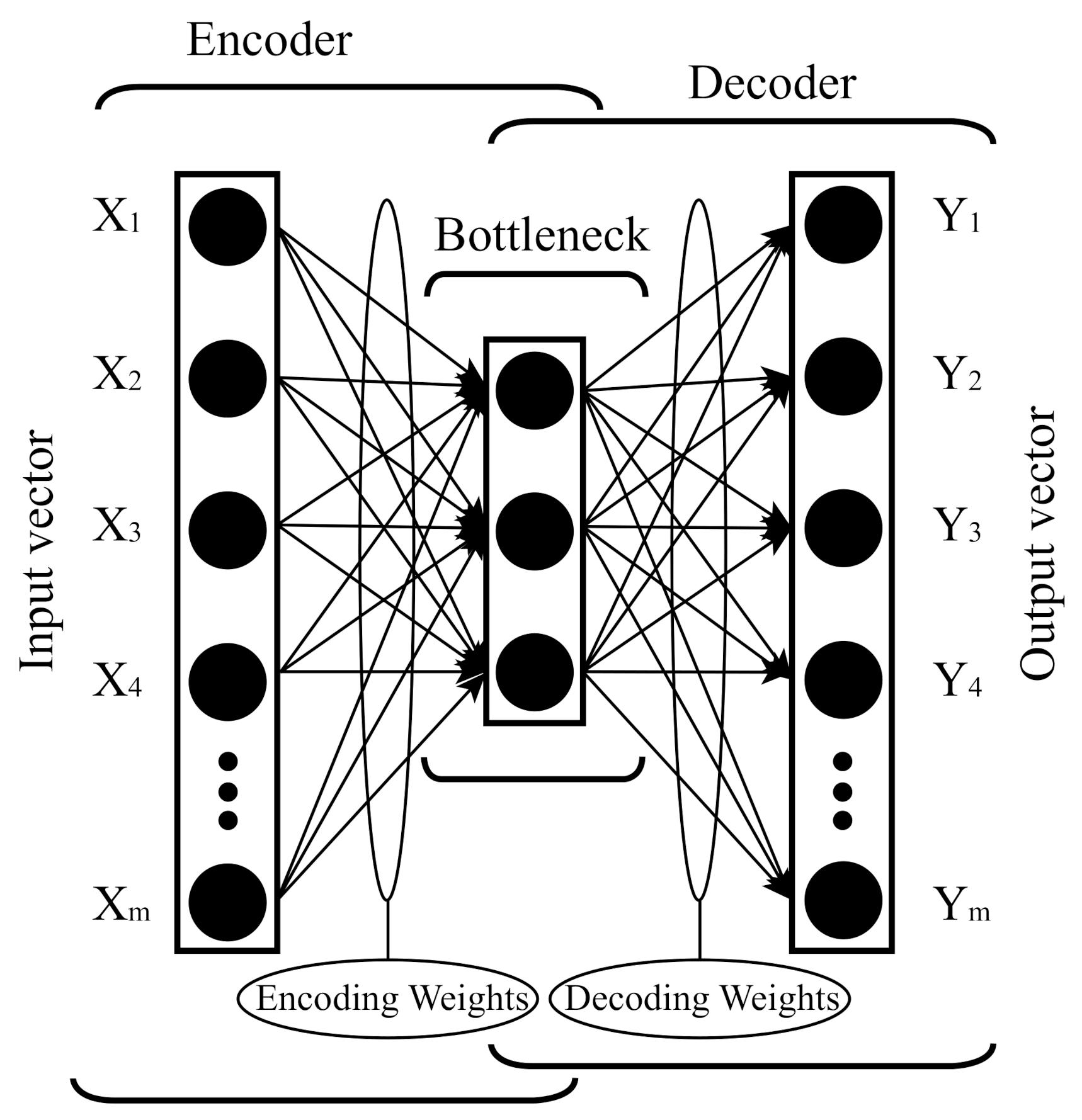
2.4. Pre-Training Concept

The primary nonlinear autoencoder is able to reduce the dimensionality in complex data, using its Bottleneck layer. The nonlinear autoencoder model was originally taken as a basis to generate early deep autoencoder architectures, where a cross-entropy error observed its optimization [15]. At present, a larger number of deep architectures are counted for [20], which efficiently discover subclasses in complex data. However, the strategy behind their success comes frequently from doing pre-training [21], leading to finding essential features in images, video, audio, and speech data in tasks for identification, classification, and reduction of memory. This concept is included in this paper for completeness.

2.5. Edge Computing Advantages by Using Neuromorphic Systems

The design of IoT devices and systems includes relevant advantages when the edge computing paradigm is delivered by Neuromorphic Systems (NS). We count the following.

• Energy efficiency: NS are more suitable than general-purpose computing hardware. The expected difference is several orders of magnitude.
• Low latency: NS surpass at processing continuous streams of data, reducing the delay to accomplish intelligent tasks.
• Adaptive processing: NS can adapt to changes in context.
• Rapid learning or adaptation: NS show capabilities beyond most standard artificial intelligence systems.

Extending this context, the spiking neural network presented in this work gives a basis for conceiving a neuromorphic processor prototype, whose advantages are below.

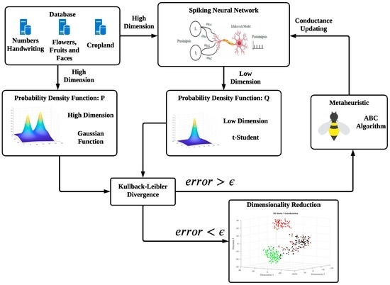
• The Artificial Bee Colony (ABC) algorithm is a gradient-free optimizer that conveniently replaces the STDP rule and backpropagation-based algorithms.
• The loss function in the t-distributed Stochastic Neighbor Embedding (t-SNE) method can act as the objective function in the ABC algorithm.
• The training phase is guided by the objective function of the ABC algorithm.
• The trained spiking neural network achieves efficiently a nonlinear dimensionality reduction, which is suitable for either task: reducing memory size or classifying complex data.

2.6. Metaheuristic Optimization

Optimal solutions in many complex engineering problems can be drawn from using metaheuristics methods, representing a practical alternative to gradient-based numerical procedures. Notably, the ABC algorithm [22] belongs to this optimization category. Its pseudocode is presented in Algorithm 1.

Algorithm 1 ABC Pseudocode.

1: Data: set control parameter values; 2: SN: Number of Food Sources, 3: MCN: Maximum Counter Number, 4: $limit:$ For deciding either a source is exhausted 5: Begin 6:  Initialize and evaluate the food source locations 7:  $counter=1$ 8:  while $counter<MCN$ do 9:    Employed Bees’ labor (see Algorithm 2) 10:    Onlooker Bees’ labor (see Algorithm 3) 11:    Memorize the Best Solution 12:    Scout Bees’ labor (see Algorithm 4) 13:    $counter++$ 14:  end while 15: End

In this pseudocode, the instructions named Employed Bees’ labor, Onlooker Bees’ labor, and Scout Bees’ labor follow the Algorithms 2–4, respectively, described in [23]. An employed bee randomly selects one food source $x_k$ from the current population and chooses a random dimension index j. The new food source is obtained by:

$$v_{ij}=x_{ij}+{\varphi }_{ij}\left(x_{ij}-x_{kj}\right),$$

(1)

where i is the solution currently being exploited, k is a randomly chosen neighbor solution, and ${\varphi }_{ij}$ is randomly chosen from $[-1,1]$ drawn from the uniform distribution. An employed bee unloads the nectar and then gives information to onlookers about the quality and the location of her source. High-quality solutions have a high chance to be selected but the solutions with low quality can also be selected by the onlookers [23]. The probability of each solution $\left(p_i\right)$ can be calculated proportionally to its fitness value:

$$p_i=\frac{fitnes{s}_i}{{\sum }_{i=1}^{SN}fitnes{s}_i}.$$

(2)

Algorithm 2 Employed Bees’ Labor Pseudocode (Modified from  [15]).

1: Data: food source population; 2: Begin 3:  for $foodsources<x_i$ do 4:   new solution $x{}^{\prime }\leftarrow producedbyEquation\left(1\right)$ 5:   $f\left(x{}^{\prime }\right)\leftarrow evaluatednewsolution$ 6:   if $f\left(x{}^{\prime }\right)<f\left(x_i\right)$ then 7:    $x_i\leftarrow x{}^{\prime }$ 8:    $exploit\left(x_i\right)\leftarrow 0$ 9:   else 10:    $exploit\left(x_i\right)\leftarrow exploit\left(x_i\right)+1$ 11:   end if 12:  end for 13: End

Algorithm 3 Onlooker Bees’ Labor Pseudocode (Modified from [15]).

1: Data: food source population; Probability of each solution 2: Begin 3:  for $food sources x_i$ do 4:   $p_i\leftarrow assignprobabilitybyEquation\left(2\right)$ 5:  end for 6:  $i\leftarrow 0$ 7:  $t\leftarrow 0$ 8:  while $t<SN$ do 9:   $r\leftarrow rand(0,1)$ 10:   if $r<p\left(i\right)$ then 11:     $t\leftarrow t+1$ 12:     $x_{}^{\prime }\leftarrow anewsolutionproducebyEquation\left(1\right)$ 13:     $f\left(x{}^{\prime }\right)\leftarrow evaluatenewsolution$ 14:     if $f\left(x{}^{\prime }\right)<f\left(x_i\right)$ then 15:     $x_i\leftarrow x{}^{\prime }$ 16:     $exploit\left(x_i\right)\leftarrow 0$ 17:     else 18:     $exploit\left(x_i\right)\leftarrow exploit\left(x_i\right)+1$ 19:     end if 20:   end if 21:   $i\leftarrow (i+1)mod(SN-1)$ 22:  end while 23: End

For a specific food source or solution X, if employed bees and onlooker bees cannot find any new food source or new solutions in its neighborhood to replace it, the food or solutions may be trapped into local minima. For this case, Scout Bees’ Labor must be applied.

Algorithm 4 Scout Bees’ Labor Pseudocode (Modified from [15]).

1: Data: food source population; Exploitation Counters 2: Begin 3:  $si=i:exploit\left(i\right)=max\left(exploit\right)$ 4:  if $exploit\left(si\right)>limit$ then 5:   $x_{si}\leftarrow randomsolutionbyEquation\left(1\right)$ 6:   $exploit\left(si\right)\leftarrow 0$ 7:  end if 8: End

2.7. The T-Sne Machine Learning Method

The t-distributed Stochastic Neighbor Embedding (t-SNE) [24] method was proposed as an alternative method for visualizing complex information in a reduced space or dimension, optimizing the quality of the clustering process to discover classes from data. It is successful due to its avoiding the “crowding-problem”, by both introducing a symmetrized cost function and using a t-distribution instead of a Gaussian one in the data. Although these changes favored using a stochastic gradient for the original optimization process, the resulting cost function also becomes suitable as the objective function for our experiments with the ABC algorithm. The below equation defines the objective function in this work. Its value is equal to the cross-entropy up to an additive constant.

$$C=KL\left(P\left|\right|Q\right)=\sum _i^{}\sum _j^{}{p}_{ij}log\frac{p_{ij}}{q_{ij}},$$

(3)

in this equation, KL(P||Q) is the Kullback-Leibler divergence between the joint distribution probability P in a high dimensionality space and the joint probability distribution Q in a low dimensionality space. The quantities $p_{ij}$ and $q_{ij}$ are the pairwise similarities in the low and high dimensionalities spaces, respectively. They are given with the Equations (4) and (5).

$$p_{ij}=\frac{exp\left(-{∥x_i-x_j∥}^2/2{\sigma }^2\right)}{{\sum }_{k\ne l}^{}exp\left(-{∥x_k-x_l∥}^2/2{\sigma }^2\right)},$$

(4)

$$q_{ij}=\frac{exp\left(-{∥y_i-y_j∥}^2\right)}{{\sum }_{k\ne l}^{}exp\left(-{∥y_k-y_l∥}^2\right)}.$$

(5)

3. Topics Related to Preparing Experiments

The next four subsections include succinct but relevant information for realizing the experiments, which generate the supporting results of the work.

3.1. Neuron Model Used in This Work

The spiking neuron model created by Izhikevich [25] takes advantage of other existing ones, due to its low-complexity numerical formulation. In addition, it reproduces with high accuracy the dynamic behavior of a biological neuron for a wide set of brain cortical tissues. It is widely accepted for designing computational neuromorphic hardware. We have used its dynamic differential equations, given below for producing another nonlinear spiking behavior, i.e., a sigmoidal response.

$$\begin{array}{cc}C\dot{v}=k\left(v-v_r\right)\left(v-v_t\right)-u+I& ifv\ge v_{peak},then\\ \dot{u}=a\left\{b\left(v-v_r\right)-u\right\}& v\leftarrow c,u\leftarrow u+d\end{array}$$

(6)

Table 1. Variables and parameters of the Izhikevich model.

Variables and Parameters	Name
v	membrane potential
u	membrane recovery
$v_r$	resting membrane potential
$v_t$	cutoff or threshold potential
C	membrane capacitance
I	injected current
$a,b,c,d,k$	dynamics type parameters

summarizes variables and parameters of the Izhikevich model.

Table 2. Typical values of principal configurations.

Neural Model Configurations (Acronym)	a	b	c	d
Regular Spiking (RS)	$0.02$	$0.2$	$-65$	8
Fast Spiking (FS)	$0.1$	$0.2$	$-65$	2
Low-Threshold Spiking (LTS)	$0.02$	$0.25$	$-65$	2
Chattering (CH)	$0.02$	$0.2$	$-50$	2
Intrinsically Bursting (IB)	$0.02$	$0.2$	$-55$	4

lists the values of the parameters a, b, c, and d of some of the main Izhikeivh neural model configurations, which are presented in a complementary publication by Izhikevich [26].

In particular, we find new and optimal values of the parameters: a, b, c, d, and k, to get a sigmoidal (or nonlinear) response in the rate of firing, which is achieved in a supervised manner and minimizing an MSE quantity.

Table 3. Values of a, b, c, d and k for sigmoidal response.

Name	Value
a	$-0.004811$ ms${}^{-1}$
b	$0.196783$
c	$-85.592772$ mV
d	$-5.343734$ mV
k	0.9
C	100 pF
$v_r$	$-60$ mV
$v_t$	$-40$ mV
$v_{peak}$	35 mV

, presents their values, which were found with the ABC algorithm. The values of other variables are also included.

In Figure 2, we can see the sigmoidal response of the spiking neuron as a nonlinear type configuration, where the parameters of Table 3 were used. The minimum and maximum Firing Rate (FR) values of the sigmoidal spiking neuron are 4 and 109 spikes/s, respectively, and, 4 and 104 for the reference continuous-sigmoid neuron. $70\times {10}^{-4}$ is the MSE value between these two graphs. To calculate the MSE value, the two graphs have been previously normalized dividing them by their respective maximum values of the firing rate.

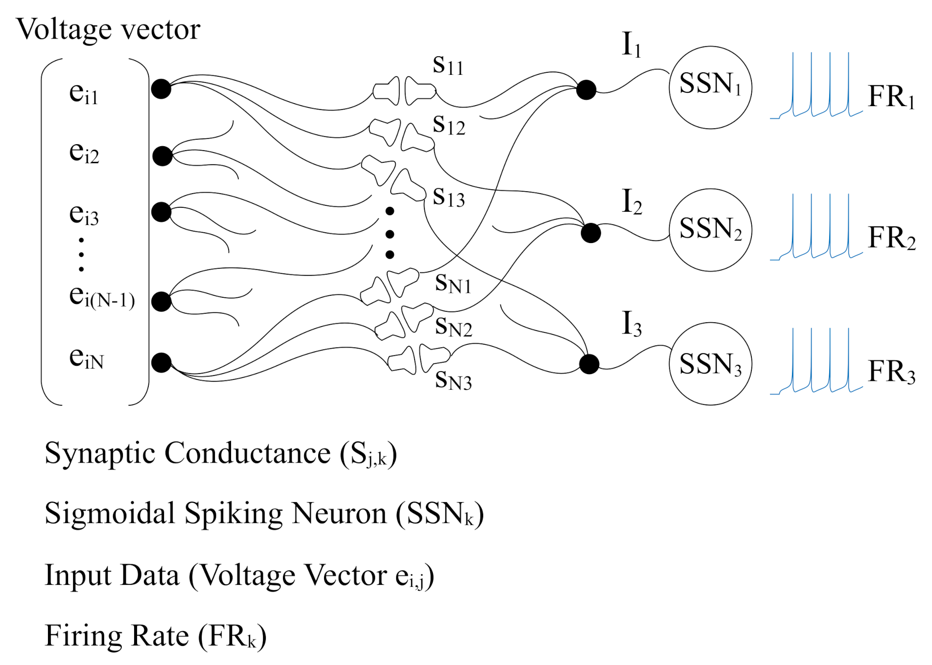
3.2. Spiking Neural Network Architecture Used in This Work

The architecture of the spiking neural network (SNN) for the experiments in this work is shown in Figure 3. There are 3 sigmoidal spiking neurons, i.e., $SS{N}_1$, $SS{N}_2$ and $SS{N}_3$, which generate spikes at Firing Rates in spikes/s: $F{R}_1$, $F{R}_2$ and $F{R}_3$, respectively. These neurons receive the electrical currents $I_1$, $I_2$ and $I_3$, which come from the set of transduced voltages $\left\{e_{i,j}\right\}$ by the set of conductances $\left\{s_{j,k}\right\}$.

3.3. Databases

In this work, three databases have been considered. The first one refers to the writing of numbers [27]. This was created considering the positions of the pixels on a Tablet with $500\times 500$ pixels, and the pressure values exerted by 44 writers when writing the numbers from 0 to 9. We have taken 1000 samples from this database and each sample is made up of 16 attributes.

The second database refers to a set of images of flowers, fruits and faces [28]. There are 100 images for each type. They are gray-scale images with a dimension of 100 rows by 100 columns. 67 characteristics have been extracted from each image, which corresponds to the coefficients of the Local Binary Pattern (LBP) image processing technique, with a processing block size of $64\times 64$.

The third database is a fused bi-temporal optical-radar data for cropland classification [29]. There are 98 radar features and 76 optical features, that is, each sample is made up of 174 features. Seven crop type classes exist for this data set as follows: 1—Corn; 2—Peas; 3—Canola; 4—Soybeans; 5—Oats; 6—Wheat; and 7—Broad-leaf.

Table 4. Database Parameters.

Name	Data	Features	Classes	Dimension
Handwriting Numbers	1000	16	10	$1000\times 16$
Fruits, Flowers, and Faces	300	67	3	$300\times 67$
Croplands	700	174	7	$700\times 174$

summarizes the parameters of the three database.

3.4. Training Phase Strategy

The SNN architecture depicted in Figure 3 has been arranged to play the encoding process of an autoencoder and from it, 3 Dimensions are synthesized. This represents a reduction in the dimensionality of the databases. This is equivalent to extracting the first three main components from each database. To understand the training phase for dimensionality reduction of the databases a flow diagram is presented in Figure 4.

The process starts by extracting from the input data a probability distribution function (PDF) named P, and this will be the reference for the search process, of the parameters corresponding to the synaptic conductances of three spiking neurons with the sigmoidal response. The SNN receives the data as a voltage vector and responds with an output matrix corresponding to the firing rate of each neuron.

The output matrix of the SNNs is considered as a possible dimensionality reduction of the data and from this process, a probability distribution function of the t-student type is obtained, named Q. The probability functions P and Q are compared to obtain their measure of similarity by calculating the Kullback-Leibler (K-L) divergence.

The K-L divergence is used as an objective function to be minimized by the ABC metaheuristic algorithm. The ABC algorithm is executed to determine the optimal values of the synaptic conductances. This process is repeatedly applied until reaching a certain $ϵ$ value, as a criterion for optimality of this process.

4. Experimental Results

This section presents the results of the dimensionality reduction task by the proposed spiking neural network. They come from three experiments, whose databases are named: Handwriting Numbers, Images, and Croplands. It is also included a discussion subsection.

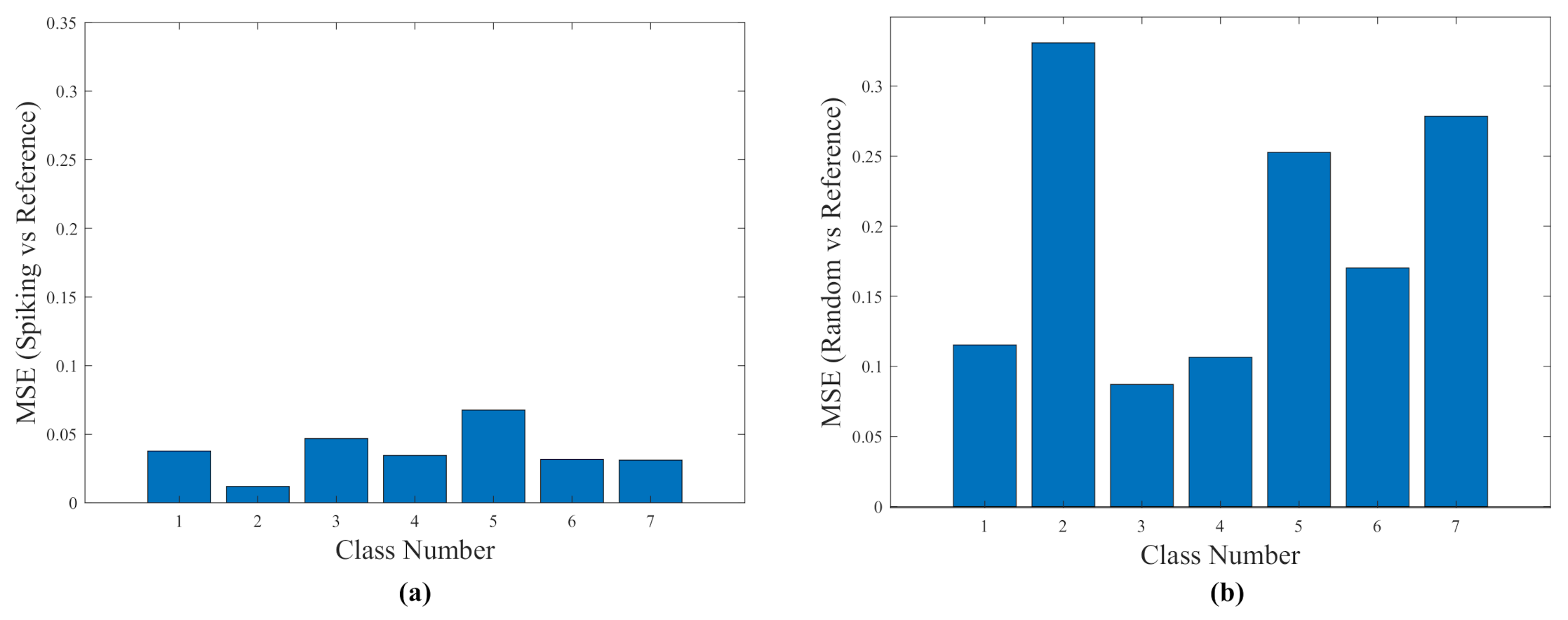
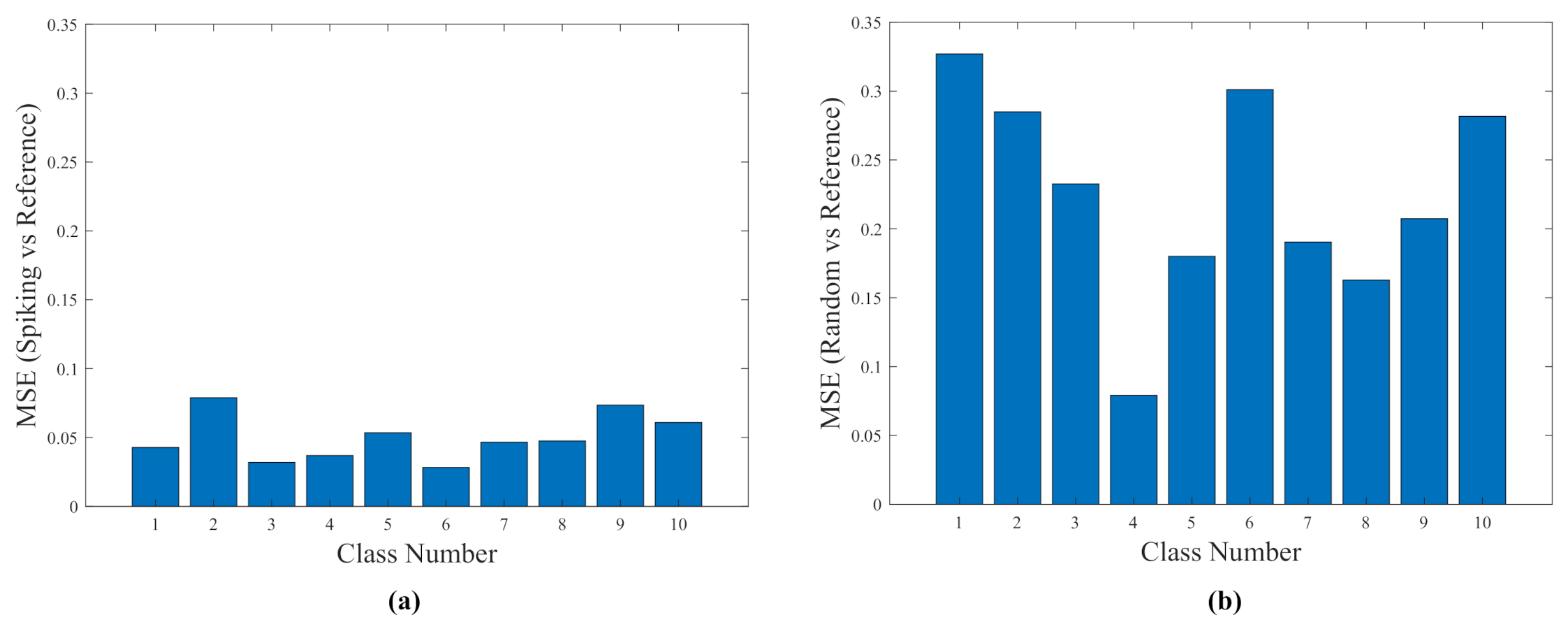
4.1. Relative Quality of Efficiency by Mse Evaluations

In principle, one spiking neural network can generate M output clusters from a set of input training vectors with M classes. In addition, each cluster will be visualized in a 3D space, whose 3 axes will be named Dimension 1, Dimension 2, and Dimension 3. The quality of this spiking neural network in performing the dimensionality reduction task over one class of M is evaluated with the MSE operator according to Equation (7).

$$MSE=\frac{1}{N}\times \sum {(D_{1,i}-D_{2,i})}^2,withi=1,\dots ,N,$$

(7)

The parameters in Equation $\left(7\right)$ are explained in

Table 5. Meaning of parameters.

Parameters
N, number of samples in one class.
{$D_{1,i}$}, set of distances between the center of the cluster and all N samples;
by a landmark experiment, in the same class.
{$D_{2,i}$}, set of distances between the center of the cluster and all N samples;
by the spiking network, in the same class.

, where there can be two landmark experiments, i.e., by $\left(1\right)$ a reference neural network and by $\left(2\right)$ a random numbers generator with uniform distribution. Case $\left(1\right)$ refers to a classic neural network with continuous-sigmoid neurons, replacing the spiking neurons. In case $\left(2\right)$, the distances come from a random function contained in a standard numerical platform.

From the above, we should realize two MSE quantifications for evaluating the quality of the spiking neural network.

• MSE-1: Spiking versus Reference. Measures the deviation of the spiking network versus a reference neural network.
• MSE-2: Random versus Reference. Measures the deviation of the random distances versus a reference neural network.

Comparing MSE-1 with MSE-2 is expected to get an MSE-1 lower than an MSE-2 to prove that the spiking neural network is able to correlate with the reference neural network. The adverse fact namely, MSE-1 equal to MSE-2, would show a lack of correlation.

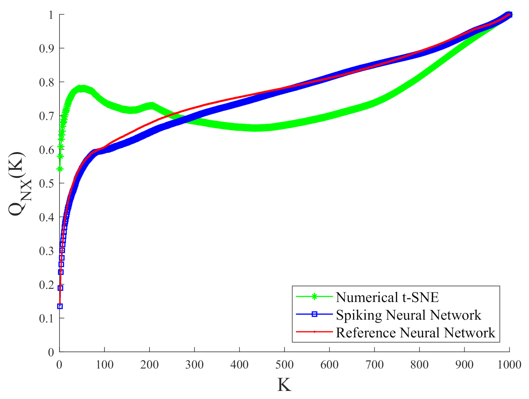
4.2. Quality Measurement by the Co-Ranking Matrix

Given the dimensionality reduction, the evaluation of the new data mapping about the data expressed in high dimensions remains to be completed. To determine this objective measurement, it is proposed to use the co-ranking matrix, introduced in [30] and defined as

$$Q_{kl}=\left|\left\{(i,j)|{\rho }_{ij}=kand{r}_{ij}=l\right\}\right|,$$

(8)

where ${\rho }_{ij}$ represents the rank of $x_i$ with respect to $x_j$ in the high-dimensional space of the original database. For its part, $r_{ij}$ is the rank of $y_i$ with respect to $y_j$ in the proposed low-dimensional space, and $\left|·\right|$ denotes the number of elements in the set. The ranks are calculated using Equation (9), where ${\delta }_{ij}$ represents the distance from $x_i$ to $x_j$ while $d_{ij}$ goes from $y_i$ to $y_j$:

$$\begin{array}{c}{\rho }_{ij}=\left|\left\{k|{\delta }_{ik}<{\delta }_{ij}or\left({\delta }_{ik}={\delta }_{ij}andk<j\right)\right\}\right|\\ r_{ij}=\left|\left\{k|d_{ik}<d_{ij}or\left(d_{ik}=d_{ij}andk<j\right)\right\}\right|\end{array}.$$

(9)

When the values in the co-ranking matrix are set on the main diagonal, it is interpreted that the mapping is perfect. Although this quotation is almost impossible to fulfill for original data, the measurements themselves suffer from slight variations, causing alterations interpreted as intrusions or extrusions. An intrusion is considered when a point j has a lower rank with respect to the point i, in the representation of low-dimensional data compared to high-dimensional data. Conversely, an extrusion occurs when a point j has a higher rank with respect to point i in low-dimensional representation compared to high-dimensional data.The intrusion points are located below the main diagonal; the extrusion points above.

An improvement in the calculation of the co-ranking matrix is presented in [31]. The quality of the representation of low-dimensional data is measured as a function of the number of points that remain within a k-neighborhood during the projection process.To carry out this measurement, we will use Equation (10), where N represents the number of total points and K ends the value of the neighborhood:

$$Q_{NX}\left(K\right)=\frac{1}{KN}\sum _{k=1}^K\sum _{l=1}^K{Q}_{kl}.$$

(10)

$Q_{NX}\left(K\right)$ is sensible for a small number of samples, where the mapping error might become large. In addition, over a particular value of K, the error saturates to a low value. The relation $Q_{NX}\left(K\right)$ versus the number of samples is a curve that follows a diagonal, where it represents the ideal $Q_{NX}\left(K\right)$. The expected quality comes from the numerical $Q_{NX}\left(K\right)$ graph, where it saturates. The saturation point is identified where the ranking matrix starts to follow the main diagonal. We will evaluate the dimensionality reduction task visually. We will compare saturations in both numerical and experimental curves.

4.3. Handwriting Numbers Experiment

To determine the performance of the spiking neural network in reducing dimensionality, its result has been compared with the response obtained with a reference neural network built with continuous-sigmoid neurons. The three databases have been evaluated with both architectures and the results are presented below.

Figure 5 shows the dimensionality reduction obtained with the two architectures when the database corresponds to handwriting numbers. In Figure 5a, the distribution of the 10 classes granted by the SNN is shown. In Figure 5b, the distribution of the classes with reference neural network is shown. In Figure 5c, the distribution of the class corresponding to digit zero is shown. In blue color, the SNN distribution is shown, and black color, the reference continuous-sigmoid neural network distribution is shown. The process is repeated similarly way for the rest of the classes and they are graphed in Figure 5d–l.

The response of each neuron, namely with spiking and continuous neurons, is considered as a dimension in the graphs of Figure 5. The values of the centers of the classes for each dimension are presented in Figure 6. From these graphs, it is observed the high similarity in the response of both networks.

As it was stated in Section 4.1, and for evaluating the quality of the dimensionality reduction task in this experiment, i.e., Handwriting Numbers Experiment, we calculate the quantities MSE-1 and MSE-2. They are presented in Figure 7.

As mentioned in Section 4.2, to evaluate the quality of the data representation in low dimensions, the calculation of the co-ranking matrix has been obtained. Figure 8 contains the graphs of the co-ranking matrix, which corresponds to the dimension reduction of the database of handwritten numbers, for three techniques, numerical t-SNE, Spiking Neural Network, and Reference Neural Network.

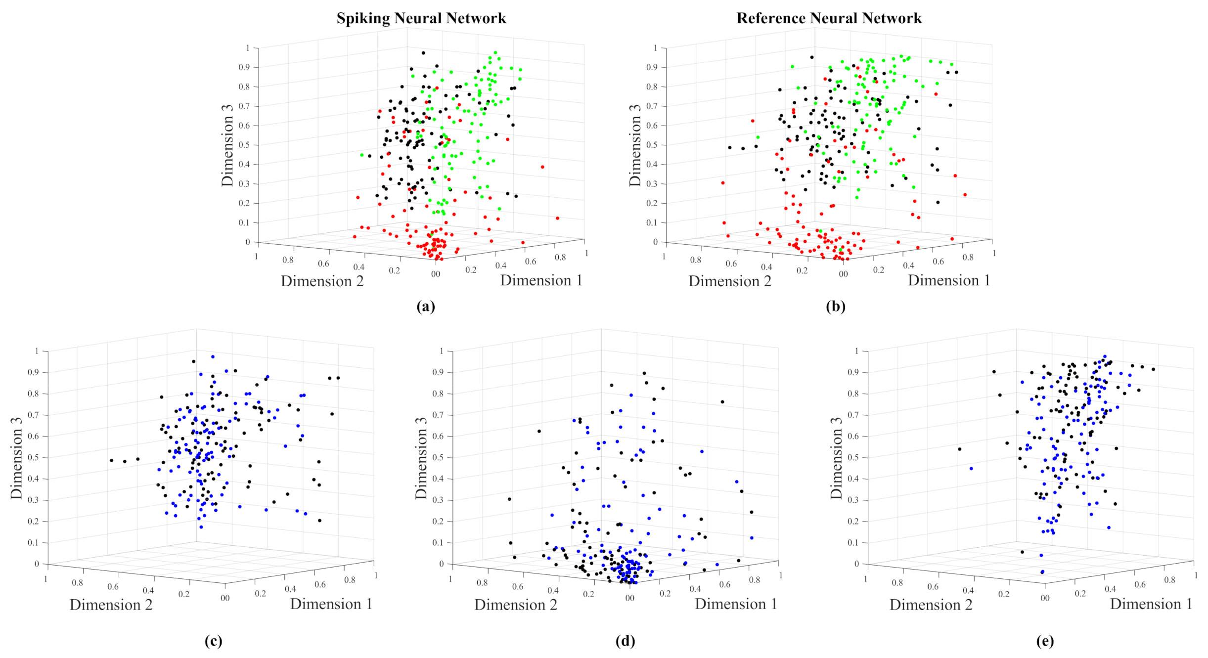
4.4. Images Experiment

In this experiment, the database contains 3 classes of gray-scale images, i.e., Flowers, Fruits, and Human Faces. As it has proceeded in Section 4.3, we also do the same to show the dimensionality reduction result by both the SNN and the reference neural network in Figure 9a,b. This figure also includes the classes separately, from Figure 9c–e.

Figure 10 shows the dimensions of the centers of the classes of both networks namely, the SNN and the reference neural network. We observe that both networks generate similar distributions.

As it was stated in Section 4.3, and for evaluating the quality of the dimensionality reduction task in this experiment, i.e., Images Experiment, we calculate the quantities MSE-1 and MSE-2. They are presented in Figure 11.

In order to evaluate the quality of the representation of the data in low dimensions, the calculation of the co-ranking matrix has been obtained. Figure 12 contains the graphs of the co-ranking matrix for the database comprised of images of Flowers, Fruits, and Faces. Three techniques have been evaluated, numerical t-SNE, Spiking Neural Network, and Reference Neural Network.

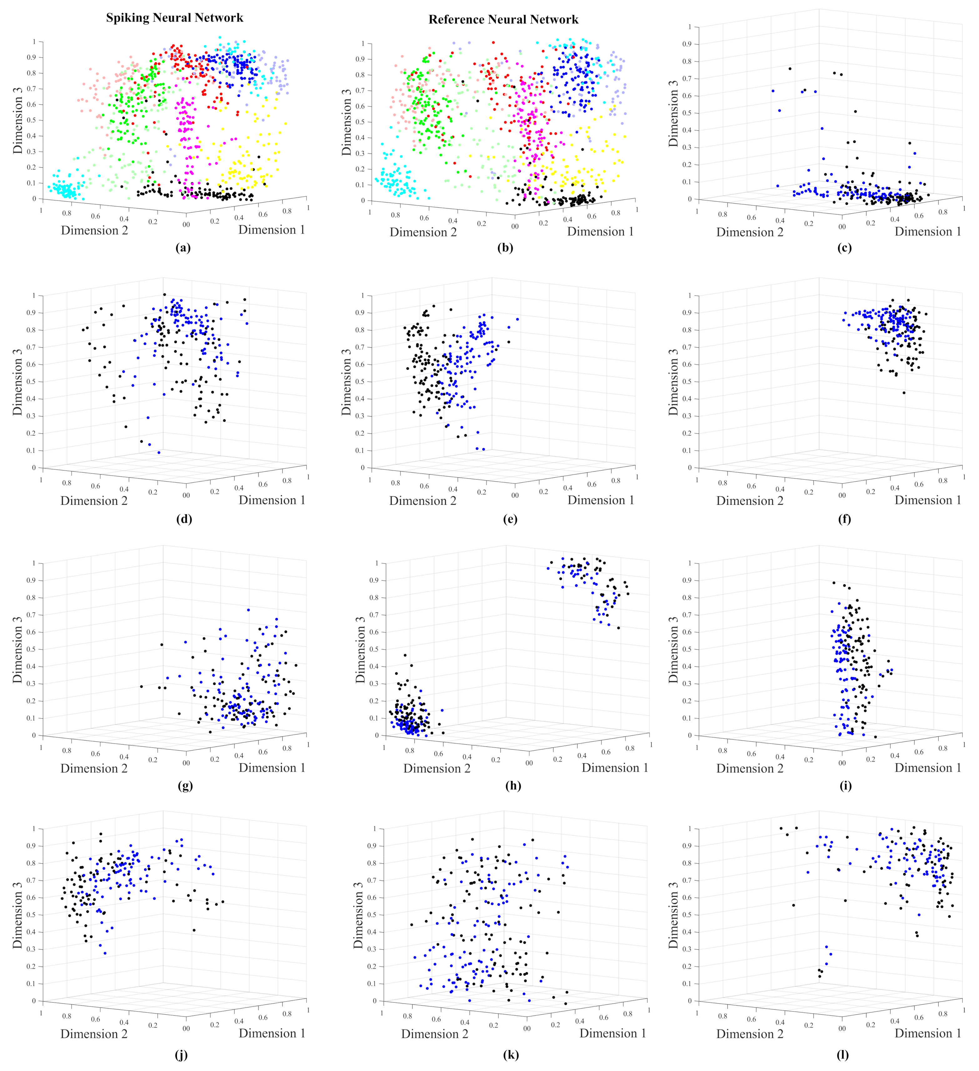
4.5. Croplands Experiment

In this experiment, the database contains seven classes of complex data related to croplands, i.e., corn, peas, canola, soybeans, oats, wheat, and broad-leaf. As has proceeded in Section 4.3, we also do the same to show the dimensionality reduction result by both the SNN and the reference neural network in Figure 13a,b, respectively. This figure also includes the classes separately, from Figure 13c–i.

The values of the centers of the classes for each dimension are presented in Figure 14. We observe that both networks generate similar distributions.

As it was stated in Section 4.1, and for evaluating the quality of the dimensionality reduction task in this experiment, i.e., Croplands Experiment, we calculate the quantities MSE-1 and MSE-2. They are presented in Figure 15.

In order to evaluate the quality of the representation of the data in low dimensions, the calculation of the co-ranking matrix has been obtained. Figure 16 contains the graphs of the co-ranking matrix for the database that referer to cropland. Three techniques have been evaluated, numerical t-SNE, Spiking Neural Network, and Reference Neural Network.

4.6. Discussion

In the machine learning community, a fair evaluation of any dimensionality reduction method would require knowing the reconstruction error that uses some available inverse mapping process. In our case, this is not possible for the moment. Alternatively, we consider three standard techniques for the evaluation, using a visual data method and two quality functions, MSE and co-ranking matrices. The four points below argue these evaluations on the results:

• The visual data method can be applied in Figure 5, Figure 9, and Figure 13. The deduction drawn is that all they are coherent.
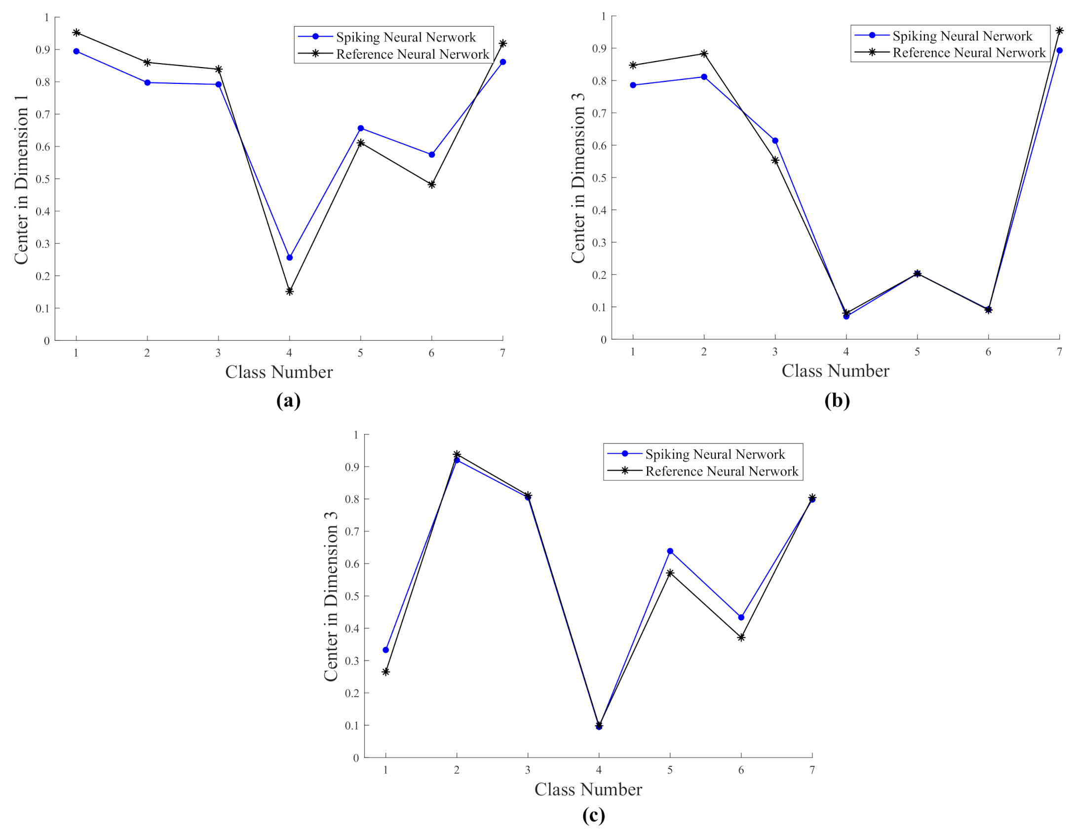
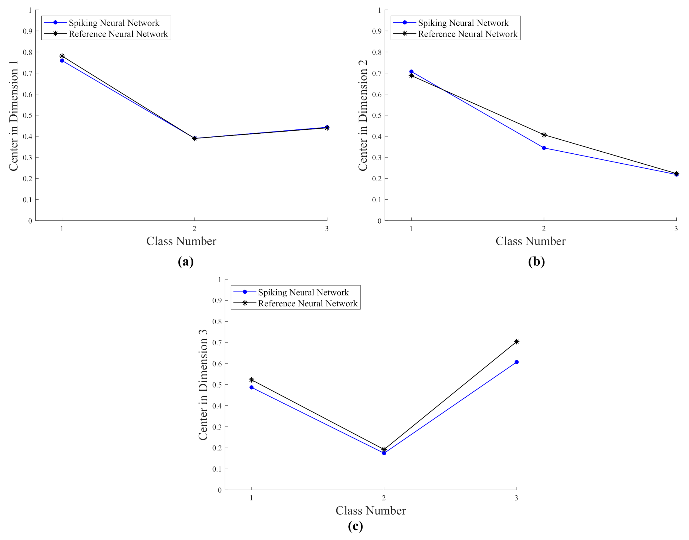
• The numerical evaluation of the centers of the classes, i.e., Dimension 1, Dimension 2, and Dimension 3 in Figure 6, Figure 10, and Figure 14, by both the reference and spiking networks follow the same trend pattern. This proves that the spiking networks reproduce a performance near to the reference network.
• The MSE-1 and MSE-2 values are reported graphically in Figure 7, Figure 11, and Figure 15 and, whose comparisons follow the premises, P1 and P2. Their statements are below.
  • P1. MSE-1 can compare the results provided by the experimental spiking network with the set of the expected results produced by a continuous sigmoid neuron network. MSE-1 should be relatively small.
  • P2. MSE-2 can compare the results provided by a no correlated network with the set of the expected results produced by a continuous sigmoid neuron network. MSE-2 should be relatively large.
  Comparing MSE-1 with MSE-2 leads to find that MSE-1 is always lower than MSE-2. This point proves that the efficiencies by all the SNNs are acceptable.
• The graphical results in Figure 8, Figure 12, and Figure 16 show co-ranking matrices for all the experiments. The pairs Spiking/Reference Network have nearly the same trace. In addition, the third trace due to the numeric t-SNE was presented as the theoretical case, whose saturation is the same as the spiking and reference networks. The evaluation at this point demonstrates that the quality of the spiking networks are satisfactory.

The above 4 points show that the spiking neural networks in this article have a suitable performance in the nonlinear dimensionality reduction task.

The works [6,7,8,9,10,11,12] cited in the Introduction section about training spiking systems through using metaheuristics focus on either improving the backpropagation type algorithm or demonstrating the performance of evolutionary algorithms do not get concerned with using another objective function from artificial intelligence theory, but the fundamental MSE estimator. For completeness, we mention alternative and recent strategies to create spiking systems that include transforming continuous deep neural systems into spiking systems [32], using particular training formulations which compare superb with the SpikeProp algorithm but associated with particular loss function [33], retaking the biological STDP rule for convolutional deep networks [34], tuning convolutional-type networks with a biologically plausible algorithm [35], to name a few.

An extension of this experimental work would include more databases in number and attributes to categorize the efficiency of the intelligent capability of our spiking networks.

5. Conclusions

The spiking neural network paradigm is becoming suitable for implementing in hardware intelligent tasks. Therefore, these systems would have advantages derived from neuromorphic schemes. However, the training method for establishing efficiently the weighting values of the synaptic connection between neurons is still an open issue. In this work, we have presented meaningful results proving that the ABC algorithm is capable to solve this complex task. The reason for the efficiency in this metaheuristic algorithm is due to its capability to leave local minima, which certainly leads to find optimal solutions.

The problem conducted in this paper is related to reduce the nonlinear dimensionality of complex databases, which was realized with the proposed spiking neural network using available or generated attributes of the data. The nonlinearity transformation from high to low dimensions was implemented with sigmoidal spiking neurons, which were created also with the ABC algorithm. The loss function defined in the t-SNE method served as the objective function in the ABC algorithm, keeping its original properties on the user data during the training phase of the spiking neural network.

The intelligent process performed with the trained spiking neural network in this work is still partial. It needs a further spiking softmax network for evaluating numerically the actual classes.

References

1. Luo, W.; Lu, J.; Li, X.; Chen, L.; Liu, K. Rethinking Motivation of Deep Neural Architectures. IEEE Circuits Syst. Mag. 2020, 20, 65–76. [Google Scholar] [CrossRef]
2. Roy, K.; Jaiswal, A.; Panda, P. Towards spike-based machine intelligence with neuromorphic computing. Nature 2019, 575, 607–617. [Google Scholar] [CrossRef]
3. Wang, X.; Lin, X.; Dang, X. Supervised learning in spiking neural networks: A review of algorithms and evaluations. Neural Netw. 2020, 125, 258–280. [Google Scholar] [CrossRef] [PubMed]
4. Bouvier, M.; Valentian, A.; Mesquida, T.; Rummens, F.; Reyboz, M.; Vianello, E.; Beigne, E. Spiking neural networks hardware implementations and challenges: A survey. Acm J. Emerg. Technol. Comput. Syst. (JETC) 2019, 15, 1–35. [Google Scholar] [CrossRef]
5. Ojha, V.K.; Abraham, A.; Snášel, V. Metaheuristic design of feedforward neural networks: A review of two decades of research. Eng. Appl. Artif. Intell. 2017, 60, 97–116. [Google Scholar] [CrossRef] [Green Version]
6. Vazquez, R.A. Training spiking neural models using cuckoo search algorithm. In Proceedings of the 2011 IEEE Congress of Evolutionary Computation (CEC), New Orleans, LA, USA, 5–8 June 2011; pp. 679–686. [Google Scholar]
7. Vazquez, R.A.; Garro, B.A. Training spiking neural models using artificial bee colony. Comput. Intell. Neurosci. 2015, 2015, 947098. [Google Scholar] [CrossRef] [PubMed] [Green Version]
8. Enríquez-Gaytán, J.; Gómez-Castañeda, F.; Flores-Nava, L.; Moreno-Cadenas, J. Spiking neural network approaches PCA with metaheuristics. Electron. Lett. 2020, 56, 488–490. [Google Scholar] [CrossRef]
9. Pavlidis, N.; Tasoulis, O.; Plagianakos, V.P.; Nikiforidis, G.; Vrahatis, M. Spiking neural network training using evolutionary algorithms. In Proceedings of the Proceedings, 2005 IEEE International Joint Conference on Neural Networks, Montreal, QC, Canada, 31 July–4 August 2005; Volume 4, pp. 2190–2194. [Google Scholar]
10. Altamirano, J.S.; Ornelas, M.; Espinal, A.; Santiago-Montero, R.; Puga, H.; Carpio, J.M.; Tostado, S. Comparing Evolutionary Strategy Algorithms for Training Spiking Neural Networks. Res. Comput. Sci. 2015, 96, 9–17. [Google Scholar] [CrossRef]
11. López-Vázquez, G.; Ornelas-Rodriguez, M.; Espinal, A.; Soria-Alcaraz, J.A.; Rojas-Domínguez, A.; Puga-Soberanes, H.; Carpio, J.M.; Rostro-Gonzalez, H. Evolutionary spiking neural networks for solving supervised classification problems. Comput. Intell. Neurosci. 2019, 2019, 4182639. [Google Scholar] [CrossRef]
12. Liu, C.; Shen, W.; Zhang, L.; Du, Y.; Yuan, Z. Spike Neural Network Learning Algorithm Based on an Evolutionary Membrane Algorithm. IEEE Access 2021, 9, 17071–17082. [Google Scholar] [CrossRef]
13. Jolliffe, I.T.; Cadima, J. Principal component analysis: A review and recent developments. Philos. Trans. R. Soc. A Math. Phys. Eng. Sci. 2016, 374, 20150202. [Google Scholar] [CrossRef]
14. Ji, S.; Wuang, Z.; Wei, Y. Principal Component Analysis and Autoencoders. Available online: http://people.tamu.edu/~sji/classes/PCA.pdf (accessed on 22 April 2021).
15. Hinton, G.E.; Salakhutdinov, R.R. Reducing the dimensionality of data with neural networks. Science 2006, 313, 504–507. [Google Scholar] [CrossRef] [Green Version]
16. Asghari, P.; Rahmani, A.M.; Javadi, H.H.S. Internet of Things applications: A systematic review. Comput. Netw. 2019, 148, 241–261. [Google Scholar] [CrossRef]
17. Shi, W.; Cao, J.; Zhang, Q.; Li, Y.; Xu, L. Edge computing: Vision and challenges. IEEE Internet Things J. 2016, 3, 637–646. [Google Scholar] [CrossRef]
18. Al-Garadi, M.A.; Mohamed, A.; Al-Ali, A.K.; Du, X.; Ali, I.; Guizani, M. A survey of machine and deep learning methods for internet of things (IoT) security. IEEE Commun. Surv. Tutor. 2020, 22, 1646–1685. [Google Scholar] [CrossRef] [Green Version]
19. Zhou, Z.; Chen, X.; Li, E.; Zeng, L.; Luo, K.; Zhang, J. Edge intelligence: Paving the last mile of artificial intelligence with edge computing. Proc. IEEE 2019, 107, 1738–1762. [Google Scholar] [CrossRef] [Green Version]
20. Nielsen, M.A. Neural Networks and Deep Learning; Determination Press: San Francisco, CA, USA, 2015; Volume 25. [Google Scholar]
21. Erhan, D.; Courville, A.; Bengio, Y.; Vincent, P. Why does unsupervised pre-training help deep learning? In Proceedings of the Thirteenth International Conference on Artificial Intelligence and Statistics, JMLR Workshop and Conference Proceedings, Sardinia, Italy, 13–15 May 2010; pp. 201–208. [Google Scholar]
22. Karaboga, D.; Basturk, B. On the performance of artificial bee colony (ABC) algorithm. Appl. Soft Comput. 2008, 8, 687–697. [Google Scholar] [CrossRef]
23. Bennis, F.; Bhattacharjya, R.K. Nature-inspired Methods for Metaheuristics Optimization: Algorithms and Applications in Science and Engineering; Springer: Berlin/Heidelberg, Germany, 2020; Volume 16. [Google Scholar]
24. Van der Maaten, L.; Hinton, G. Visualizing data using t-SNE. J. Mach. Learn. Res. 2008, 9, 2579–2605. [Google Scholar]
25. Izhikevich, E.M. Dynamical Systems in Neuroscience; MIT Press: Cambridge, MA, USA, 2007. [Google Scholar]
26. Izhikevich, E.M. Simple model of spiking neurons. IEEE Trans. Neural Netw. 2003, 14, 1569–1572. [Google Scholar] [CrossRef] [PubMed] [Green Version]
27. Handwritten Digits Data Set. Available online: https://archive.ics.uci.edu/ml/datasets/Pen-Based+Recognition+of+Handwritten+Digits (accessed on 29 April 2021).
28. Flowers, Fruits and Faces Data Set. Available online: https://es.dreamstime.com/foto-de-archivo-sistema-de-caras-de-la-gente-image79273852 (accessed on 22 April 2021).
29. Fused Optical-Radar Data Set. Available online: https://archive.ics.uci.edu/ml/datasets/Crop+mapping+using+fused+optical-radar+data+set# (accessed on 29 April 2021).
30. Lee, J.A.; Verleysen, M. Quality assessment of dimensionality reduction: Rank-based criteria. Neurocomputing 2009, 72, 1431–1443. [Google Scholar] [CrossRef]
31. Lueks, W.; Mokbel, B.; Biehl, M.; Hammer, B. How to evaluate dimensionality reduction?—Improving the co-ranking matrix. arXiv 2011, arXiv:1110.3917. [Google Scholar]
32. Xu, Y.; Tang, H.; Xing, J.; Li, H. Spike trains encoding and threshold rescaling method for deep spiking neural networks. In Proceedings of the 2017 IEEE Symposium Series on Computational Intelligence (SSCI), Honolulu, HI, USA, 27 November–1 December 2017; pp. 1–6. [Google Scholar]
33. Mostafa, H. Supervised learning based on temporal coding in spiking neural networks. IEEE Trans. Neural Netw. Learn. Syst. 2017, 29, 3227–3235. [Google Scholar] [CrossRef] [Green Version]
34. Lee, C.; Srinivasan, G.; Panda, P.; Roy, K. Deep spiking convolutional neural network trained with unsupervised spike-timing-dependent plasticity. IEEE Trans. Cogn. Dev. Syst. 2018, 11, 384–394. [Google Scholar]
35. Zhang, T.; Jia, S.; Cheng, X.; Xu, B. Tuning Convolutional Spiking Neural Network With Biologically Plausible Reward Propagation. IEEE Trans. Neural Netw. Learn. Syst. 2021. [Google Scholar] [CrossRef]
Figure 1. Architecture of the Autoencoder.
Electronics 10 01679 g001
Figure 2. Response of spiking neuron in sigmoidal configuration (Nonlinear Response).
Electronics 10 01679 g002
Figure 3. Spiking Neural Network Architecture.
Electronics 10 01679 g003
Figure 4. Training Process of the Spiking Neural Network.
Electronics 10 01679 g004
Figure 5. Class distribution for the Handwriting Numbers Database. In Figure 5a,b, each color represents a class. In Figure 5c–l the blue color corresponds to the SNN distribution and the black color to the reference continuous-sigmoid neural network distribution. (b) Distribution from Autoencoder. (c) Number “zero”. (d) Number “one”. (e) Number “two”. (f) Number “three”. (g) Number “four”. (h) Number “five”. (i) Number “six”. (j) Number “seven”. (k) Number “eight”. (l) Number “nine”.
Electronics 10 01679 g005
Figure 6. Values of centers. (a) Value of Centers in Dimension 1. (b) Value of Centers in Dimension 2. (c) Value of Centers in Dimension 3.
Electronics 10 01679 g006
Figure 7. MSE values. (a) MSE-1: Spiking versus Reference. (b) MSE-2: Random versus Reference.
Electronics 10 01679 g007
Figure 8. The graphs of the co-ranking matrix.
Electronics 10 01679 g008
Figure 9. Class distribution for the Flowers, Fruits and Faces Database. In Figure 9a,b, each color represents a class. In Figure 9c–e the blue color corresponds to the SNN distribution and the black color to the reference continuous-sigmoid neural network distribution. (a) Distribution from SNN architecture. (b) Distribution from autoencoder. (c) Flowers class. (d) Fruit class. (e) Faces class.
Electronics 10 01679 g009
Figure 10. Values of Centers. (a) Value of Centers in Dimension 1. (b) Value of Centers in Dimension 2. (c) Value of Centers in Dimension 3.
Electronics 10 01679 g010
Figure 11. MSE values. (a) MSE-1: Spiking versus Reference. (b) MSE-2: Random versus Reference.
Electronics 10 01679 g011
Figure 12. The graphs of the co-ranking matrix.
Electronics 10 01679 g012
Figure 13. Class distribution for the Cropland Database. In Figure 13a,b, each color represents a class. In Figure 13c–i the blue color corresponds to the SNN distribution and the black color to the reference continuous-sigmoid neural network distribution. (a) Distribution from SSN architecture. (b) Distribution from Reference Continuous Neuron. (c) Corn class. (d) Peas class. (e) Canola class. (f) Soybeans class. (g) Oats class. (h) Wheat class. (i) Broad-Leaf class.
Electronics 10 01679 g013
Figure 14. Values of Centers. (a) Value of Centers in Dimension 1. (b) Value of Centers in Dimension 2. (c) Value of Centers in Dimension 3.
Electronics 10 01679 g014
Figure 15. MSE values. (a) MSE-1: Spiking versus Reference. (b) MSE-2: Random versus Reference.
Electronics 10 01679 g015
Figure 16. The graphs of the co-ranking matrix.
Electronics 10 01679 g016