Modeling and Prediction of Daily Traffic Patterns—WASK and SIX Case Study

Abstract

The paper studies efficient modeling and prediction of daily traffic patterns in transport telecommunication networks. The investigation is carried out using two historical datasets, namely WASK and SIX, which collect flows from edge nodes of two networks of different size. WASK is a novel dataset introduced and analyzed for the first time in this paper, while SIX is a well-known source of network flows. For the considered datasets, the paper proposes traffic modeling and prediction methods. For traffic modeling, the Fourier Transform is applied. For traffic prediction, two approaches are proposed—modeling-based (the forecasting model is generated based on historical traffic models) and machine learning-based (network traffic is handled as a data stream where chunk-based regression methods are applied for forecasting). Then, extensive simulations are performed to verify efficiency of the approaches and their comparison. The proposed modeling method revealed high efficiency especially for the SIX dataset, where the average error was lower than 0.1%. The efficiency of two forecasting approaches differs with datasets–modeling-based methods achieved lower errors for SIX while machine learning-based for WASK. The average prediction error for SIX reached 3.36% while forecasting for WASK turned out extremely challenging.

1. Introduction

The beginnings of transport telecommunication networks date back to the 1960s, when the ARPA (Advanced Research Project Agency) established the first wide area network called ARPANET (ARPA Network). Initially, ARPANET was a simple packet forwarding network connecting only two computers. However, due to its invaluable usefulness and work facilitation, it has been rapidly developed and today it is known as the Internet precursor [1]. Currently, telecommunication networks are an indispensable part of the society’s everyday life, providing support for plenty of our activities—education, business, health care, finance, social life, entertainment, etc. The extremely relevant role of networks in our life was also revealed and emphasized during the COVID-19 pandemic, when many important human activities (e.g., business, education) could only be realized remotely [2]. The networks’ immensely relevant position in our society entails the continuous growth of the number of network users and connected devices as well as their increasing requirements regarding the networks [3]. According to Cisco company, there will be 5.3 billion total Internet users (66% of global population) by 2023, up from 3.9 billion (51% of global population) in 2018, and there will be 29.3 billion networked devices by 2023 up from 18.4 billion in 2018. Moreover, the bandwidth demands of the most popular services (for instance video) will increase up to several times [3].

Increasing requirements regarding networks and constantly growing traffic trigger the fast development and implementation of new network architectures and technologies [4]. The new solutions benefit from advance transmission and spectrum management techniques (for instance, adaptive application of complex modulation formats and continuous monitoring of links/paths QoS parameters) [5]. In turn, they are able to provide superior network performance. However, at the cost of complex network design and operational optimization. Therefore, the adoption of these innovations entails an urgent need for improvement in the field of network design and optimization algorithms, which can be achieved either by revisiting existing methods or by completely new proposals [4,6].

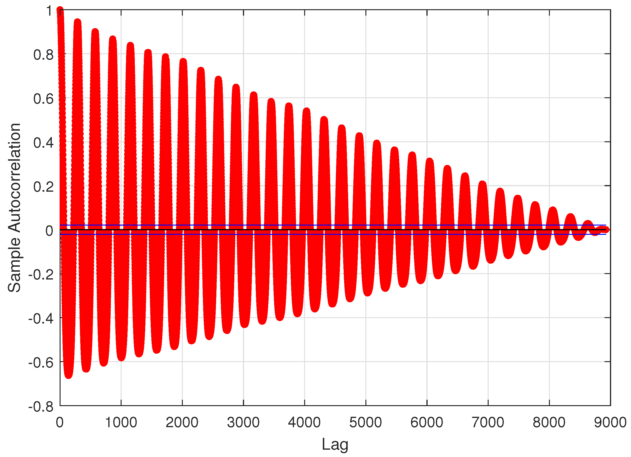
The results of recent research in the field of networking have revealed a promising direction in the algorithms improvement—design and implementation of traffic-aware methods [4]. In more detail, the network traffic is not a random process and it follows specific patterns, which come from human behaviours as a result of working habits, weekend activities, and so on [7,8,9]. It was observed that the more aggregated the traffic is (from a higher number of users), the more regular its shape is as a time function and the patterns are more noticeable. The main idea of the traffic-based approach is to collect information regarding observed traffic flows in networks and then to apply various modeling approaches or/and machine learning algorithms to process that data and extract hidden patterns [4]. The patterns might be then utilized to predict future traffic and use it to design and optimize network performance [10]. The crucial element of the traffic-aware approach is to collect a vast set of representative data, which might be difficult due to the privacy and security reasons, and properly select a beneficial modeling/prediction method depending on the data characteristics [4].

The traffic-aware methods might benefit from short-term or the long-term traffic forecasting [4]. In the short-term prediction, the traffic forecast is made for the near future, i.e., for a period up to several upcoming time stamps (typically only for the next time stamp). That information may be then utilized for instance to plan the routing rules for the approaching traffic demands. By these means, it is possible to increase the ratio of the accepted demands while a demand switching process is realized faster [11,12]. In the long-term prediction, which is much more challenging, the forecast is made for a longer period (i.e., several upcoming hours or even days/months). That information might be then used by the network operators to precisely plan the resources’ (i.e., computing and networking infrastructure) assignment process for the forthcoming requests in such a way as to obtain numerous benefits. For instance, in order to: (i) maximize the number of served clients, (ii) maximize their quality of service, (iii) improve the resource utilization, and (iv) reduce the power consumption (which meets the green networking paradigm) [4,13,14]. The long-term traffic forecasting improves also the increasingly popular model of the resource outsourcing. In that model, a client who does not have their own computing/networking resources, can outsource it from an external company. To this end, the client must define their requirements, what might be realized by analyzing the long-term traffic forecast.

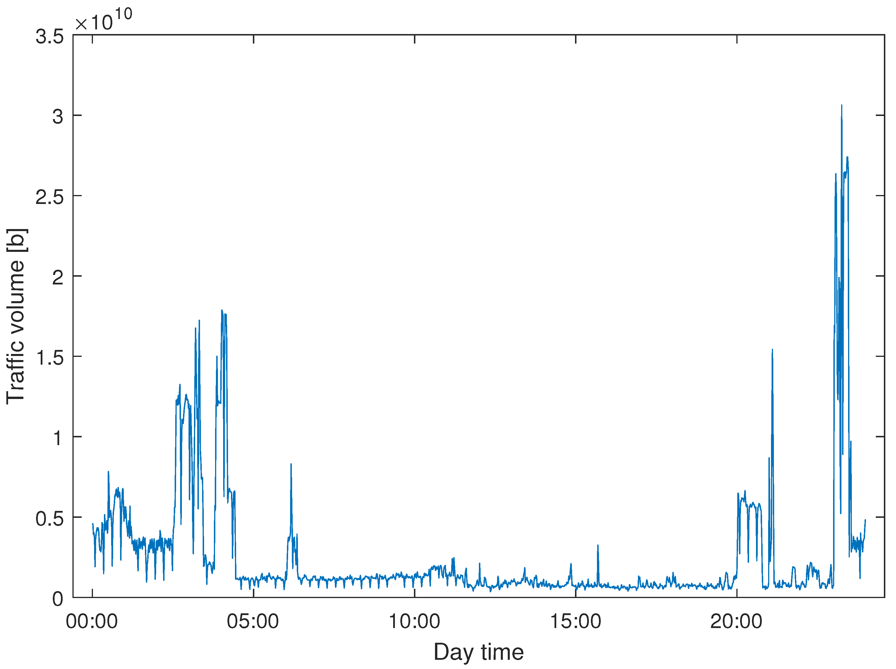
In this paper, we study the problem of efficient modeling and prediction of daily (i.e., long-term) traffic patterns in transport telecommunication networks. In our investigation, we use two historical traffic datasets from January 2021, namely, WASK and SIX. The datasets collect data from edge routers of two transport networks of different sizes, which affect the traffic characteristics and then the modeling/prediction process. It is worth mentioning that WASK is a novel dataset, which is introduced in this paper and has not been analyzed before. For the datasets, we propose long-term modeling and prediction approaches. For modeling, we use Fourier Transform analysis. For prediction, we propose and compare two methodologies: (i) modeling-based prediction (the forecasting model is assessed based on the historical traffic models) and (ii) machine learning-based (the network traffic is handled as a data stream where chunk-based regression methods are applied for prediction). We also perform extensive numerical experiments in order to verify efficiency of the proposed approaches and compare them. Since the datasets significantly differ in characteristics of the traffic, we also study how they influence the modeling and prediction performance.

The rest of the paper is organized as follows. Section 2 reviews the related works. Section 3 introduces the analyzed traffic datasets. Then, in Section 4, we describe the applied traffic modeling and prediction approaches. Section 5 presents the results of numerical experiments while Section 6 concludes the work.

2. Related Works

The consideration of historical traffic datasets in research and experiments is able to make the results more valuable and applicable in real networks. In turn, the data acquisition and publication are gaining more and more attention. The task is not trivial due to data privacy and security reasons. Therefore, the number of publicly available traffic datasets is deficient while their content is limited. One of the first publicly available datasets is SNDLIB library [15], which provides static and dynamic traffic matrices defined for several real network topologies. Unfortunately, the library is not being regularly updated and all the included data was gathered before 2014. Then, Seattle Exchange Point (SIX) [7] shares history of incoming/outgoing bit-rates (within a given time window) at routers located in the SIX. It is worth mentioning that SIX is currently one of the most popular traffic datasets in the research society, as it shares extensive and diverse statistics. It is especially widely applied for the task of traffic prediction in various configurations [11,12]. Similarly, several other platforms publish general information regarding observed traffic at Internet exchange points. However, the published information is usually only in the form of traffic plots, with no detailed numerical data available. For example, the AMS-ix [8] shares traffic plots from Amsterdam and collaborating locations and the ix.br [16] shares the graphical statistics from different locations in Brazil. We can also reach data regarding traffic from much smaller network points such as University Campus of AGH University of Science and Technology (Krakow, Poland) [17].

Due to the numerous limitations of available traffic datasets and the impossibility of their direct application in numerical experiments (lack of numerical data, information from only one network point), traffic modeling becomes increasing popular. The oldest and simultaneously most commonly used traffic model works under the assumption that traffic demands arrive to the network according to a Poisson process while their duration follows a negative exponential distribution [18,19,20]. These assumptions emerge from the traditional telephony networks and do not meet the transmission characteristics of nowadays telecommunication networks supporting a plethora of diversified services. Therefore, the researchers have made a number of attempts to propose more accurate models. For instance, the authors of [21] propose to use Pareto process for traffic modeling in wavelength division multiplexing (WDM) networks. Then, authors of. [22,23] study network-dedicated models built on the collected traffic flows within a specific time window. The authors of [24] suggest to model network traffic using mathematical functions such as piecewise linear function with mean value following the Gaussian distribution, sine function, and the combination of two first options. The paper contains only general model assumptions and does not provide a definition of the functions’ parameters. The modeling using trigonometric functions was also studied in [9,25]. Another interesting proposal was presented in [26,27], where the multivariable gravity model was introduced. It relates the bit-rate exchanged between a pair of nodes with real data related to the populations of the regions served by the network nodes, geographical distance between the nodes, and the economy level expressed by gross domestic product (GDP). It should be noted that each of the proposed models suffers from some limitations and, therefore, none of them was universally approved and applied in the research society.

Besides traffic modeling, the problem of traffic prediction has gained more and more popularity [4]. The existing literature mainly makes use of the autoregressive integrated moving average (ARIMA) method [28,29] and machine learning algorithms [30,31,32]. ARIMA is a statistical model that uses variations and data regressions to find patterns to model data or to predict future data. It was applied, for instance, in [28], where the authors used the traffic prediction module for the purpose of virtual topology reconfiguration. Similarly, the authors of [29] applied the provided prediction for the task of the virtual network topology adaptability. In terms of the machine learning-based forecasting, the majority of research makes use of various implementations of neural networks. For example, the authors of [32,33] used long short term memory (LSTM) method to predict the network traffic wherein The authors of [32] used the forecast to determine efficient resource reallocation in the optical data center networks. The authors of [30] applied the gated recurrent unit recurrent neural network (GRU RNN) enriched with a special evaluation automatic module (EAM), which has the task of automating the learning process and generalizing the prediction model with the best possible performance. The authors of [31] benefited from a nonlinear autoregressive neural network to design efficient resource allocation procedures for intra-data center networks. It is also worth-mentioning the paper [11], which compared three regressors (i.e., linear regression (LR), random forest (RF) and k-nearest neighbours (kNN)) used for the task of traffic forecasting. The presented literature reveals that the efficiency of a forecasting method strongly depends on the traffic dataset and there is no universal approach that performs best for all traffic flows.

The above-mentioned papers focus on short-term traffic prediction (i.e., the forecasting traffic volume for a next time stamp). To the best of the authors’ knowledge, long-term traffic prediction (i.e, traffic forecasting for a significantly longer period (several hours or a day)) in telecommunication networks has to yet to be addressed. Moreover, the research is generally deficient in studies covering long-term traffic prediction regardless of the traffic interpretation (network traffic, crowd traffic, cars traffic, etc). The only attempts to address the problem were presented in [34,35], where the authors apply neural networks to predict traffic of, respectively, cars in a highway and people in a Chinese city. Therefore, the presented paper fills the literature gaps by studying long-time traffic modeling and prediction in telecommunication networks.

3. Traffic Datasets

In this paper, we focus on two historical traffic datasets. The first one is novel and has not been studied in the literature so far. It is called WASK and refers to the flows observed at the edge routers of Wroclaw Academic Computer Network (Wroclaw, Poland). The second one is called SIX since it summarizes information regarding traffic volumes observed at Seattle Exchange Point (SIX) routers. The traffic observed in both points differs significantly in terms of its volume and characteristics (i.e., the shape as a time function and samples autocorrelation). The datasets used in the investigation are available online (https://www.kssk.pwr.edu.pl/goscien/trafficmodeling/ (accessed on 20 May 2021)).

3.1. WASK Dataset

WASK (polish: Wrocławska Akademicka Sieć Komputerowa) stands for Wrocław (in Poland) Academic Computer Network. The WASK network connects the academic institutions of Wrocław, providing them with access to Polish national network PIONIER and European network GÉANT2. Its infrastructure includes 23 nodes and over 120 km of fibre-optic routes. The nodes are located mainly in the buildings of Wrocław universities. The backbone of the network is based on the Alcatel-Lucent 7750 SR-7 switches as well as on Juniper MX switches (MX80, MX480, MX960). Both devices are equipped with 10 G interfaces. The edge router is Juniper M120 with Gigabit interfaces and 10 GE interface capability. This router is connected to NetIron XMR 16,000 edge switch of the PIONIER network by 10GE interface capability. It allows to connect the WASK network directly to the switches in Zielona Góra (Poland) and Opole (Poland) at the speed of 10 GB. In the years 2006–2008, additional nodes in Legnica, Polkowice, and Lubin were created as a part of the WASK network [36].

The WASK network connects over 500 local networks and over 15,000 computer stations. It is linked with the PIONIER network and with the European network GÉANT2. WASK also has interconnection points with such networks as TK TELEKOM, UPC, Dialog and direct connections with such operators as EXATEL, TK TELEKOM, TPSA. WASK is supervised and monitored by Wrocław Center for Networking and Supercomputing (abrr. WCSS) using OpenNMS platform, which allows to monitor the traffic on random routers, active WASK networks (routers, switches), and resources (network services servers and HPCs). For more details regarding WASK network, we refer to [36].

The WASK traffic data is prepared from the Flow (NetFlow) from a Firewall Device resources shared through the Open Science Resource Atlas (AZON) project. The project is made for sharing the resources of scientific units created in research, educational, and popularizing processes. Resources are integrated and adapted so that they can be easily searched and reused in science or business. For more details regarding the project, we refer to [37]. Resources contain anonymized output data of firewall devices, i.e., network traffic flows (connections established on the Internet) to and from the infrastructure of the Wrocław Centre for Networking and Supercomputing, collected from devices that protect the resources of this unit. The daily average of entries is around 320 million. An example resource can be obtained at [38].

3.1.1. Data Acquisition

At the end of each day, the output of the Nfdump [39] program is sent to the storage server. Data files were accessed directly from there. For the observed time of January 2021, there were 31 files with an overall size of about 3.126 TB. The processing of this data consists of mapping, reducing, and aggregation steps which are about to be described.

The output data produced by Nfdump is a 48-column csv file. The vast majority of those columns are, in the context of this research, irrelevant, so the first step was to strip those files to only three-columns files which contained the start, end, and size of each Netflow entry. Time marks are presented as standard timestamps while the size is a number of bytes which were transferred over the network during a given traffic flow. Then, the flows were processed in order to get the sampling rate of 1 min. At the end, the dataset consists of 44,640 aggregated flows, evenly distributed for each day. A total traffic volume for this dataset is about 173.88 TB for the whole time interval with a mean traffic slightly over 5.6 TB for each day.

The data acquisition, processing, and dataset generation were implemented with Python over the network through the ssh connection between the work station and the storage server, using the Dask Dataframe library [40] which allows for scalable analytics of larger-than-memory data. Such approach was necessary since the massive amount of data could not be computed using the standard approaches such as Pandas library [41] which is designed to always read the whole data into the memory.

3.1.2. Dataset Presentation

WASK dataset considered in this paper consists of traffic flows observed in January 2021. We have 31 days of observations wherein in each day the aggregated traffic volume was gathered every 1 min. Overall, the dataset consists of 31 days of 1440 observations what gives 44,640 data points in total.

Figure 1 presents the observed traffic volume on the 1st of January 2021. The traffic volume as a time function has a complicated and irregular process. It indicates that there are numerous components (i.e., network services) affecting and shaping the traffic. Nevertheless, we can notice a pattern there regarding intense traffic transmission at the night time (it starts at 20:00, then intensifies about 24:00, and decreases until 5:00). It is mainly determined by the data backups and inter-city synchronisations scheduled in the night-time, when typical end network users are less active. In order to check if the same patterns are also observed for other days, in Figure 2, we present the traffic volume observed during 31 days of January 2021 (each day is represented by a different colour) and in Figure 3, the dataset autocorrelation function. The first figure shows that traffic patterns observed within 31 subsequent days differ, wherein they have some common elements. For instance, the traffic intensification between 20:00 and 24:00 and the traffic decrease about 5:00 were observed in the majority of days. Moreover, many observations reveal intense traffic volume between 24:00 and 5:00. The autocorrelation function value for that set increases to approximately 0.4 after every 1440 lags, which indicates a moderate ccorrelations between data observed for subsequent days.

3.2. SIX Dataset

The SIX is an Internet Exchange Point in Seattle, Washington. They provide an interconnection between member networks in the Northwest United States and beyond. Networks connect at speeds from 1 to N × 100 Gbps. At the time of writing, SIX included 342 ASNs, 390 routers, and 344 members; 92 member-facing 100 GbE ports, 1 member-facing 40 GbE port, 277 member-facing, 10 GbE ports and 42 member-facing GigE ports. For more details regarding SIX, we refer to [7].

3.2.1. Data Acquisition

The SIX traffic data is available publicly on the Point’s website. The amounts of aggregated traffic are presented in the form of graphs. The raw values can be downloaded in a rrd format and later analysed using RRDTool. There are two sampling rates available, namely, 5 min and 1 min. We collected the 5 min sampling rrd files weekly, since that is the capacity of the published databases. That way, data with the same granularity is available for the whole investigated period.

3.2.2. Dataset Presentation

SIX dataset considered in this paper consists of traffic flows observed in January 2021. We have 31 days of observations wherein each day, the aggregated traffic volume was gathered every 5 min. Overall, the dataset consists of 31 days of 288 observation, which gives 8928 data points in total.

Figure 4 presents the observed traffic volume on the 1 January 2021. Compared to the WASK, the traffic time process has a significantly more regular and simple shape. It might suggest that due to the high data aggregation, there are fewer traffic components (i.e., services), which affect the traffic process in a noticeable way. The average SIX traffic volume is about two ranges of magnitude higher than that of WASK. The presented data reveals a flow intensification at SIX during the daytime (the traffic begins to increase about 20:00 and reaches its highest volume about 10:00–15:00). To verify whether there are common traffic patterns observed every day at SIX, we present Figure 5 with the traffic volume observed during 31 days of January 2021 (each day is represented by a different colour) and Figure 6 with the dataset autocorrelation function. According to Figure 5, almost the same traffic pattern is observed every day at SIX wherein the traffic volume (i.e., signal amplitude) changes. The existence of a common traffic pattern is also proved by the autocorrelation function (see Figure 6), which has a very regular shape and takes the highest values (initially above 0.9) every 288 lags, corresponding to consecutive days. That implies high daily seasonality.

4. Traffic Modeling and Prediction Methods

In this section, we present methods used for the purpose of traffic modeling and prediction. We also discuss their configuration and main application assumptions.

4.1. Traffic Modeling

Based on the analysis of WASK and SIX datasets (see Section 3), we assume that the traffic volume as a time function can be modeled using a trigonometric cosine signal according to Equation (1). The signal is a sum of a constant component $a_0$, N cosine functions (i.e., harmonics) $a_n·cos({\omega }_n·t+{\varphi }_n)$ and a noise $\sigma$.

$$f\left(t\right)=a_0+\sum _{n\in N}{a}_n·cos({\omega }_n·t+{\varphi }_n)+\sigma$$

(1)

where:

• $a_0$ constant component.
• $\sigma$ noise component.
• $a_n·cos({\omega }_n·t+{\varphi }_n)$n-th harmonic with amplitude $a_n$, pulsation ${\omega }_n$ and initial phase ${\varphi }_n$.

In order to determine signal’s harmonics, we perform its spectral analysis using Fourier Transform [42,43]. That mathematical transformation allows us to determine the constant component and signal harmonics with all their characteristics (i.e., amplitude, pulsation, and initial phase). To eliminate a noise signal from the signal modeling (i.e., to not model it as a signal harmonic), we take into account only harmonics with amplitude and phase higher than $ϵ={10}^{-6}$.

Based on the initial experiments, we assume that each day is a one-signal period and, therefore, we build a traffic model separately for each observation day. That assumption allows to achieve significantly higher modeling accuracy compared to the situation when one model is created for a period of several days.

The traffic modeling was implemented and evaluated using Matlab R2021a environment and build-in functions.

4.2. Traffic Prediction

For the purpose of traffic prediction, we propose and analyze two approaches—modeling-based and machine learning-based. For both approaches, we take into account a long-term traffic prediction where the size of a prediction window varies from 6 up to 24 h (the whole next day).

4.2.1. Modeling-Based Traffic Prediction

In the modeling-based traffic prediction, we build a traffic model (using Fourier Transform) for each historical day of traffic observations and then use the models to forecast traffic for the next day. We propose two approaches for traffic forecasting based on historical models–previous days (PD) and previous same days (PSD). The PD assumes that similar traffic patterns are observed for each day of the week. The prediction model is calculated here as a an average from a number of already built traffic models. The method is evaluated in two versions: (i) PD (1)—only one directly previous day (model) is taken into account, (ii) PD (all)—all previous days (models) are considered. Then, in the PSD, we assume that there are some separate traffic patterns observed for each day of the week (i.e., Monday, Tuesday, etc). The prediction model is defined here as an average from a number of already built traffic models for the same days of the week. Two method’s versions are studied: (i) PSD (1)—only one directly previous same week day (model) is taken into account, (ii) PSD (all)—all previous same week days (models) are taken into the consideration. T

Since we build a particular traffic model for a period of one day (24 h), the size of a prediction window in modeling-based approach is always 24 h.

4.2.2. Machine Learning-Based Traffic Prediction

Network traffic is an example of a data stream. That means it is a setting, where data comes to the system continuously and the dataset is constantly growing. Because of its potentially infinite volume, it is not possible to store and analyse the entire data stream in a real-life scenario, due to time and memory restrictions. For that reason, data streams are often divided into small portions called data chunks. That allows us to continuously update the model with new observations, so that it adjusts to the current conditions without the need for retraining. Such online methods are suitable to predict a series of values for different time horizons [44].

In this section, we compare instances of two main approaches used for chunk-based learning in data streams: an effective single estimator and an ensemble of estimators [45]. Because of a rather complex nature of WASK dataset, after initial testing of a number of classical machine learning algorithms, we propose a neural network-based approach. As the base estimator, we use the scikit-learn [46] implementation of the Multilayer Perceptron Regressor (MLP). For a direct comparison, we use it both stand-alone and as a base estimator for the Accuracy Weighted Ensemble (AWE) [47]. In the latter method, each estimator entering the pool is trained the same way but around a different data block and the forecast is a result of a weighted voting by the estimators present in the ensemble. With every iteration, a new estimator trained around the newest data chunk is added to the ensemble and the worst-performing one is deleted, so the size of the ensemble is constant.

As can be seen from the figures presented in Section 3, there is seasonality in the data. That means similar traffic patterns can be observed every day in considered datasets. Therefore, we use temporal additional features to improve the prediction quality, as proved to be useful in [11]. As in this work we consider a long-term forecast, we cannot use the most correlated previous timestamps as features. For that reason, we use the amount of traffic 24 h before the predicted datapoint as the first additional feature. As the second feature, we use a number indicating the day of the week, to take into account the weekly seasonality.

Machine learning-based traffic prediction was implemented in Python, using Scikit-learn, Pandas, SciPy and NumPy. After initial testing, we decided to change some of the default parameters of the MLP regressor to improve the prediction quality and time. The values of these parameters chosen after tuning are presented in

Table 1. Tuning the parameters for the MLP regressor.

Parameter	Chosen Value
‘hidden_layer_sizes’	(4,)
‘activation’	‘identity’
‘max_iter’	1000
‘warm_start’	True

. The remaining parameters were left with their default values.

For AWE, our own implementation was used. We applied the above-mentioned MLP regressor as the base estimator with the ensemble size set to 10. As shown in [48], quality metrics can be used as weighting methods in chunk-based learning in data streams, including AWE. For that reason, we used weighted voting proportional to the mean squared error. We applied the test-then-train evaluation [49], which means that every data chunk is used first for testing and then for training, and the model is updated incrementally after each data chunk.

5. Results and Discussion

In this section, we evaluate efficiency of the proposed traffic modeling and prediction approaches applied to WASK and SIX datasets.

5.1. Research Methodology

Before presenting the results of numerical experiments, let us briefly summarize and discuss the general research methodology including data acquisition and processing (if necessary) as well as the efficiency evaluation.

In all studies, the results accuracy is measured using mean absolute percentage error (MAPE) metric. For the sake of simplicity, we refer to this metric as error in the rest of the paper. Having an M-elements vector of historical data y and a vector of corresponding values obtained via modeling/prediction $y^{\prime }$, MAPE metric is calculated according to Equation (2).

$$MAPE=\frac{1}{M}·\sum _{m\in M}\frac{|y\left(m\right)-y^{\prime }\left(m\right)|}{y\left(m\right)}$$

(2)

Traffic Modeling

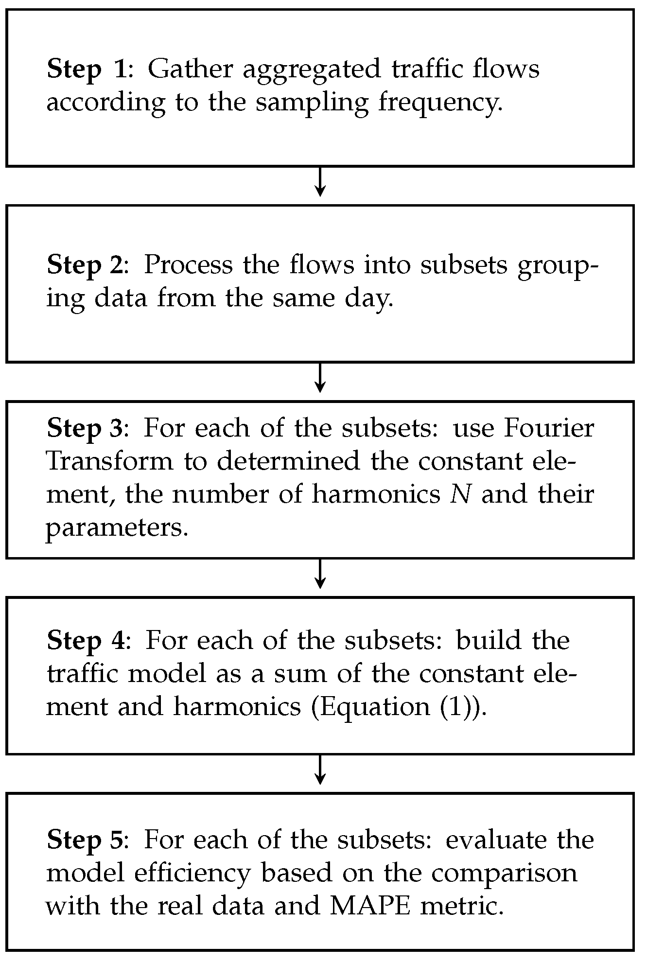
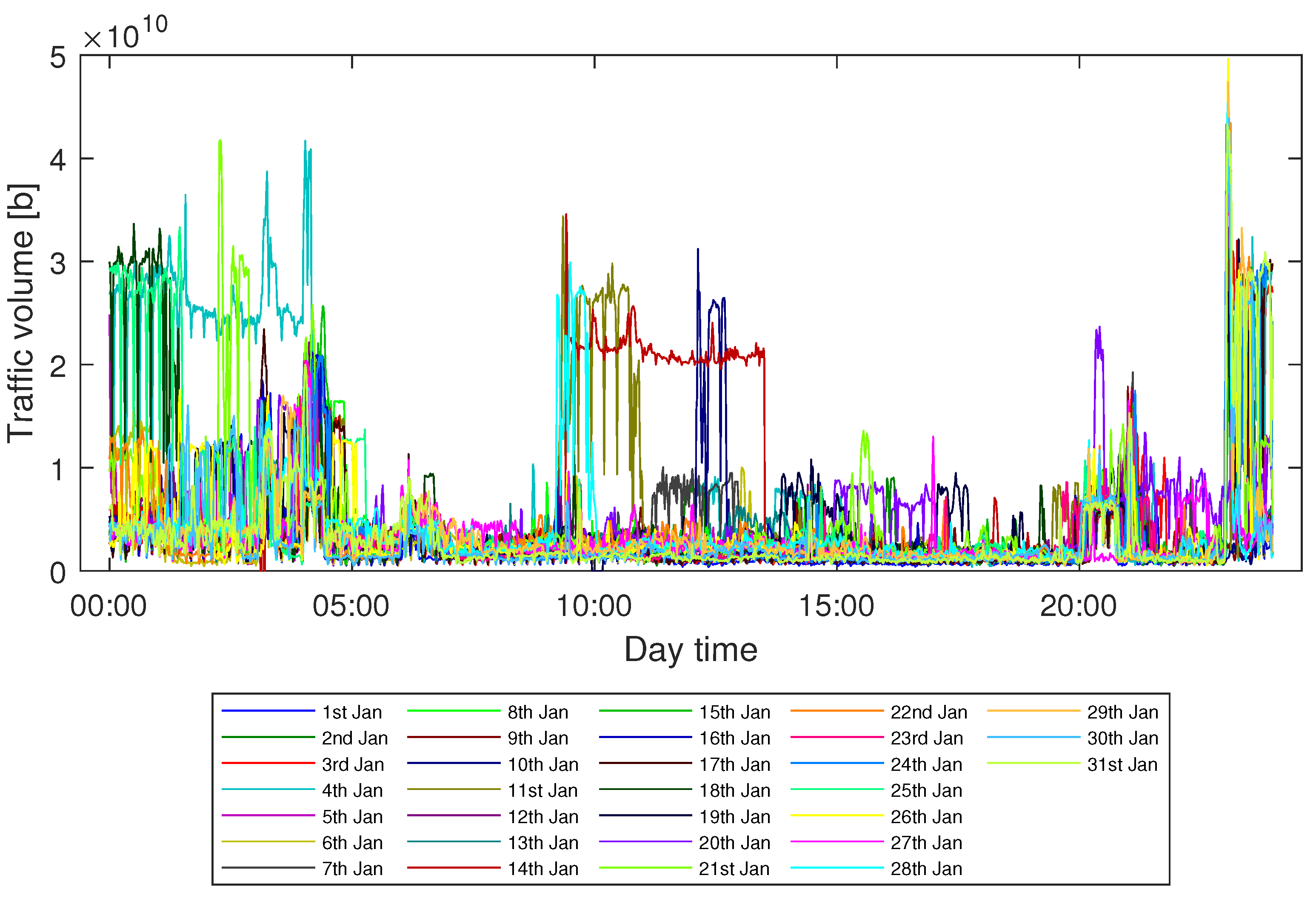
The idea of the traffic modeling and its efficiency evaluation is presented in Figure 7. At the beginning, it is necessary to create a traffic dataset by gathering traffic flows according to the sampling frequency (i.e., every 1 min for WASK and every 5 min for SIX). Then, the data has to be divided into the subsets grouping flows observed during the same day. In our study, the flows were gathered during January 2021 and 31 subsets were obtained for each dataset. In the next step, out modeling procedure is applied (see Section 4.1) to create a traffic model for each of the subsets (i.e., a separate traffic model is built for each day). The model efficiency is evaluated separately for each day by calculating average error value according to the MAPE metric. Please note that the results are averaged over 31 days and a number of observations during a single day (1440 for WASK and 288 for SIX).

5.2. Modeling-Based Traffic Prediction

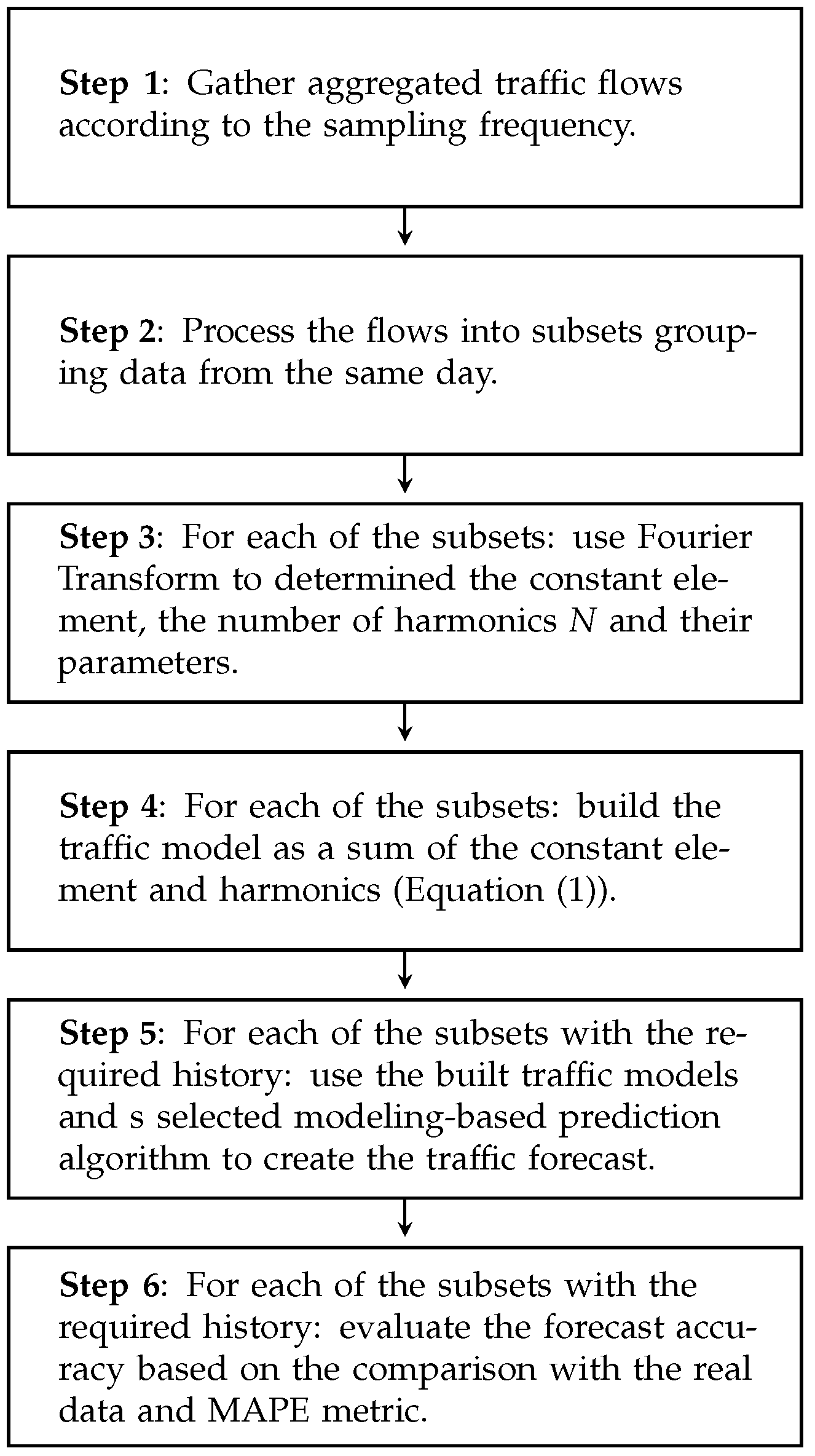
Then, the methodology of the modeling-based traffic prediction is presented in Figure 8. Since the approach benefits from the traffic modeling, it requires the same first steps as the traffic modeling (i.e., data acquisition, creation of one-day subsets, models creation for each of the days). Next, the approach moves to the creation of the forecasting model based on the selected already built traffic models (the number of including models depends on the selected forecasting algorithm and is described in detail in the next subsections). Please note that a forecasting model can be built only for a day with a history. Then, the accuracy of the forecasting models is evaluated separately for each day by calculating average error value according to the MAPE metric. Please not that the results are averaged over a number of days (with a history) and a number of observations during a single day (1440 for WASK and 288 for SIX).

Machine Learning-Based Traffic Prediction

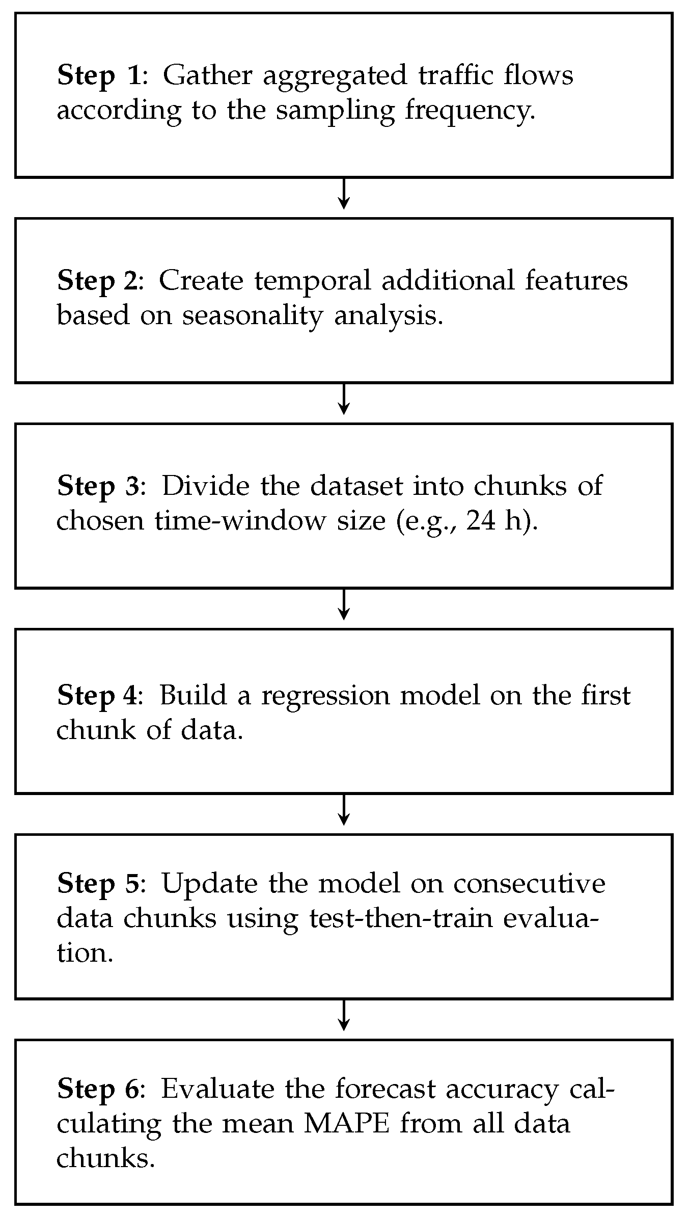
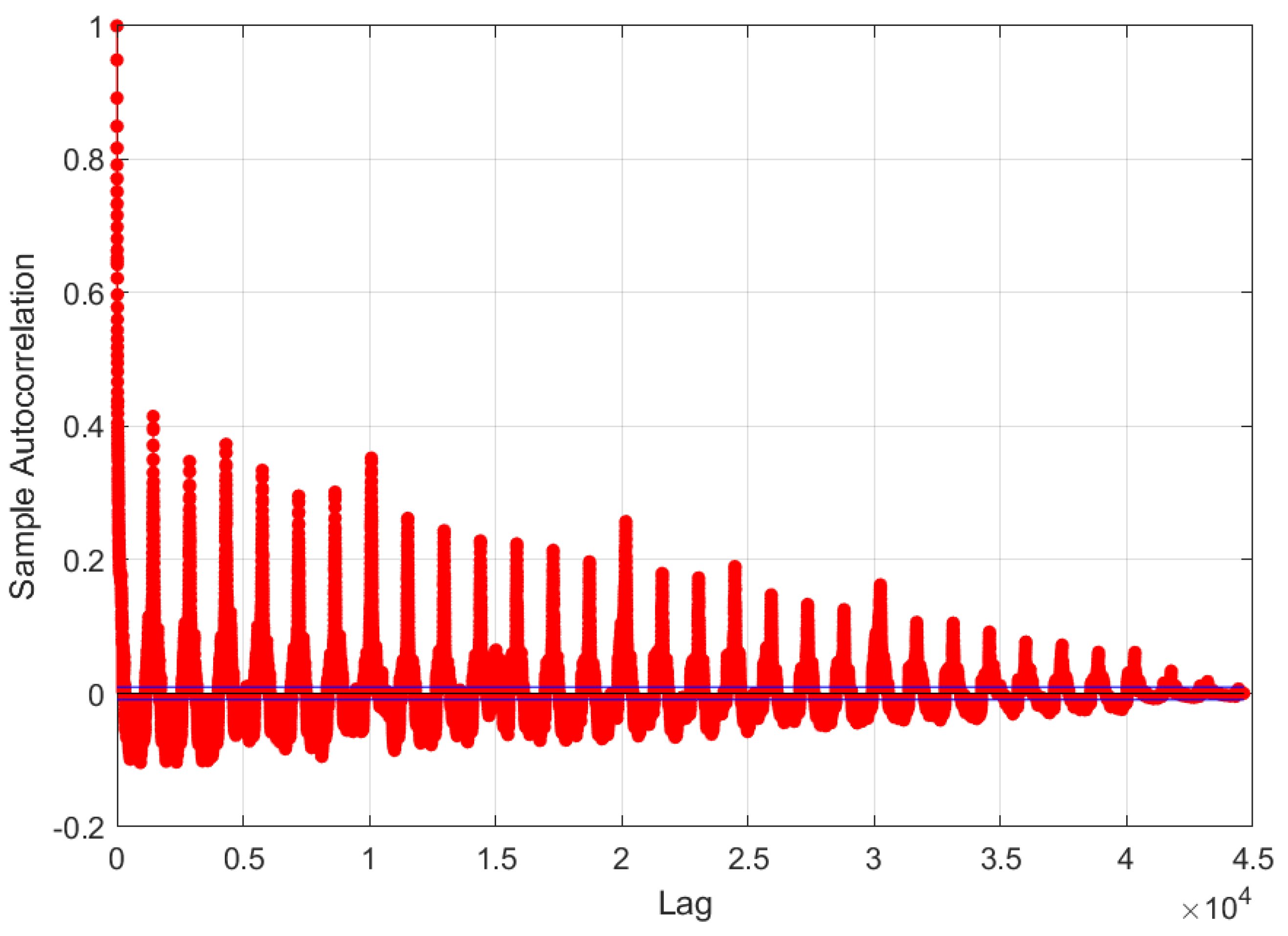
Finally, the methodology of the machine learning-based traffic prediction is presented in Figure 9. Similarly to traffic modeling and modeling-based prediction, the first step is to create a traffic dataset. In machine-learning based approaches, additional features are needed to make a forecast. In this work, they are created based on the seasonality analysis of considered datasets (see Section 3) and contain the amounts of traffic in past significant points in time. We use a chunk-based data stream approach, and for that reason, in the third step, the dataset is divided into smaller chunks. In the next step, a regression model is built around the first data chunk. On every consecutive data chunk, the model is continuously updated using test-then-train methodology. That means the model outputs a prediction for all samples in the chunk, which is then compared to real traffic values and the model is updated according to calculated MAPE value. To evaluate the overall forecast accuracy, the mean MAPE metric value is calculated from all the data chunks.

5.3. Traffic Modeling

First, we focus on the performance of the traffic modeling. For each dataset, we build a traffic model separately for each day of the month. Thus, the evaluation is prepared based on the evaluation of 31 models.

Table 2. Traffic modeling efficiency for WASK and SIX datasets.

	WASK	SIX
min error	0.0012	0.0000032033
avg error	0.0631	0.0009654600
max error	0.8605	0.0018000000
25th percentile error	0.0243	0.0007621800
50th percentile error	0.0310	0.0009330600
75th percentile error	0.0372	0.0012000000
standard deviation	0.1542	0.0003916600
avg processing time	0.0181 s	0.0030 s

reports the efficiency for two considered datasets. Since the results vary between different days of the month, we present a detailed analysis of the obtained errors and the corresponding standard deviation. Firstly, we observe that the quality of results obtained for two datasets differs much and is significantly higher for the SIX (the errors for SIX are smaller than these observed for WASK up to almost several orders of magnitude). For the WASK dataset, the average obtained error was 6.31%. However, the modeling efficiency significantly varies for different observation days. In turn, the minimum error was 0.12% while the highest was equal to 86.05%. It is worth mentioning than there were only two days of observation for which the modeling error was higher than 5%. The noticeable differences between modeling performance for various days are also confirmed by the high value of the standard deviation. Concurrently, the modeling accuracy for the SIX dataset is stable and outstanding—the maximum obtained error was equal to 0.16% while the average error was less than 0.1%. Moreover, the results were stable and characterized by a low standard deviation.

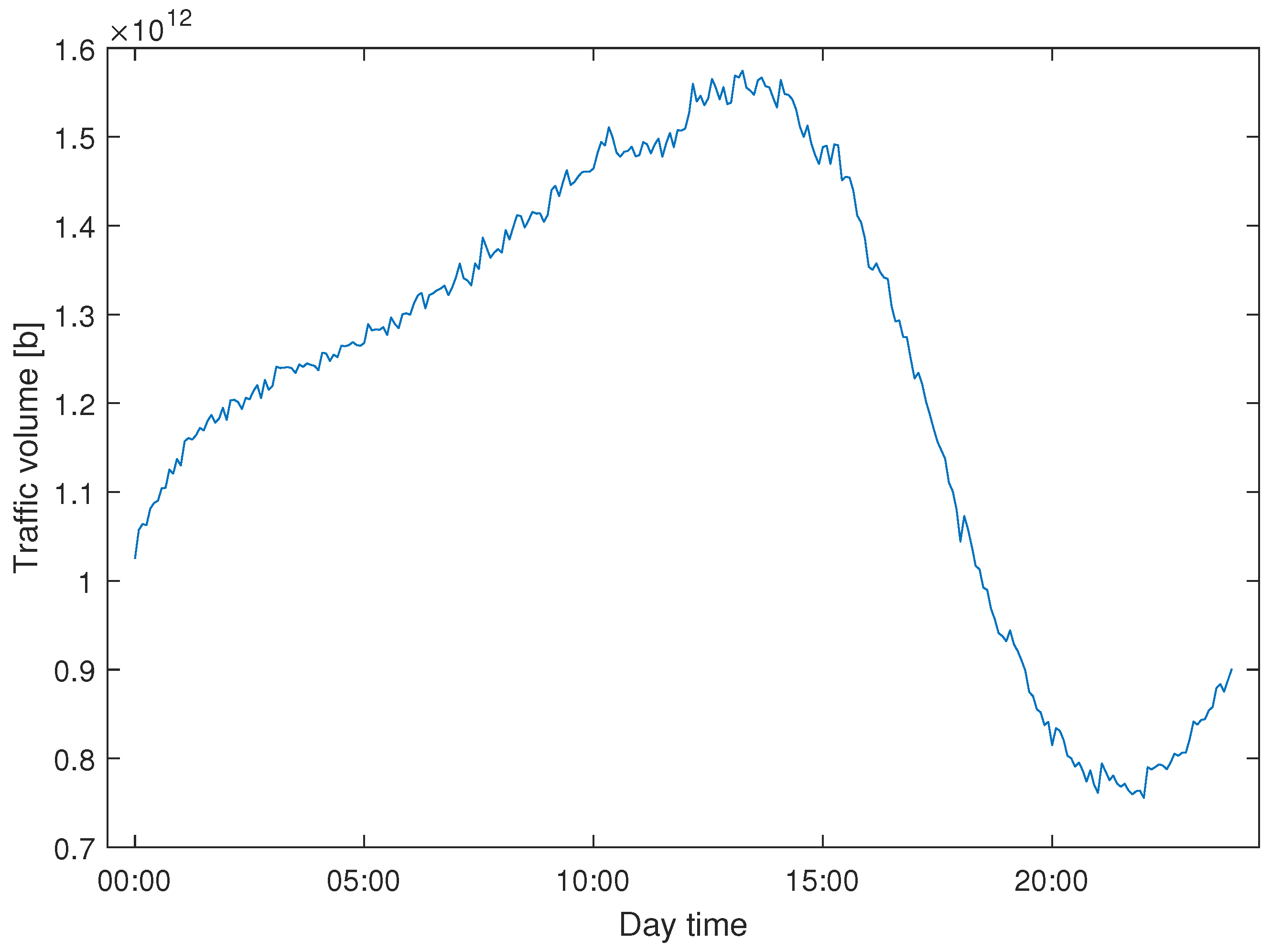
The outstandingly high modeling accuracy observed for SIX dataset proves that the applied sampling frequency (i.e., flows gathered every 5 min) for that traffic was properly selected. Since the modeling precision for WASK dataset was about two ranges of magnitude smaller, we can conclude that the sampling frequency (i.e., flows gathered over 1 min) applied for that traffic was not high enough to accurately project the signal process and variability. Therefore, the modeling accuracy for WASK might be improved by applying a higher sampling frequency.

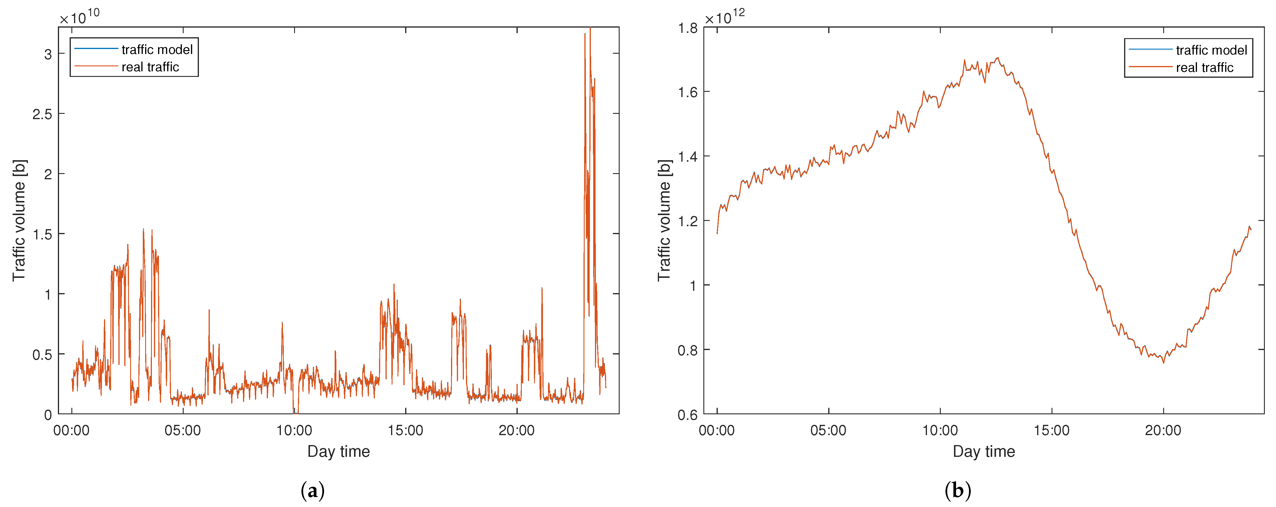
Figure 10 vizualizes the modeling performance for WASK and SIX datasets. The results are presented for two selected days for which the modeling approach performed the worst (i.e., maximum error obtained). Despite the high error values, the modeled signal properly follows the pattern of real data and the differences between the signal are hardly visible to the naked eye.

It is also worth mentioning that the number of significant harmonics for WASK was 1440 while for the SIX was 720 for each of the considered days. That proves our initial assumptions regarding time shapes of both traffics. WASK flow is determined by significantly more components (i.e., services) than SIX flow due to the different level of users/data aggregation.

Please note that the number of the harmonics influences also the modeling processing time (see Table 2), which is about six times higher for WASK dataset. Nevertheless, the calculation of a traffic model is a fast process and takes less than a second.

5.4. Traffic Prediction

The efficiency evaluation of traffic prediction is performed separately for modeling-based and machine learning-based approach.

5.5. Modeling-Based Traffic Prediction

In the context of modeling-based traffic prediction, the period for which the modeling is applied (i.e., 24 h) determines the size of a prediction window. The forecasting efficiency is summarized in

Table 3. Efficiency of modeling-based traffic prediction for WASK dataset.

	PD (1)	PD (All)	PSD (1)	PSD (All)
min error	32.0721	0.3469	0.3550	0.3604
avg error	139.0686	4.4537	4.1392	3.9610
max error	2007.7000	83.3229	45.5051	42.0399
25th percentile error	37.4813	0.4845	0.4627	0.5007
50th percentile error	43.7405	0.6688	0.6154	0.6113
75th percentile error	51.4728	0.7857	1.0215	1.0046
standard deviation	390.0556	16.0119	11.6286	11.1107
average processing time	0.0183 s	0.2801 s	0.0183 s	0.0455 s

and

Table 4. Efficiency of modeling-based traffic prediction for SIX dataset.

	PD (1)	PD (All)	PSD (1)	PSD (All)
min error	0.0175	0.0165	0.0157	0.0169
avg error	0.0416	0.0416	0.0322	0.0336
max error	0.0853	0.0695	0.0950	0.0950
25th percentile error	0.0294	0.0345	0.0218	0.0229
50th percentile error	0.0384	0.0383	0.0268	0.0280
75th percentile error	0.0515	0.0515	0.0385	0.0399
standard deviation	0.0166	0.0121	0.0167	0.0167
average processing time	0.0031 s	0.0466 s	0.0031 s	0.0076 s

, accordingly, for WASK and SIX datasets. The analysis comes from 30 days of observations (starting from 02.01.2021) and corresponding predictions. For both datasets the best results were obtained by PSD (all) method. It proves the hypothesis that different traffic patterns are observed for different days of the week. The prediction errors for SIX dataset reached up to almost 10% while keeping its average value on the level about 3–4%. The errors yielded for WASK dataset are much larger (even several orders of magnitude) and characterized by high standard deviation. Therefore, the investigation shows that modeling-based traffic prediction is suitable only for an easy dataset (such as SIX) and does not tackle well with complex data (such as, for instance, WASK traffic). Please note the accuracy of modeling-based traffic prediction is strongly determined by the precision of the built traffic models (see Table 2), which were outstanding for SIX and significantly weaker for WASK dataset.

The processing time of the modeling-based prediction includes the time required to build the history models and the time required to build a forecasting model. Therefore, it is mostly determined by the number of historical models, which are required. In turn, it is the shortest for PSD (1)/PD (1) and the longest for PD (all). We also observe that the calculations take slightly longer for the SIX dataset; however, they are fast and smaller than a second.

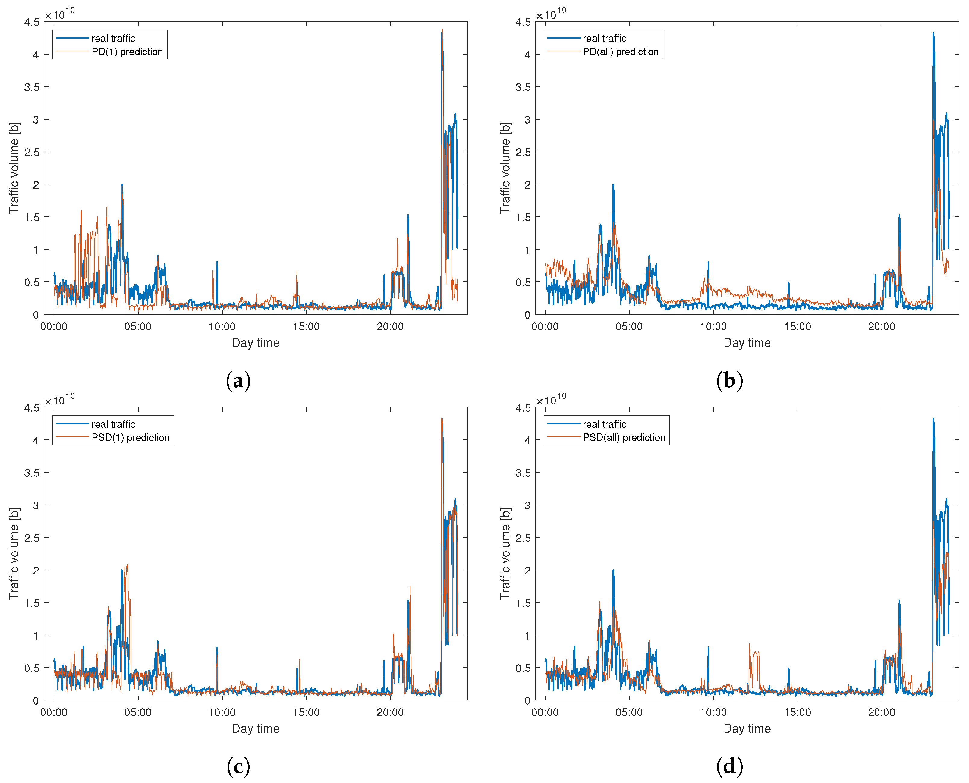
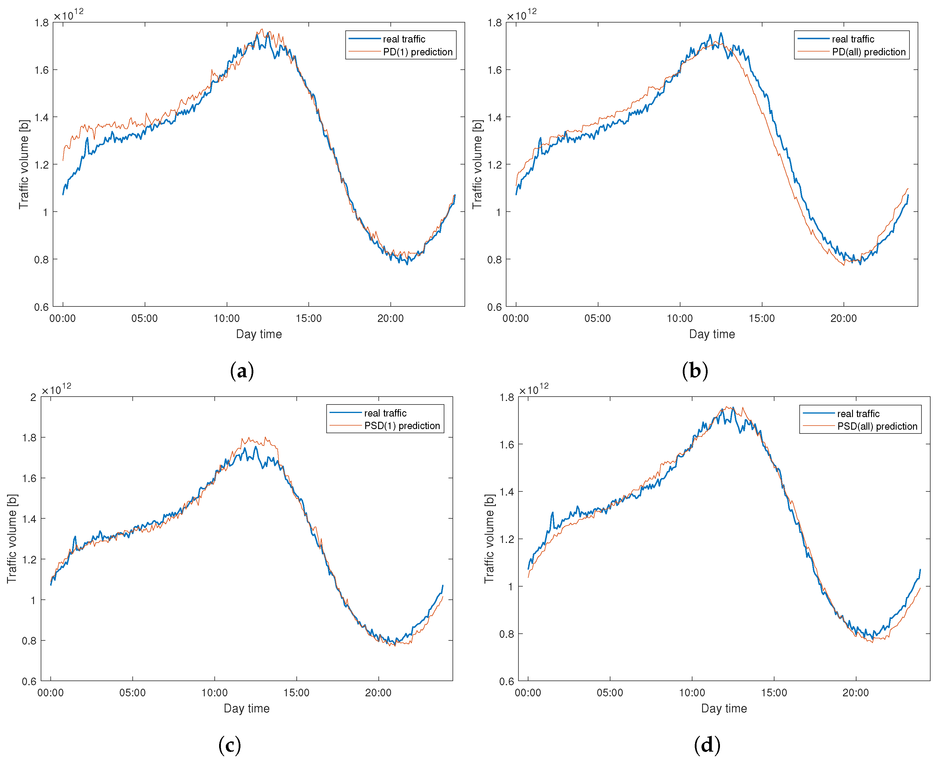
To better visualize method performance, Figure 11 presents a comparison of the predicted and real traffic for WASK on 31.01.2021. Similarly, Figure 12 reports the same dependence for SIX dataset. In both cases, we can clearly notice the differences between the real and predicted signal. They are especially significant for WASK dataset, where the trajectories of two signals differ. For the SIX dataset, the predicted signal correctly follows the real signal trajectory while the errors emerge from the amplitude over/under estimation.

5.6. Machine Learning-Based Traffic Prediction

In this section, we compare the prediction quality of two machine learning (chunk-based data stream) traffic forecasting methods (MLP and AWE) for three chosen time windows. The algorithms output a prediction for the next chunk of data, which is a series of datapoints. The series is then compared with a series of real values of the chunk and an error is calculated. Note that the granularity of gathered samples varies between considered datasets, so the number of points for the same time window is different for WASK and SIX.

Table 5. Efficiency of machine learning-based traffic prediction for WASK dataset for different time windows.

	24 h		12 h		6 h
	MLP	AWE	MLP	AWE	MLP	AWE
min error	0.3294	0.2843	0.2702	0.2278	0.1895	0.1906
avg error	0.8247	0.9685	0.8216	0.9580	0.8285	0.9040
max error	5.0686	6.7665	9.9583	12.5490	20.5203	24.1079
25th percentile error	0.4492	0.4761	0.4168	0.4080	0.3540	0.3487
50th percentile error	0.6049	0.6121	0.4880	0.5573	0.4586	0.4726
75th percentile error	0.6969	0.7808	0.6956	0.8048	0.6373	0.6745
standard deviation	0.9206	1.2536	1.3562	1.7575	2.0053	2.3657
avg processing time	0.0011 s	0.0104 s	0.0011 s	0.0118 s	0.0012 s	0.0120 s

presents the results of machine learning-based prediction for the WASK dataset. As can be seen, the MLP method achieved lower average error values for all the considered time windows. Furthermore, the results of MLP were more stable among data chunks, as proven by lower values of standard deviation. Comparing the results for different time windows, it can be noted that despite a rather stable average error within each method, the smaller the time window, the higher the value of standard deviation. That means smaller data chunks were generally more precisely predicted. That is visible when analysing the values of minimum error and the 25th and 50th percentiles—they decrease with the decrease in the time window. However, some of the data chunks were extraordinarily difficult to forecast, hence the high values of the maximum error, rising with the decrease in the time window size. It can be concluded that having chosen a smaller time window, one can expect a generally precise forecast, risking rare but high mistakes.

Table 6. Efficiency of machine learning-based traffic prediction for SIX dataset for different time windows.

	24 h		12 h		6 h
	MLP	AWE	MLP	AWE	MLP	AWE
min error	0.0183	0.0246	0.0122	0.0152	0.0002	0.0067
avg error	0.0443	0.0617	0.0571	0.0643	0.0421	0.0449
max error	0.0857	0.0976	0.1570	0.1674	0.1271	0.1331
25th percentile error	0.0333	0.0445	0.0345	0.0406	0.0214	0.0201
50th percentile error	0.0417	0.0659	0.0525	0.0564	0.0317	0.0340
75th percentile error	0.0564	0.0789	0.0728	0.0827	0.0542	0.0579
standard deviation	0.0167	0.0205	0.0298	0.0312	0.0284	0.0301
avg processing time	0.0012 s	0.0099 s	0.0013 s	0.0122s	0.0012 s	0.0109 s

presents the results of machine learning-based prediction for the SIX dataset. Comparing to the WASK dataset, the results are outstanding, with the average error being an order of magnitude lower. Similarly to the previously analyzed dataset, MLP achieved lower error values than AWE. Contrary to WASK, there is no clear trend visible in the prediction for different time windows. The lowest average error was obtained for the 6 h window in both methods, with the lowest standard deviation obtained for the 24 h window. However, the standard deviation values for all the time windows are much lower for the SIX dataset when compared to the WASK dataset. That means the prediction error is stable for consecutive data chunks.

Note that machine learning-based prediction outperforms modeling-based prediction for WASK dataset (see Table 3 vs. Table 5) regardless of the applied forecasting method (i.e., MLP or AWE). On the contrary, for the SIX dataset, the modeling-based prediction achieves higher efficiency (Table 4 vs. Table 6). The results show that none of the prediction approaches is principally better. To obtain high predictions accuracy, the forecasting method should be properly suited to the considered dataset.

The processing time of MLP-based forecasting oscillates around 0.01 seconds while the time of AWE-based forecasting is around 0.1 s (see Table 5 and Table 6). It does not vary much between two datasets and different window sizes. Comparing it with the times of the best modeling-based prediction methods (i.e., PSD (1), PSD (all), see Table 3 and Table 4), we observe that for WASK, the machine learning-based prediction works faster; however, both methodologies provide fast calculations. In the cast of SIX, MLP runs the fastest, then the modeling-based method, and finally AWE.

Taking into account the prediction accuracy and time of calculations, for the long-term traffic prediction, we recommend the use of a modeling-based approach for SIX (i.e., for more stable and regular traffic) and machine-learning for WASK (i.e., for irregular traffic with a high variability).

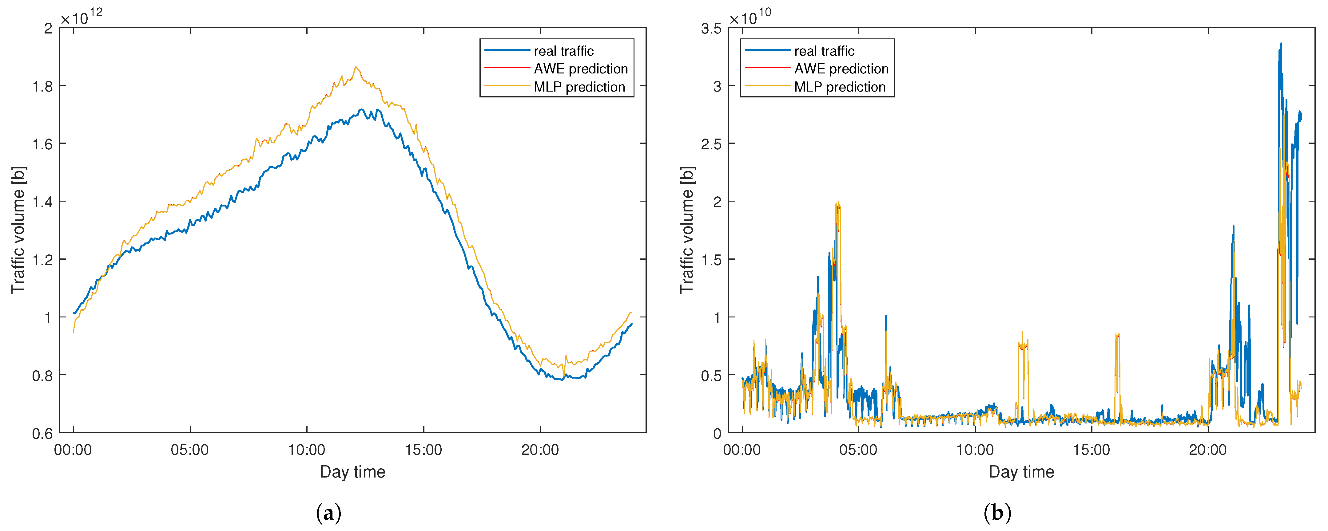
Figure 13 presents the prediction results for the first predicted day in both datasets (2 January 2021) for the 24 h time window. The machine learning models were only trained with one day worth of data at that point. As can be seen, they are able to follow the general pattern and predict the traffic with no substantial mistakes. This proves that the proposed methods do not require previous offline training on large volumes of data, they are ready to use after only one day, even for a difficult dataset like WASK. Interestingly, the predictions made by both models are almost identical in the first day in both datasets. That is due to the fact that in the first predicted chunk of data, the ensemble size in AWE is 1—there is only one estimator trained on the previous portion of data. Since the base estimator for AWE is the MLP regressor itself, the predictions made by both models match almost perfectly and the differences between them are not visible to the naked eye at this point.

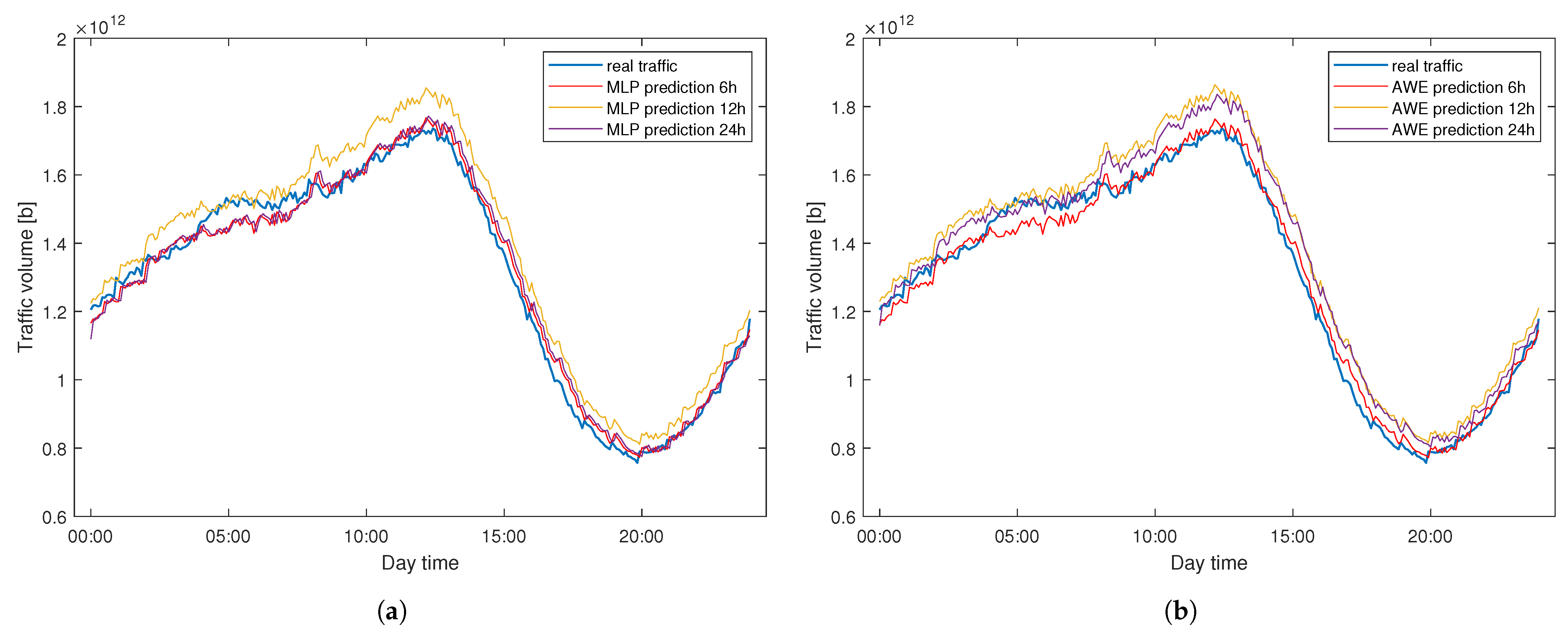
Figure 14 presents the predictions made by the same methods but with different time windows in a sample day for the SIX dataset. That means that for the 24 h time window, the one-day forecast is composed of one chunk of data, for the 12 h, two chunks, and four chunks for the 6 h window. Separate lines can be spotted by the naked eye, revealing slight differences in prediction efficiency. Figure 15 presents the predictions made by the same methods with different time windows in a sample day for the WASK dataset. Similarly to SIX, slight differences are visible.

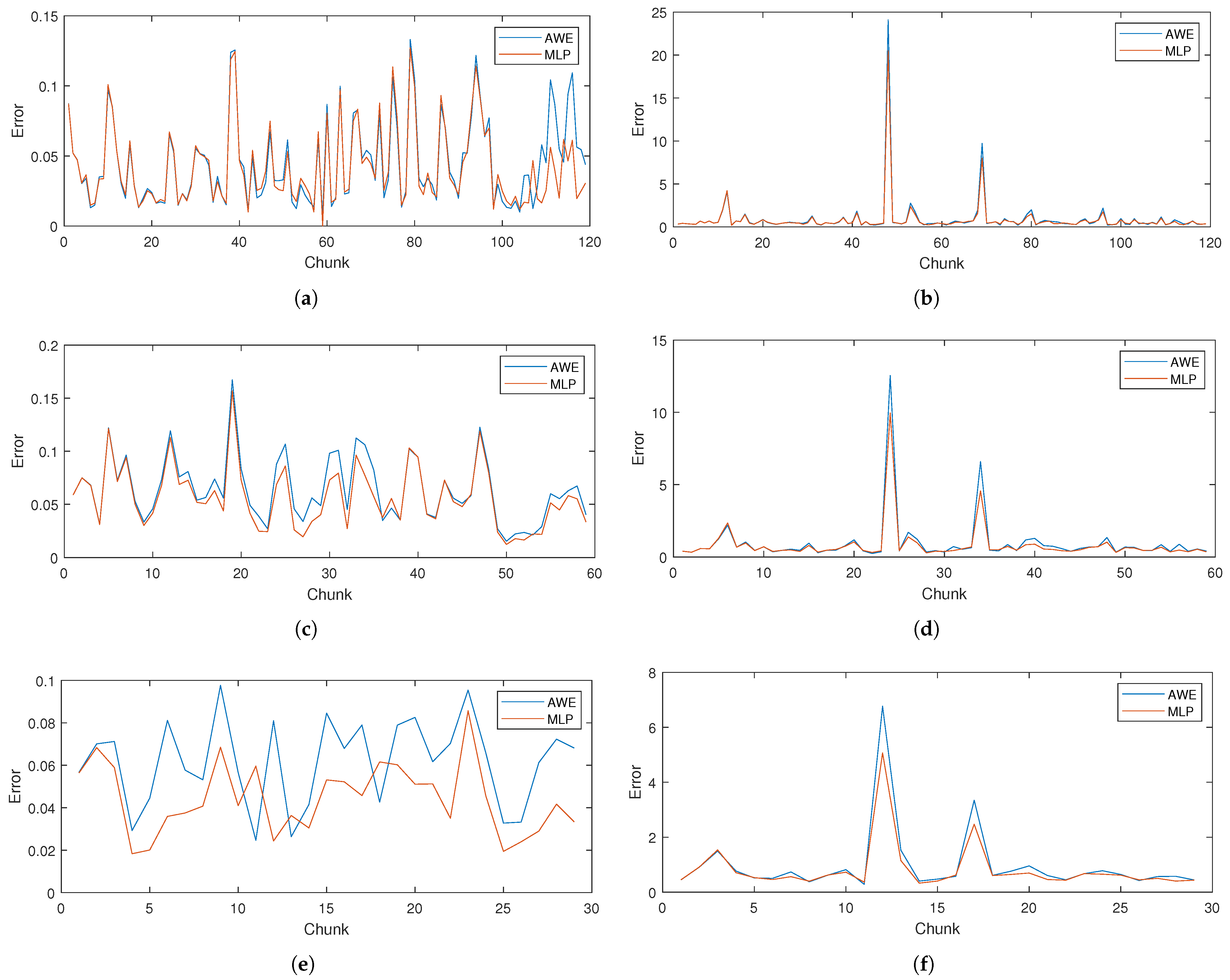
Finally, Figure 16 presents the error values for consecutive chunks of data for different time windows in both methods for considered datasets. As can be seen, the proposed models are able to react to changes in traffic volume and adapt to current conditions. Moreover, these figures illustrate the span of errors in both datasets. Datapoints exceptionally difficult to predict (with prediction errors much higher than average) are only present in the WASK dataset. The error peaks indicating difficult-to-predict moments in the network traffic time-series are followed by rapid troughs, as models adjust their predictions. The error values are on a stable level for the vast majority of data chunks and both methods follow the same error values patterns. On the other hand, in the SIX dataset, the differences in error patterns between considered methods are much easier to spot. However, their values are generally on a stable level, as pointed out discussing their standard deviations.

6. Conclusions

In this paper, we focused on the efficient modeling and prediction of the daily traffic patterns in the transport telecommunication networks. We used two historical datasets (WASK and SIX), which significantly differ with the characteristics. Since WASK is a completely new dataset, we introduced it and discussed in detail. Then, we proposed modeling and prediction methods. For the modeling, we applied Fourier Transform while for the forecasting we studied two approaches—modeling-based (i.e., PD (1), PD (all), PSD (1), PSD (all)) and machine learning-based (i.e., MLP and AWE).

We evaluated the efficiency of the proposed methods by means of extensive simulations. In the traffic modeling, we achieved the outstanding results of an average error of less than 0.1% in SIX and 6.31% in WASK. In the case of traffic prediction, the modeling-based approach was better for SIX while machine learning-based performed superior for WASK dataset. The average prediction error for SIX was 3.22% (for the best method) while the forecasting for WASK revealed a much more complex nature.

In future work, we are going to further explore WASK dataset by gathering more data and verifying existence of patterns between different months. We plan to use the datasets and proposed models to support network optimization.

References

1. Lukasik, S. Why the Arpanet Was Built. IEEE Ann. Hist. Comput. 2011, 33, 4–21. [Google Scholar] [CrossRef]
2. Lutu, A.; Perino, D.; Bagnulo, M.; Frias-Martinez, E.; Khangosstar, J. A Characterization of the COVID-19 Pandemic Impact on a Mobile Network Operator Traffic. In Proceedings of the ACM Internet Measurement Conference, Association for Computing Machinery, 2020; pp. 19–33. Available online: https://dl.acm.org/doi/abs/10.1145/3419394.3423655 (accessed on 20 May 2021).
3. Cisco Annual Internet Report 2018–2023 White Paper. 2020. Available online: https://www.cisco.com/c/en/us/solutions/collateral/executive-perspectives/annual-internet-report/white-paper-c11-741490.html (accessed on 20 May 2021).
4. Musumeci, F.; Rottondi, C.; Nag, A.; Macaluso, I.; Zibar, D.; Ruffini, M.; Tornatore, M. An Overview on Application of Machine Learning Techniques in Optical Networks. IEEE Commun. Surv. Tutor. 2019, 21, 1383–1408. [Google Scholar] [CrossRef] [Green Version]
5. Goścień, R.; Walkowiak, K.; Klinkowski, M. Distance-adaptive transmission in cloud-ready elastic optical networks. J. Opt. Commun. Netw. 2014, 6, 816–828. [Google Scholar] [CrossRef]
6. Xie, J.; Yu, F.R.; Huang, T.; Xie, R.; Liu, J.; Wang, C.; Liu, Y. A Survey of Machine Learning Techniques Applied to Software Defined Networking (SDN): Research Issues and Challenges. IEEE Commun. Surv. Tutor. 2019, 21, 393–430. [Google Scholar] [CrossRef]
7. Seattle Internet Exchange. Available online: https://www.seattleix.net/statistics/ (accessed on 20 May 2021).
8. Amsterdam Internet Exchange. Available online: https://stats.ams-ix.net/index.html (accessed on 20 May 2021).
9. Rzym, G.; Boryło, P.; Chołda, P. A time-efficient shrinkage algorithm for the Fourier-based prediction enabling proactive optimisation in software-defined networks. Int. J. Commun. Syst. 2020, 33, e4448. [Google Scholar] [CrossRef]
10. Zhong, Z.; Hua, N.; Yuan, Z.; Li, Y.; Zheng, X. Routing without Routing Algorithms: An AI-Based Routing Paradigm for Multi-Domain Optical Networks. In 2019 Optical Fiber Communications Conference and Exhibition (OFC); Optical Society of America: Washington, DC, USA, 2019. [Google Scholar]
11. Knapińska, A.; Lechowicz, P.; Walkowiak, K. Machine-Learning Based Prediction of Multiple Types of Network Traffic. In Lecture Notes in Computer Science, Proceedings of the International Conference on Computational Science–ICCS 2021, Krakow, Poland, 16–18 June 2021; Springer International Publishing: Berlin, Germany, 2021; Volume 12742, pp. 122–136. [Google Scholar]
12. Szostak, D.; Walkowiak, K.; Włodarczyk, A. Short-Term Traffic Forecasting in Optical Network using Linear Discriminant Analysis Machine Learning Classifier. In Proceedings of the 2020 22nd International Conference on Transparent Optical Networks (ICTON), Bari, Italy, 19–23 July 2020; pp. 1–4. [Google Scholar] [CrossRef]
13. Cenedese, A.; Tramarin, F.; Vitturi, S. An Energy Efficient Ethernet Strategy Based on Traffic Prediction and Shaping. IEEE Trans. Commun. 2017, 65, 270–282. [Google Scholar] [CrossRef]
14. Guan, L.; Zhang, M.; Wang, D. Demonstration of AI-Assisted Energy-Efficient Traffic Aggregation in 5G Optical Access Network. In 2020 Optical Fiber Communications Conference and Exhibition (OFC); Optical Society of America: Washington, DC, USA, 2020; pp. 1–3. [Google Scholar]
15. Orlowski, S.; Pióro, M.; Tomaszewski, A.; Wessäly, R. SNDlib 1.0—Survivable Network Design Library. In Proceedings of the 3rd International Network Optimization Conference (INOC 2007), Spa, Belgium, 12–14 June 2007. [Google Scholar]
16. Brazil Internet Exchange. Available online: https://ix.br/agregado/ (accessed on 20 May 2021).
17. Jurkiewicz, P.; Rzym, G.; Borylo, P. Flow length and size distributions in campus Internet traffic. Comput. Commun. 2021, 167, 15–30. [Google Scholar] [CrossRef]
18. Ba, S.; Chatterjee, B.C.; Oki, E. Defragmentation Scheme Based on Exchanging Primary and Backup Paths in 1+1 Path Protected Elastic Optical Networks. IEEE/ACM Trans. Netw. 2017, 25, 1717–1731. [Google Scholar] [CrossRef]
19. Goścień, R. On the efficient dynamic routing in spectrally-spatially flexible optical networks. In Proceedings of the Resilient Networks Design and Modeling (RNDM), Nicosia, Cyprus, 14–16 October 2019. [Google Scholar]
20. Walkowiak, K.; Klinkowski, M.; Lechowicz, P. Dynamic routing in spectrally spatially flexible optical networks with back-to-back regeneration. IEEE/OSA J. Opt. Commun. Netw. 2018, 10, 523–534. [Google Scholar] [CrossRef]
21. Gaizi, K.; Abdi, F.; Abbou, F.M. Realistic dynamic traffic generation for WDM Optical Networks. In Proceedings of the 2016 27th Irish Signals and Systems Conference (ISSC), Londonderry, UK, 21–22 June 2016; pp. 1–4. [Google Scholar] [CrossRef]
22. Gencata, A.; Mukherjee, B. Virtual-topology adaptation for WDM mesh networks under dynamic traffic. IEEE/ACM Trans. Netw. 2003, 11, 236–247. [Google Scholar] [CrossRef]
23. Troia, S.; Cibari, A.; Alvizu, R.; Maier, G. Dynamic programming of network slices in software-defined metro-core optical networks. Opt. Switch. Netw. 2020, 36, 100551. [Google Scholar] [CrossRef] [Green Version]
24. Vela, A.P.; Vía, A.; Morales, F.; Ruiz, M.; Velasco, L. Traffic generation for telecom cloud-based simulation. In Proceedings of the 2016 18th International Conference on Transparent Optical Networks (ICTON), Trento, Italy, 10–14 July 2016; pp. 1–4. [Google Scholar] [CrossRef]
25. Goścień, R. Traffic-Aware Service Relocation in Cloud-Oriented Elastic Optical Networks. 2021. Available online: http://xxx.lanl.gov/abs/2105.07653 (accessed on 20 May 2021).
26. Goścień, R.; Walkowiak, K.; Klinkowski, M.; Rak, J. Protection in elastic optical networks. IEEE Netw. 2015, 29, 88–96. [Google Scholar] [CrossRef]
27. Klinkowski, M.; Walkowiak, K. On the advantages of elastic optical networks for provisioning of cloud computing traffic. IEEE Netw. 2013, 27, 44–51. [Google Scholar] [CrossRef]
28. Fernández, N.; Barroso, R.J.D.; Siracusa, D.; Francescon, A.; de Miguel, I.; Salvadori, E.; Aguado, J.C.; Lorenzo, R.M. Virtual topology reconfiguration in optical networks by means of cognition: Evaluation and experimental validation [invited]. IEEE/OSA J. Opt. Commun. Netw. 2015, 7, A162–A173. [Google Scholar] [CrossRef]
29. Morales, F.; Ruiz, M.; Gifre, L.; Contreras, L.M.; Lopez, V.; Velasco, L. Virtual network topology adaptability based on data analytics for traffic prediction. IEEE/OSA J. Opt. Commun. Netw. 2017, 9, A35–A45. [Google Scholar] [CrossRef]
30. Troia, S.; Alvizu, R.; Zhou, Y.; Maier, G.; Pattavina, A. Deep Learning-Based Traffic Prediction for Network Optimization. In Proceedings of the 2018 20th International Conference on Transparent Optical Networks (ICTON), Bucharest, Romania, 1–5 July 2018; pp. 1–4. [Google Scholar] [CrossRef] [Green Version]
31. Balanici, M.; Pachnicke, S. Machine Learning-Based Traffic Prediction for Optical Switching Resource Allocation in Hybrid Intra-Data Center Networks. In 2019 Optical Fiber Communications Conference and Exhibition (OFC); Optical Society of America: Washington, DC, USA, 2019. [Google Scholar]
32. Singh, S.K.; Jukan, A. Machine-learning-based prediction for resource (Re)allocation in optical data center networks. IEEE/OSA J. Opt. Commun. Netw. 2018, 10, D12–D28. [Google Scholar] [CrossRef]
33. Lu, H.; Yang, F. Research on Network Traffic Prediction Based on Long Short-Term Memory Neural Network. In Proceedings of the 2018 IEEE 4th International Conference on Computer and Communications (ICCC), Chengdu, China, 7–10 December 2018; pp. 1109–1113. [Google Scholar]
34. Qu, L.; Li, W.; Li, W.; Ma, D.; Wang, Y. Daily long-term traffic flow forecasting based on a deep neural network. Expert Syst. Appl. 2019, 121, 304–312. [Google Scholar] [CrossRef]
35. He, Z.; Chow, C.Y.; Zhang, J.D. STCNN: A Spatio-Temporal Convolutional Neural Network for Long-Term Traffic Prediction. In Proceedings of the 2019 20th IEEE International Conference on Mobile Data Management (MDM), Hong Kong, China, 10–13 June 2019; pp. 226–233. [Google Scholar]
36. Wroclaw Centre for Networking and Supercomputing (WCSS). WASK Network. Available online: https://www.wcss.pl/en/?c=static_wask&sid=176/ (accessed on 20 May 2021).
37. Wroclaw Centre for Networking and Supercomputing (WCSS). Open Science Resource Atlas (AZON). Available online: https://zasobynauki.pl/projekt-azon-1/ (accessed on 20 May 2021).
38. Flowy z Dnia 2019-07-16. [Flow (NetFlow) from a Firewall Device] Dostępny w Atlasie Zasobów Otwartej Nauki. Available online: https://zasobynauki.pl/zasoby/flowy-z-dnia-2019-07-16,49988/ (accessed on 20 May 2021).
39. Peter Haag. Available online: https://github.com/phaag/nfdump (accessed on 20 May 2021).
40. Dask Development Team. Dask: Library for Dynamic Task Scheduling; Dask Development Team: Rocklin, CA, USA, 2016. [Google Scholar]
41. Pandas Development Team. Pandas-Dev/Pandas: Pandas; Dask Development Team: Rocklin, CA, USA, 2020. [Google Scholar] [CrossRef]
42. Bloomfield, P. Fourier Analysis of Time Series: An Introduction; Willey: Hoboken, NJ, USA, 2000. [Google Scholar]
43. Chatfield, C. The Analysis of Time Series: An Introduction, Texts in Statistical Science, 6th ed.; Chapman & Hall/CRC: London, UK, 2004. [Google Scholar]
44. Gama, J. Knowledge Discovery from Data Streams; CRC Press: Boca Raton, FL, USA, 2010. [Google Scholar]
45. Stefanowski, J.; Brzezinski, D. Stream Classification. In Encyclopedia of Machine Learning and Data Mining; Springer US: New York, NY, USA, 2017; pp. 1191–1199. [Google Scholar] [CrossRef]
46. Pedregosa, F.; Varoquaux, G.; Gramfort, A.; Michel, V.; Thirion, B.; Grisel, O.; Blondel, M.; Prettenhofer, P.; Weiss, R.; Dubourg, V.; et al. Scikit-learn: Machine Learning in Python. J. Mach. Learn. Res. 2011, 12, 2825–2830. [Google Scholar]
47. Wang, H.; Fan, W.; Yu, P.S.; Han, J. Mining concept-drifting data streams using ensemble classifiers. In Proceedings of the Ninth ACM SIGKDD International Conference on Knowledge Discovery and Data Mining, Washington, DC, USA, 24–27 August 2003; pp. 226–235. [Google Scholar]
48. Wegier, W.; Ksieniewicz, P. Application of Imbalanced Data Classification Quality Metrics as Weighting Methods of the Ensemble Data Stream Classification Algorithms. Entropy 2020, 22, 849. [Google Scholar] [CrossRef] [PubMed]
49. Shaker, A.; Hüllermeier, E. Recovery analysis for adaptive learning from non-stationary data streams: Experimental design and case study. Neurocomputing 2015, 150, 250–264. [Google Scholar] [CrossRef]
Figure 1. WASK dataset presentation: traffic observed on 1 January 2021.
Electronics 10 01637 g001
Figure 2. WASK dataset presentation: traffic observed each day in January 2021.
Electronics 10 01637 g002
Figure 3. WASK dataset: data autocorrelation function.
Electronics 10 01637 g003
Figure 4. SIX dataset presentation: traffic observed on 1 January 2021.
Electronics 10 01637 g004
Figure 5. SIX dataset presentation: traffic observed each day in January 2021.
Electronics 10 01637 g005
Figure 6. SIX dataset: data autocorrelation function.
Electronics 10 01637 g006
Figure 7. Traffic modeling–the methodology.
Electronics 10 01637 g007
Figure 8. Modeling-based traffic prediction—the methodology.
Electronics 10 01637 g008
Figure 9. Machine learning-based traffic prediction–the methodology.
Electronics 10 01637 g009
Figure 10. Traffic modeling efficiency—observed and modeled traffic as a time function. (a) WASK dataset, 19 January 2021, (b) SIX dataset, 26 January 2021.
Electronics 10 01637 g010
Figure 11. Efficiency of modeling-based prediction for WASK dataset—observed and predicted traffic as a time function. (a) PD (1) method, (b) PD (all) method, (c) PSD (1) method, (d) PSD (all) method.
Electronics 10 01637 g011
Figure 12. Efficiency of modeling-based prediction for SIX dataset—observed and predicted traffic as a time function. (a) PD (1) method, (b) PD (all) method, (c) PSD (1) method, (d) PSD (all) method.
Electronics 10 01637 g012
Figure 13. Efficiency of machine learning-based traffic prediction—observed and predicted traffic as a time function 2 January 2021. (a) SIX dataset, (b) WASK dataset.
Electronics 10 01637 g013
Figure 14. Efficiency of machine learning-based traffic prediction—observed and predicted traffic as a time function for SIX and 4 January 2021. (a) MLP method, (b) AWE method.
Electronics 10 01637 g014
Figure 15. Efficiency of machine learning-based traffic prediction—observed and predicted traffic as a time function for WASK and 21 January 2021. (a) MLP method, (b) AWE method.
Electronics 10 01637 g015
Figure 16. Efficiency of machine learning-based traffic prediction–error for consecutive data chunks. (a) SIX dataset, 6-h window, (b) WASK dataset, 6-h window, (c) SIX dataset, 12-h window, (d) WASK dataset, 12-h window, (e) SIX dataset, 24-h window, (f) WASK dataset, 24-h window.
Electronics 10 01637 g016