Fast Computation by MLFMM-FFT with NURBS in Large Volumetric Dielectric Structures

Abstract

A refinement for the computation of the rigorous part of the multi-level fast multipole method (MLFMM) of analyzing volumetric objects is presented. A scheme based on the fast Fourier technique (FFT) is proposed with the objective of reducing the computational resources required to accurately analyze large homogeneous and non-homogeneous dielectric volumes. In order to reduce the memory requirements, the storage of the near-field terms of the method of moments (MoM) matrix is performed only for the positions corresponding to a parallelepiped with the size of the level 1 block of the MLFMM, computed with the vacuum permittivity, taking advantage of the Toeplitz symmetry present in regular hexahedral meshes. The FFT avoids applying the near-field MoM matrix in the iterative solution process. The application of this approach results in huge improvements in terms of memory usage, but also a speeds up the iterative solution process because the use of three-dimensional (3D) FFTs is very efficient for computing convolutions when the number of unknowns of the problems becomes very large as happens in volumetric problems. We also propose a new approach for the numerical treatment of the transition of the dielectric permittivity between different dielectrics or between a dielectric and a free space. To validate the computation technique, the radar cross section (RCS) of several dielectric bodies is computed using the classical MLFMM approach and it is compared with the presented FFT-based-MLFMM solution. The results demonstrate that the efficient memory and computation time usage of the proposed approach.

1. Introduction

The analysis of electromagnetic scattering due to dielectric objects is one of the most relevant research topics in the field of computational electromagnetics. We can find many analytical approaches to dielectric spheres [1,2]. For more complex geometries, this analysis is typically performed with full-wave rigorous methods such as the method of moments (MoM) [3,4,5,6], the finite-difference time-domain (FD-TD) method [7,8] or the finite element method (FEM) [9,10]. Both FD-TD and FEM methods are very well suited to the analysis of very complex geometries but are not computationally efficient for treating electrically large problems. The MoM solves an integral equation (IE) in which the induced current is the unknown to be found. It solves a volumetric field integral equation (VFIE) for 3D bodies. This approach produces very accurate results whatever the electrical size of the problems may be and permits us to treat much larger problems than the FD-TD and FEM methods can handle. However, even with modern computers, the computation of electrically large problems requires huge quantities of resources, i.e., memory and CPU time. This is one of the main reasons why strong efforts have been directed towards improving MoM efficiency or proposing alternative methods that may result in lower computational requirements.

One alternative method is the conjugate gradient-fast Fourier transform (CG-FFT) method [11,12,13,14], that takes advantage of the Toeplitz symmetry of the MoM impedance matrix when the geometry is meshed regularly. In this case, the integral equation (IE) to be solved is converted in an operator equation in which the operator that gives the field or voltage created by the source, usually an electrical current, is discrete and invariant, and only depends on the relative distance between the source element and the field or voltage testing element. This permits a very fast evaluation of the field or voltage due to all the source elements in all the testing elements using the FFT. The main limitation of the CG-FFT method is the requirement of full structures and regular meshes, which for a 3D arbitrary surface is a very hard constraint. However, for the analysis of arbitrary dielectric volumes, the requirement of a full regular mesh is not important if the problem to solve does not include arbitrarily shaped metallic surfaces.

The MLFMM [15] represents a strong step for the efficient solution of arbitrary geometries, even for problems with dielectric volumes and metallic surfaces. In these cases, the problems can be formulated in terms of electrical field integral equation (EFIE) when the volume is modelled by volumetric electrical equivalent currents. This approach is implemented in [16], where the volumes are meshed regularly but the metallic surfaces can be meshed arbitrarily. In order to increase the efficiency in [16], the Toeplitz symmetry is used to avoid the re-computation of the near-field terms of the MLFMM impedance matrix, taking advantage of the invariance of these terms when the relative distance between subdomains does not change. The sparse approximate inverse (SAI) [17,18,19] is also included in [16], considering the approximate inverse of this near-field impedance. Additionally, [16] introduced advanced meshing strategies to treat dielectric bodies modeled by closed surfaces defined in terms of non-uniform rational bi-spline (NURB) surfaces.

In this contribution, a new efficient method based on the FFT to compute the near-field coupling of the MLFMM is proposed. This is an important improvement, since the sampling mesh required to characterize dielectric volumes can be up to 40 divisions per wavelength, or even higher, depending on the relative dielectric permittivity, which causes the huge size of the near-field impedance matrix. The proposed approach allows a fast analysis of the near-field coupling by applying the MLFMM to problems with volumetric meshes, resulting not only in faster computations but also in huge memory reductions, due to an optimized storage of the rigorous impedance matrix. This novel technique can be employed for the analysis of multiple dielectrics with different ${ϵ}_r$ and for non-homogenous dielectric bodies. The proposed formulation is validated by comparing the results of the monostatic and bistatic RCS, computed for several dielectric boxes, with the results obtained using other approaches. The memory usage and CPU load times are compared considering the MLFMM of [16], where the rigorous matrix was calculated and used in the iterative process of attaining the solution, illustrating how the new technique leads to significant improvements. As in reference [16], the proposed approach permits the analysis of volumetric bodies with metallic surfaces and does not need the huge matrices of [12,13,14] for representing the discretized Green function of a size eight times bigger than the discretized full volume of the problem.

We should remark on the differences between the approach of [20] and the present approach. In [20], a hybrid formulation using MLFMM and FFT was introduced. The FFT is used to compute the far-field coupling between blocks of a given level of the MLFMM. In this way, the authors of [20] compute the coupling between these blocks very efficiently, taking advantage of the Toeplitz symmetry of the translation matrices of the FMM. However, in [20] the FFT is not used for computing the near-field coupling of the subdomains of the same block or the contiguous blocks. In our approach, we avoid the usage of this matrix for the computation of the coupling in the near-field by using the FFT, but we fully use the MLFMM for all the far-field coupling.

The paper is organized as follows: In Section 2, we present the formulation related to the meshing when different dielectric materials compose the problem. A new approximation to model the transition between different dielectrics and between dielectric and the free space is introduced. In Section 3 we describe the discretization of the volumetric integral equation while also considering the transition between dielectrics. The details of the FFT-based analysis procedure for computing the near-field coupling in the MLFMM is in Section 4. Some numerical results are shown in Section 5, comparing results obtained with the introduced approach with analytical values and results obtained using the MLFMM classical approach. Finally, Section 5 presents some conclusions.

2. Mesh Strategy Based on Structured Hexahedral Elements

We define the dielectric bodies by a set of NURBS surfaces. We consider a single global grid of hexahedrons to analyze problems with multiple dielectric volumes, and each volume is meshed according to the divisions specified in the global grid. We get a regular mesh for each dielectric volume following the procedure described in [16]. We can summarize the meshing process considering three steps:

-

First, we obtain a regular grid of points in the bounding box that envelopes all the geometry. The dimensions for the mesh elements are determined after applying the hierarchical method described in [16].

-

The second step is to classify the grid points as internal or external to the volume of each body.

-

Finally, we generate the mesh hexahedrons whose vertices are located in the volume of each body.

Figure 1 shows a 2D example employing a global mesh in which we have two rectangles with equal width but different height. Individually meshing each rectangle with similar meshing parameters may not result in coincident vertices at the interface between the two rectangles, as illustrated in Figure 1a. This happens because each volume is meshed considering the limits of its own bounding box, and thus the mesh element size might not be equal between different volumes, resulting in non-continuous subdomains between different volumes. The easiest solution is to consider a global bounding box and a global grid for the input geometry, resulting in a fixed size for all the mesh elements in every volume. This approach results in a proper continuity between mesh elements from different objects, as shown in Figure 1b. However, this meshing strategy gives a significant drawback because the size of the volumes cannot always be accurately defined by a sole mesh grid for all the objects of the whole geometry. The solution of this drawback is to approximate the boundaries of the objects by staircase surfaces, assuming in this way an error of quantification in the volume representation. To minimize this error, we can increase the density of the mesh grid, even though this results in a significant increase in the computational resources required to compute the EM solution. However, this problem is compensated for by the increment of the efficiency in computing the electric field with volumetric mesh elements presented in this work. For the sake of clarity, in Figure 1c,d, a similar meshing problem is presented with 3D dielectric cubes, meshed using individual grids and a single global grid, respectively. Additionally, in order to decrease the quantification error, we impose continuity in the value of the dielectric permittivity between neighboring mesh elements that belong to different volumes or between a dielectric and a free space.

For this purpose, the meshing algorithm described in the previous paragraph is refined in the physical boundaries between dielectric bodies and vacuum spaces to include mesh elements in the vacuum zones contiguous to the mesh elements corresponding to the dielectric objects. These vacuum-filled mesh elements are added afterwards to the already-processed mesh objects, and their sizes follow the rules already described according to the single global grid strategy. We call these hexahedrons “added hexahedrons”.

The correct modelling of the currents at the interface between two different dielectric bodies requires a coherent meshing for the two volumetric objects. This is the main reason for applying the single global grid strategy, described in the above paragraph, thus ensuring that two neighboring mesh elements, which belong to different objects, will share the same coordinates for the vertices corresponding to the surface connecting them.

The typical MoM implementations for dielectric bodies do not consider induced currents flowing between dielectric volumes or between dielectric volumes and the vacuum. Instead, some implementations consider induced electrical surface charges in the surface boundaries of the dielectric volumes. But considering these surface charges does not permit a direct strategy for, and the easy use of, the Toeplitz symmetry for solving the problem. In this paper, we propose another approach, considering flowing currents between dielectric volumes or between dielectric volumes and a vacuum. For this purpose, we approximate the value of the relative dielectric permittivity of the hexahedrons that touch the boundary surfaces of the dielectric bodies. If Na is a hexahedron touching a boundary surface with volume (a) with relative permittivity ${\epsilon }_a$, and Nb is a contiguous hexahedron with volume (b) touching this boundary surface with relative permittivity ${\epsilon }_b$, we modify the permittivity values of these hexahedrons to ${\epsilon }_a^m$ and ${\epsilon }_b^m$ for hexahedrons Na and Nb, respectively, being:

$${\epsilon }_a^m={\epsilon }_a-\frac{{\epsilon }_a-{\epsilon }_b}{4}$$

(1a)

$${\epsilon }_b^m={\epsilon }_b-\frac{{\epsilon }_b-{\epsilon }_a}{4}$$

(1b)

These expressions are also used when one of the hexahedrons is one of the “added hexahedrons”, considering that the relative value of the permittivity to introduce in expression (1) for them is 1.0.

By solving the continuity problem in the volumetric mesh elements, the computation of the VFIE for transitional mesh elements can be improved, thus leading to more accurate results for problems with different dielectrics in direct contact between them (e.g., radomes).

3. Discretization of the Volumetric IE

We solve the electric field integral equation (EFIE) for dielectric bodies using a regular hexahedral mesh considering volumetric equivalent currents. We follow the mixed potential formulation described in [11]. We discretize the EFIE by expanding the equivalent electric currents in terms of tri-dimensional “rooftops” defined over pairs of continuous parallelepipeds and using “razor blade functions” as testing functions, [11]. We obtain a system of linear equations:

$$V\left(l,m,n\right)={\displaystyle \sum }_{l^{\prime }}^L{\displaystyle \sum }_{m^{\prime }}^M{\displaystyle \sum }_{n^{\prime }}^{N}Z\left(l,m,n,l^{\prime },m^{\prime },n^{\prime }\right)I\left(l^{\prime },m^{\prime },n^{\prime }\right)$$

(2)

where $V\left(l,m,n\right)$ is the impressed discretized voltage in subdomain $\left(l,m,n\right),$ $Z\left(l,m,n,l^{\prime },m^{\prime },n^{\prime }\right)$ is the MoM coupling impedance term between subdomains $\left(l^{\prime },m^{\prime },n^{\prime }\right)$ and $\left(l,m,n\right)$ and $I\left(l^{\prime },m^{\prime },n^{\prime }\right)$ is the discretized current complex amplitude of subdomain $\left(l^{\prime },m^{\prime },n^{\prime }\right)$. The subdomain indexes range between $\left(0,0,0\right)$ and $\left(L,M,N\right)$, covering all the subdomains along axes $\left(x,y,z\right),$ respectively. For simplicity, we will refer to indices $\left(l,m,n\right)$ and $\left(l^{\prime },m^{\prime },n^{\prime }\right)$ as i and j, respectively. We can express the coupling impedance between subdomains i and j when i and j are different as follows:

$$Z_{ij}=Z_{ij}^{ind}+Z_{ij}^{cap}$$

(3)

where

$$Z_{ij}^{ind}=\frac{j\omega {\mu }_o}{4\pi }{{\displaystyle \int }}_{r_a}^{r_b}\underset{V_j}{\overset{}{{\displaystyle \int }}}\mathrm{G}\left(r,r\prime \right)J_j\left(r\right)dV\prime \cdot \mathit{d}\mathit{l}$$

(4a)

$$Z_{ij}^{cap}={{\displaystyle \int }}_{r_a}^{r_b}\frac{j}{4\pi \omega {\epsilon }_o}\nabla \left[\underset{V_j}{\overset{}{{\displaystyle \int }}}\mathrm{G}\left(r,r\prime \right)\nabla ·J_j\left(r\right)dV\prime \right]\cdot \mathit{d}\mathit{l}$$

(4b)

In this last expression, G(r,r′) is the Green function for free space, $J_j$ is the current of the basis function in subdomain j, $V_j$ is the volume of the two hexahedrons that define subdomain j, $r_a$ and $r_b$ are the centers of the hexahedrons that define subdomain i, $\omega$ is the angular frequency for the analysis, ${\epsilon }_0$ and ${\mu }_o$ are the permittivity and permeability of the vacuum. When we compute the self-coupling impedance, Z_ii, we must consider a new term Z_i:

$$Z_{ii}=Z_i+Z_{ii}^{ind}+Z_{ii}^{cap}$$

(5)

where

$$Z_i^{}={{\displaystyle \int }}_{r_a}^{r_b}\frac{1}{j\omega {\epsilon }_0}\cdot \frac{dl}{\left({\epsilon }_i\left(r\right)-1\right)}{J}_j\left(r\right)\cdot \mathit{d}\mathit{l}$$

(6)

where ${\epsilon }_i\left(r\right)$ is the relative permittivity in the subdomain along the path that goes from $r_a$ to $r_b$. We will refer to Z_i as the “dielectric added auto-coupling”.

In the case that both hexahedrons that define the subdomain have the same uniform dielectric, the dielectric added auto-coupling can be computed as:

$$Z_i^{}=\frac{\mathsf{\Delta }x}{j\omega {\epsilon }_0}\cdot \frac{1}{\left({\epsilon }_{ri}-1\right)}$$

(7)

where $\mathsf{\Delta }x$ is the length of the mesh element in the current direction and ${\epsilon }_{ri}$ is the relative permittivity corresponding to the material of the two parallelepipeds that composes the $i$ subdomain. When we have a subdomain defined over hexahedrons with dielectric materials ${\epsilon }_{r1}$ and ${\epsilon }_{r2}$, neither of which is the vacuum, we compute the term $Z_i^{}$ as:

$$Z_i^{}=\frac{\mathsf{\Delta }x}{j\omega {\epsilon }_0}\cdot \frac{1}{2}\left(\frac{1}{{\epsilon }_{ra}+\frac{3}{8\left({\epsilon }_{rb}-{\epsilon }_{ra}\right)}-1}+\frac{1}{{\epsilon }_{ra}+\frac{5}{8\left({\epsilon }_{rb}-{\epsilon }_{ra}\right)}-1}\right)$$

(8)

Finally, when a hexahedron of the subdomain has a relative dielectric permittivity, ${\epsilon }_{r1}$ is the material corresponding with the material of the volumetric object, and the second mesh element is a parallelepiped with permittivity equal to 1 (vacuum or air mesh element). In this case, the expression for the term $Z_{ii}^{\left(1\right)}$ is computed as:

$$Z_{ii}^{\left(1\right)}=\frac{\Delta x}{j\omega {\epsilon }_0}\cdot \frac{2.666}{\left({\epsilon }_{r1}-1\right)}$$

(9)

4. FFT-Based Analysis of the Structured Hexahedral Volumetric Mesh

For solving the problem, we apply the MLFMM, as it allows an accurate analysis using a reduced amount of computational resources, in contrast to the classical implementations of the MoM. We will use an FTT-based technique for computing the near-field coupling that requires the MLFMM. This method uses an iterative approach to solve the integral equation, in which we must compute the induced voltages $P\left(l,m,n\right)$ in the subdomains due to known currents $Q\left(l^{\prime },m^{\prime },n^{\prime }\right)$. The geometry of the problem is split into a grid of cubical low-level boxes, with a typical value of the side length of the box of a quarter of a wavelength. The voltages in a box created by the currents in other non-contiguous boxes are computed very efficiently using the aggregation-translation-disaggregation operations of the MLFMM. However, the voltages in a box, due to the currents of a region (near-field box), defined by the same box and the 26 neighboring boxes, must be computed evaluating the convolution:

$$P\left(l,m,n\right)={\displaystyle \sum }_{l^{\prime }}^L{\displaystyle \sum }_{m^{\prime }}^M{\displaystyle \sum }_{n^{\prime }}^{N}Z\left(l,m,n,l^{\prime },m^{\prime },n^{\prime }\right)Q\left(l^{\prime },m^{\prime },n^{\prime }\right)$$

(10)

In which the indices L, M, and N are limited to include all the subdomains of the near-field box. The computational complexity for a direct evaluation of (10) depends on the mesh density, given in terms of number of cell elements, D, per wavelength and on the electrical size of the near-field box. Considering the three vector components of the current and a near-field box size of a quarter wavelength, the computational complexity C_c is given by:

$$C_c\cong 3^5{\left(\frac{D}{4}\right)}^6$$

(11)

In a typical volumetric problem, we can use about 32 unit cells per wavelength in each direction. Considering a size of three quarters of lambda for the near-field box, we have about 3*(3*32/4)³ = 41,472 subdomains in that box and because we need to compute the convolution in the quarter-wavelength sized box with 3*(32/4)³ = 1536 subdomains we need to perform 41,472*1536 = 63,700,992 operations to attain the results of the convolution in this low level box. This number of operations is too high, and we need to use an alternative way to evaluate (10). We can get $P\left(l,m,n\right)$ of expression (10) from $P_{c\alpha }\left(l,m,n\right)$:

$$P_{c\alpha }\left(l,m,n\right)={\displaystyle \sum }_{\beta =x}^z{Z}_{c\alpha \beta }\left(l^{\prime },m^{\prime },n^{\prime }\right)\otimes Q_{c\beta }\left(l^{\prime },m^{\prime },n^{\prime }\right)+Z_{cm\alpha }{Q}_{c\alpha }\left(l,m,n\right)$$

(12)

where $\otimes$ indicates convolution,$\alpha$ and $\beta$ represent x or y or z, and $P_{c\alpha }$ and $Q_{c\beta }$ are cyclic tridimensional discrete functions of period (D, D, D) that we get from vectors $P_{}$ and $Q_{}$ in (10) considering subdomains in the x or y or z directions. $Z_{c\alpha \beta }$ is a tridimensional discrete function that gives the voltage in a subdomain in the $\alpha$ direction at discrete point (0, 0, 0) due to a unit current in the $\beta$ direction at discrete point $\left(l^{\prime },m^{\prime },n^{\prime }\right)$. It may be noticed that we can associate the nodes of the grid with these discrete points. The index in the summation symbols sweeps the x-, y-, and z- components. Finally, the last term in (12) takes into account the dielectric added auto-coupling in (5), Z_ii.

$$Z_{c\alpha \beta }\otimes Q_{c\beta }=FF{T}^{-1}\left[FFT\left(Z_{c\alpha \beta }\right)\ast FFT\left(Q_{c\beta }\right)\right]$$

(13)

Now the modified computational complexity $C_{cm}$ is given by:

$$C_{cm}\cong 4{\left(D\right)}^3\log \left({\left(D\right)}^3\right)$$

(14)

For the typical case previously commented on, we have C_cm = 591,849, which is about two orders of magnitude lower than the computational complexity (C_c) of a direct evaluation of (10).

Moreover, we must remark on the big reduction in the memory needed because we avoid storing the near-field terms of the impedance matrix. By taking advantage of the Toeplitz symmetry, we only need to store the nine matrices $FFT\left(Z_{c\alpha \beta }\right)$ of (13).

5. Results

In this section, several practical cases have been simulated to benchmark the proposed FFT-based analysis method for the near-field iterations in the MLFMM. The objective is to compare the performance obtained using the same mesh for the input geometry in two codes: the MLFMM kernel of newFASANT, a simulation tool integrated in the Feko electromagnetic pack of Altair [21], which performs the matrix-vector product for the pre-computed and completely stored rigorous MoM impedance matrix by a direct computation of (10) and a new code. This new code is implemented by modifying the previous method by introducing the FFT improvement described that also only stores the rigorous impedance matrix elements required, corresponding to the couplings between subdomains which belong to the region under analysis and all the regions that are rigorously coupled to the former. We will call this part original-MLFMM, and the new codes FFT-MLFMM.

Two parameters are measured during this test. First, the maximum RAM memory usage during the complete program execution. It is expected that we will see a huge memory reduction compared with the previous implementation, due to the fact that the full near-field impedance matrix is not completely stored in the new approach. Second, the computing time spent by the iterative solver employed in the MLFMM. By comparing the computation time and the RAM memory usage, it is possible to determine which approach is more efficient. All the simulations presented in this section have been executed in one node of a computer cluster with an Intel Xeon Gold 6252 CPU @ 2.10GHz with 48 available threads, and 1.5TB of RAM. The two codes have been executed with 48 threads and parallelized using OPENMP paradigm.

5.1. Bistatic RCS of An Homogeneous Dielectric Sphere

The bistatic RCS of a homogeneous dielectric sphere with a 20 cm radius is computed. A typical Teflon is chosen (${ϵ}_r=2.08-j0.00208$). To illustrate the efficiency obtained in contrast with the previous approach, two sets of simulation cases have been performed with the sphere. The analysis frequency is fixed to 1 GHz, and different mesh densities are employed, from N = 4 to N = 16 hexahedrons per dimension at each low-level region of the MLFMM (a total of $N^3$ hexahedrons for each region of a quarter of wavelength of side). In this analysis, the dielectric sphere is electrically small, with a diameter of $0.66\lambda$. The number of total regions required by the MLFMM is 142. The results corresponding to the simulations performed in this first case are collected in

Table 1. Computation performance for various mesh densities, corresponding to the dielectric sphere at 1 GHz.

N	Unknowns	$\mathbf{Div}/\mathit{\lambda }$	Iteration Time (FFT)	Iteration Time (Convolution)	Max. RAM (FFT)	Max. RAM (Convolution)
4	14,187	16	<1 s	00:00:01	414 MB	681 MB
8	117,741	32	00:00:01	00:01:02	2.3 GB	24.1 GB
16	958,887	64	00:00:06	01:22:21	17.9 GB	1.46 TB

. The FFT-MLFMM code has been run without added hexahedrons in order to compare both codes with the same mesh.

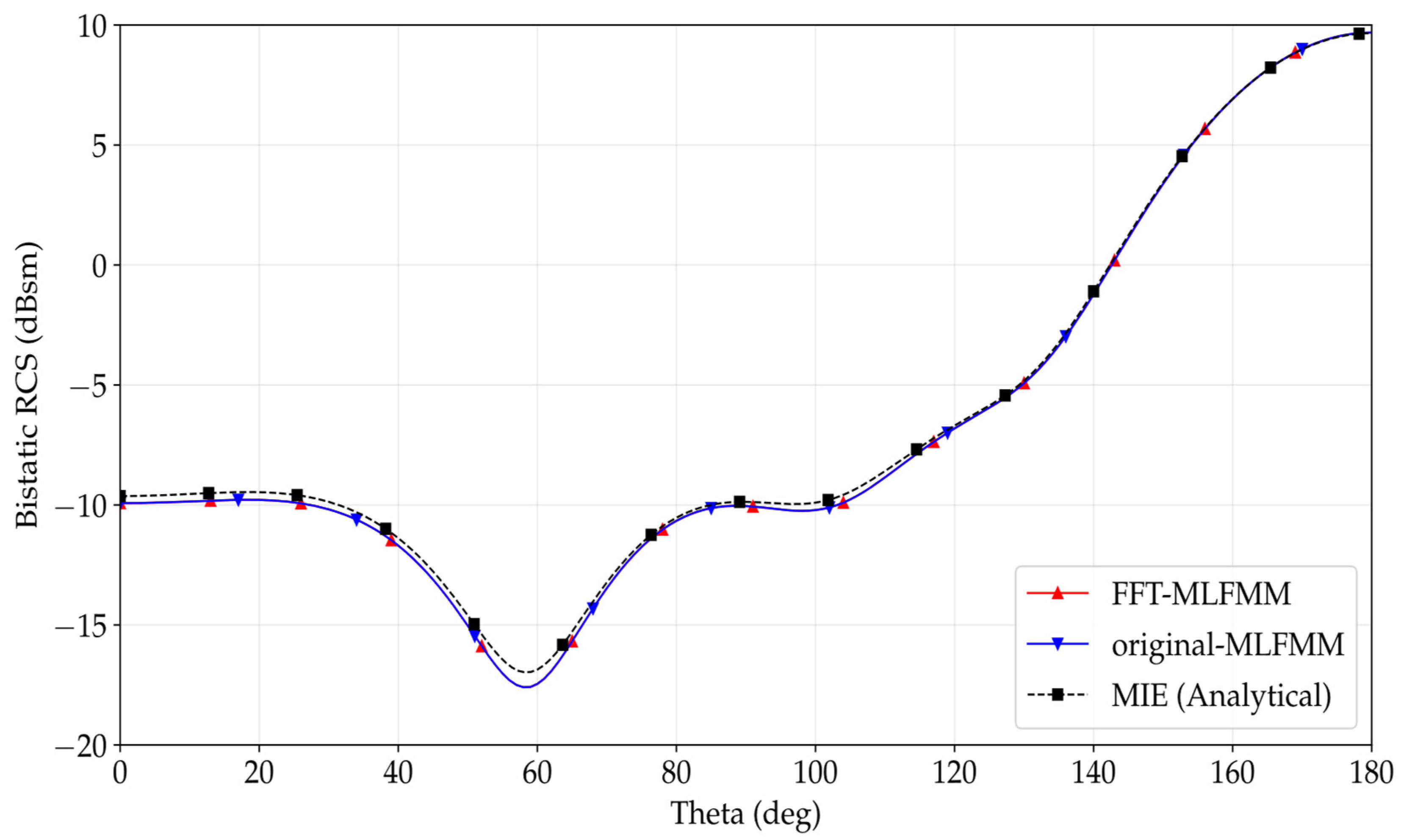
The results obtained show that a significant improvement in the use of computational resources is achieved by the new approach, especially for large cases with a high number of unknowns. The most relevant case in this study is the analysis of 32 div/$\lambda$, as this is a typical value required to obtain accurate results in a meshed dielectric volume. Not only is the memory required reduced from 24.1 GB to 2.3 GB, but also the time required for the computation of a complete iteration is improved (from 1 min to 1 s). However, the most interesting case is observed in the third simulation, illustrating that cases with a considerable number of unknowns are the most efficient for the FFT-based strategy, reducing the total memory required from 1.46 TB to 17.9 GB. The iteration time is also better for the FFT code, because for N = 16, a high number of elements can be computed simultaneously for each region, thus speeding up the computation time per iteration. For the sake of completeness, the bistatic RCS results corresponding to the simulations shown in Table 1 for N = 16 are presented in Figure 2, for a $\theta$ sweep between 0° and 180°. As can be observed, the RCS curves obtained for the code where the rigorous part of the method is computed with FFT show excellent agreement with the curves computed with the analytical code. In addition, the FFT and original computed solutions show very little difference, thus validating the method presented in this work.

A second set of validation cases are now simulated to test the computational cost of the FFT-based code in contrast with the original approach. For these simulations, the objective is to increase the electrical size of the dielectric sphere to analyze the code performance for very large dielectrics and very dense meshes (high number of unknowns with a typical number of 30 divisions per wavelength). For this reason, the physical size of the sphere is fixed, but the analysis frequency is now increased from 0.5 GHz to 3 GHz, thus the electrical size of the sphere is changed from $0.66 \lambda$ to $4 \lambda$ (diameter). The mesh specifications are fixed in all cases to N = 8 for each region, which results in a mesh with 32 divisions per wavelength. Due to the region size becoming smaller as the frequency increases, the number of unknowns is dramatically increased from 0.72 × 10⁶ to 51.23 × 10⁶, as well as the number of regions (from 1638 to 36 × 10³). In these cases, we used the BICGSTAB iterative solver [22] with the exit error set to 0.01 to ensure a good convergence for the solution of the equation system. 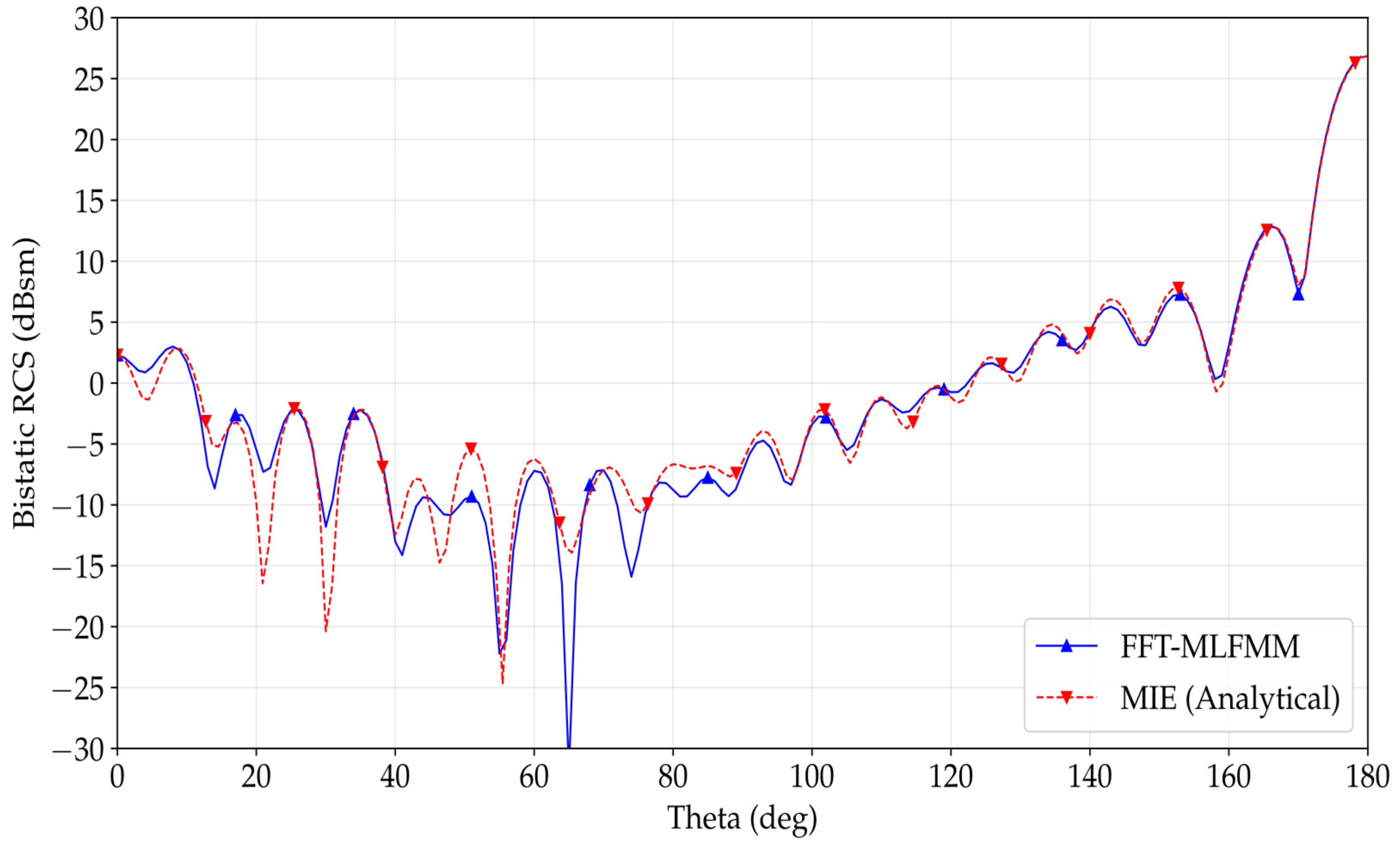Figure 3 shows a comparison of results at 2 GHz obtained using the FFT-MLFMM code and using Mie analytical solution. We immediately notice the good accuracy of the FFT-MLFMM results. The results obtained for this set of simulations are collected in

Table 2. Performance test results corresponding to the homogeneous dielectric sphere simulated at various frequencies.

f	Unknowns	Regions	Iteration Time	Num. Iter	Time per Iter.	Max. RAM
1	1.83 × 106	1638	00:00:39	7	00:00:05	31.885 GB
1.5	6.372 × 106	4992	00:05:27	18	00:00:18	110.15 GB
2	15.143 × 106	11,434	00:19:32	27	00:00:43	254.89 GB
3	51.234 × 106	36,864	01:22:44	43	00:01:44	846.90 GB

. As can be observed, as the simulation frequency becomes higher, the number of unknowns and regions for the problem increase, due to the fixed size of the MLFMM regions at $\lambda /4$. Note that in each simulation the time per iteration increases with the number of regions, which is to be expected, even though the number of divisions per region is fixed in all cases.

5.2. Bistatic RCS of an Homogeneous Sphere with Dielectric Transitions

In order to verify the new formulation introduced in the self-coupling terms for the transitions between dielectrics, the RCS of a homogeneous sphere is computed, with and without the transition between dielectric activated. For this test, a sphere with radius $a={\lambda }_0/2$ is analyzed for a frequency $f_0=300$ MHz. Two meshings are performed over the homogeneous sphere. First, the sphere is meshed without including added mesh hexahedrons at the boundary of the sphere. Second, added mesh hexahedrons are considered. In both cases, a mesh density with $\mathrm{N}=8$ hexahedrons per region is employed (32 divisions per $\lambda$). 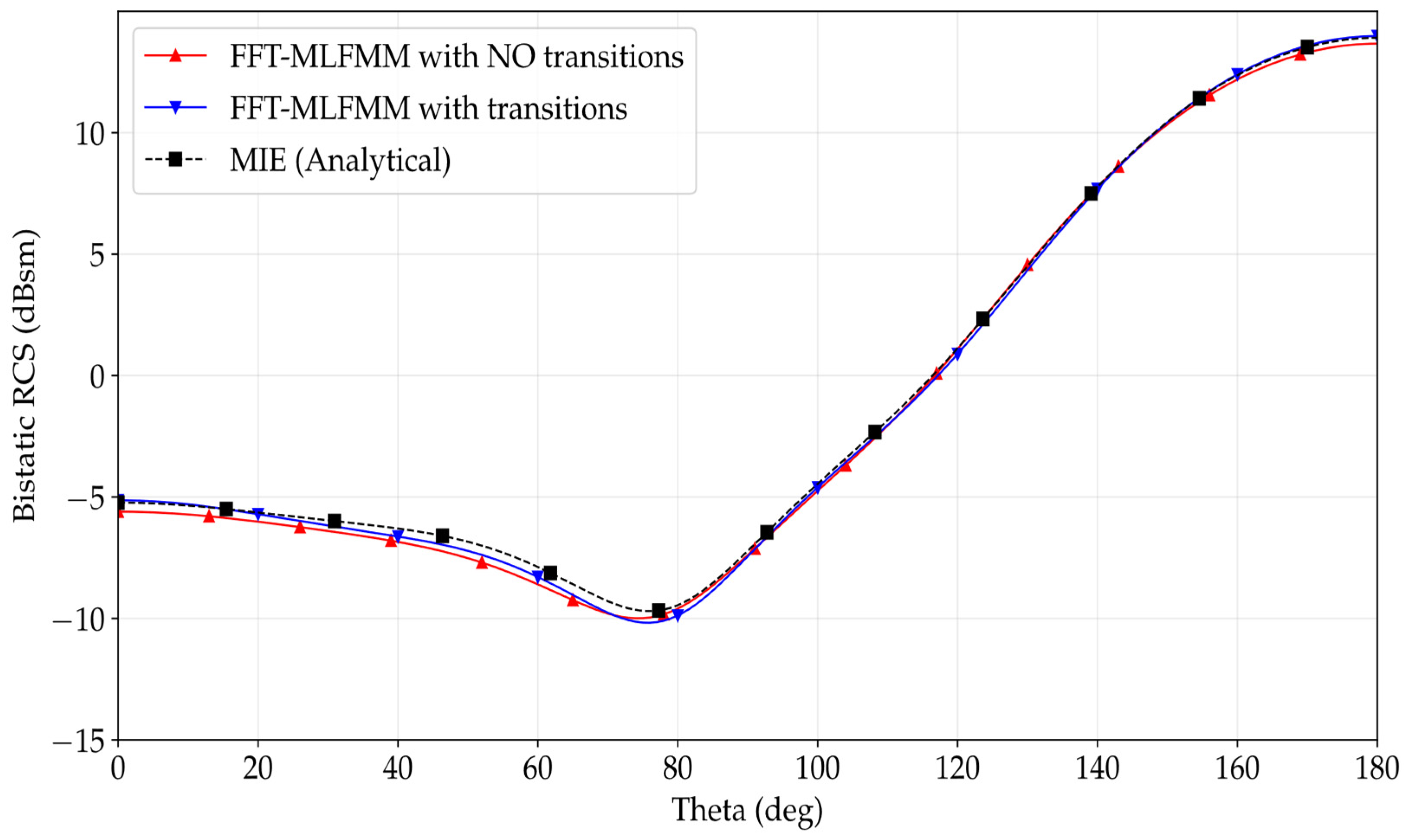The simulation that considers dielectric transitions generates 54,204 unknowns and a total of 75 regions, while the problem without transitions, generates 49,332 unknowns and a total of 64 regions. The results obtained from these two different meshed spheres are compared in Figure 4 with the analytical solution obtained from the Mie formulation for the same sphere. As we can observe in Figure 4, the bistatic RCS from the execution with transitions is slightly more accurate than the execution without transitions. It is clear that including the transitions achieves better accuracies without dramatically increasing the resources required during the computation (in this case, the memory usage and CPU computation times are roughly equal, maximum RAM required is around 1 GB, and time per iteration of the biconjugate solver is less than a second).

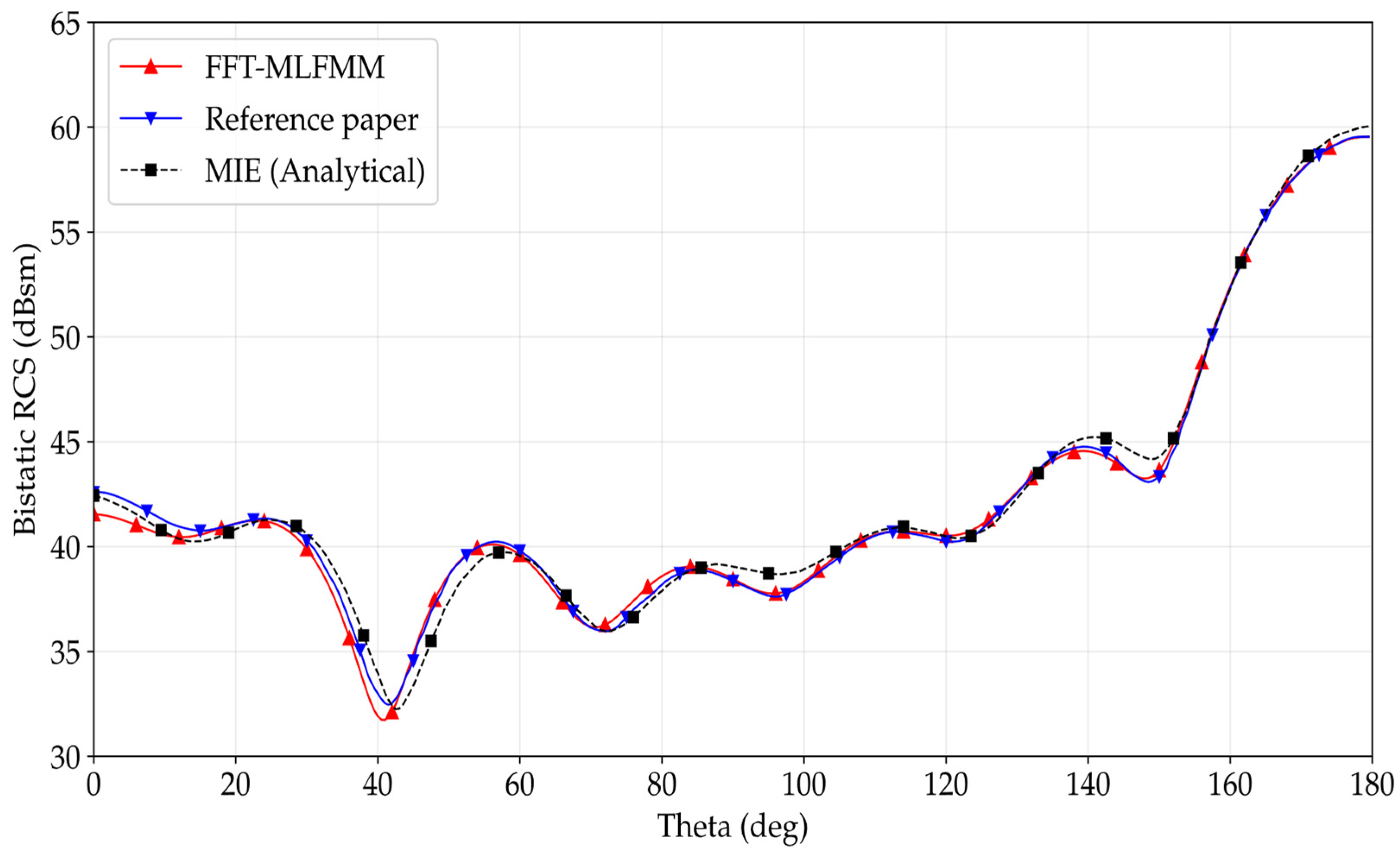
5.3. Bistatic RCS of a Radially Inhomogeneous Dielectric Sphere

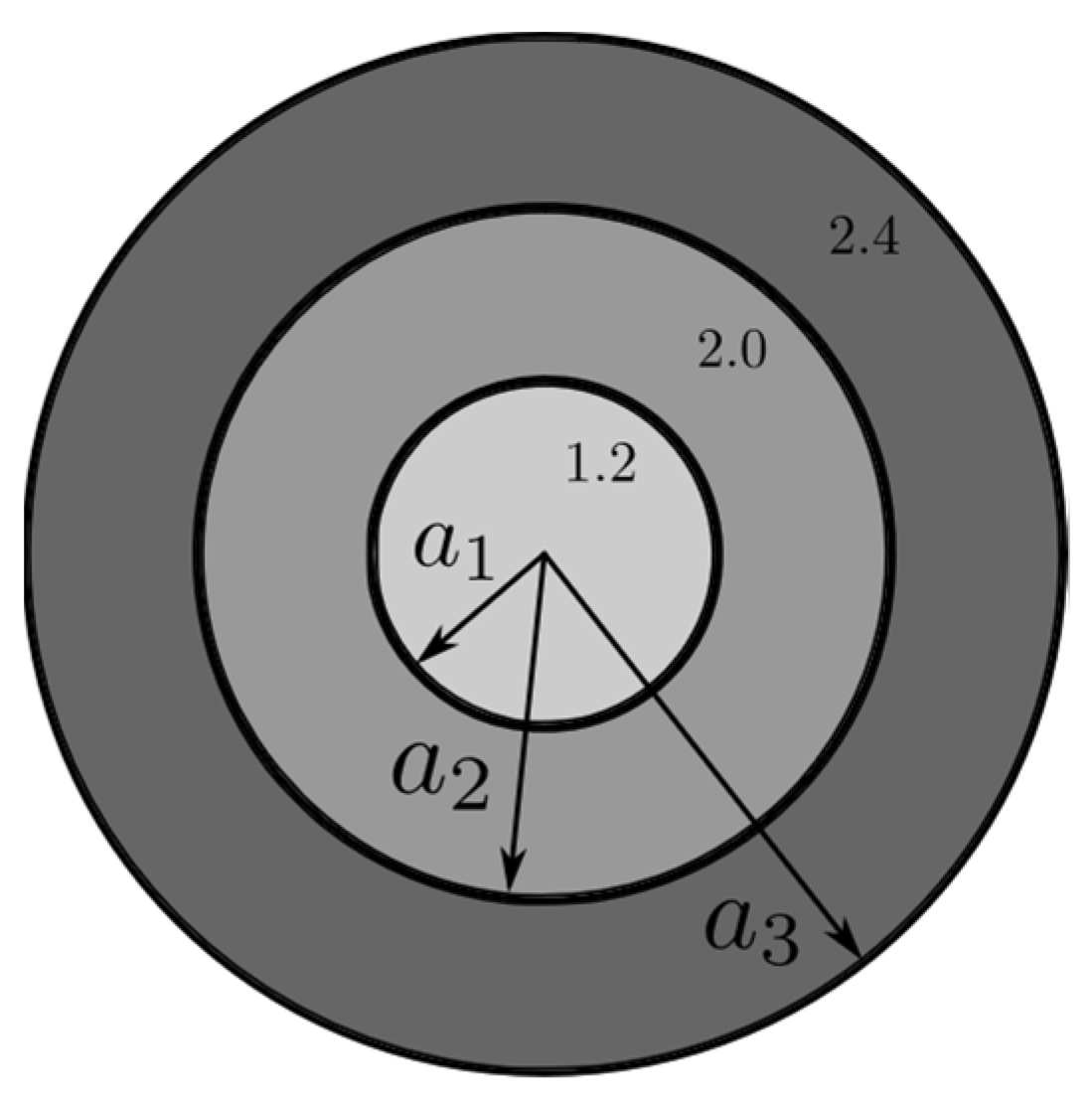
To validate the formulation with transitional mesh elements between dielectrics, an example of a radially inhomogeneous dielectric sphere is simulated. The sphere is divided into 3 layers with radius $a_1,a_2,$ and $a_3$, and each layer has different permittivity, as shown in Figure 5.

The inhomogeneous sphere scattering is computed to calculate the bistatic RCS at $5.9$ MHz. The structure is meshed with $\mathrm{N}=8$ elements per region, resulting in a 32 divisions per wavelength mesh density. This meshing gives a problem with 421,812 unknowns and a total of 441 regions for the MLFMM, for a region size of ${\lambda }_0/4$. The results obtained are compared to those obtained from the analytical Mie formulation for inhomogeneous dielectric spheres and the results obtained in [23]. The comparison between these three RCS computations is presented in Figure 6. The results obtained show a good agreement with the analytical and previously obtained results for the inhomogeneous sphere, thus validating the transitional formulation proposed.

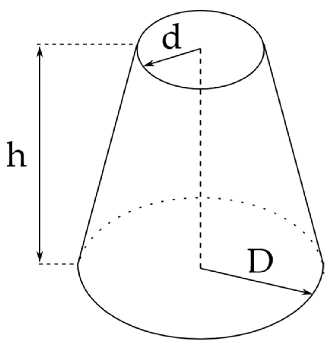
5.4. Bistatic RCS of a Dielectric Conical Frustrum

It is also interesting to verify how the new implementation behaves in a more complex case. A conical frustrum is analyzed, using the dimensions and dielectric permittivity shown in Figure 7.

The results obtained with the FFT-MLFMM program are compared with results obtained with a surface integral equation approach available in FEKO [21]. In all cases, the excitation plane wave is $\theta$ polarized, and the results are shown for the cut-planes with $\phi =0°$ and $0°<\theta <180°$. In the FFT-MLFMM simulation, a meshing of $\mathrm{N}=8$ is chosen, corresponding to 32 divisions per wavelength. The FEKO simulations are configured for a fine mesh setting. The iteration times and RAM consumptions corresponding to the FFT-MLFMM simulations are collected in

Table 3. Performance test results for the analyzed conical frustrum at various frequencies, computed with FFT-MLFMM.

Frequency (GHz)	Unknowns	Regions	Iteration Time	Num. Iter.	Max. RAM
2	102,981	126	<1 s	2	2.0 GB
3	351,068	340	00:00:01	3	6.1 GB
4	836,095	763	00:00:05	4	14.1 GB

.

The results obtained for the lowest analysis frequency are presented in Figure 8. The geometry is meshed with 3782 triangles in FEKO along the surface of the conical frustrum. As can be observed, the RCS curves are very similar, thus a good agreement between both analysis methods is achieved. Note that the simulations with the FFT-MLFMM are performed by considering the transitional mesh hexahedrons corresponding to vacuums throughout the volume of the external surface.

The results for the highest frequency are also presented and compared for both software simulations in Figure 9. In this case, the geometry is meshed with 14,994 triangles in FEKO along the surface of the conical frustrum. As in the previous comparison, the responses between the two software packages are very similar, even though some differences are observed in the cuts for $55°<\theta <100°$.

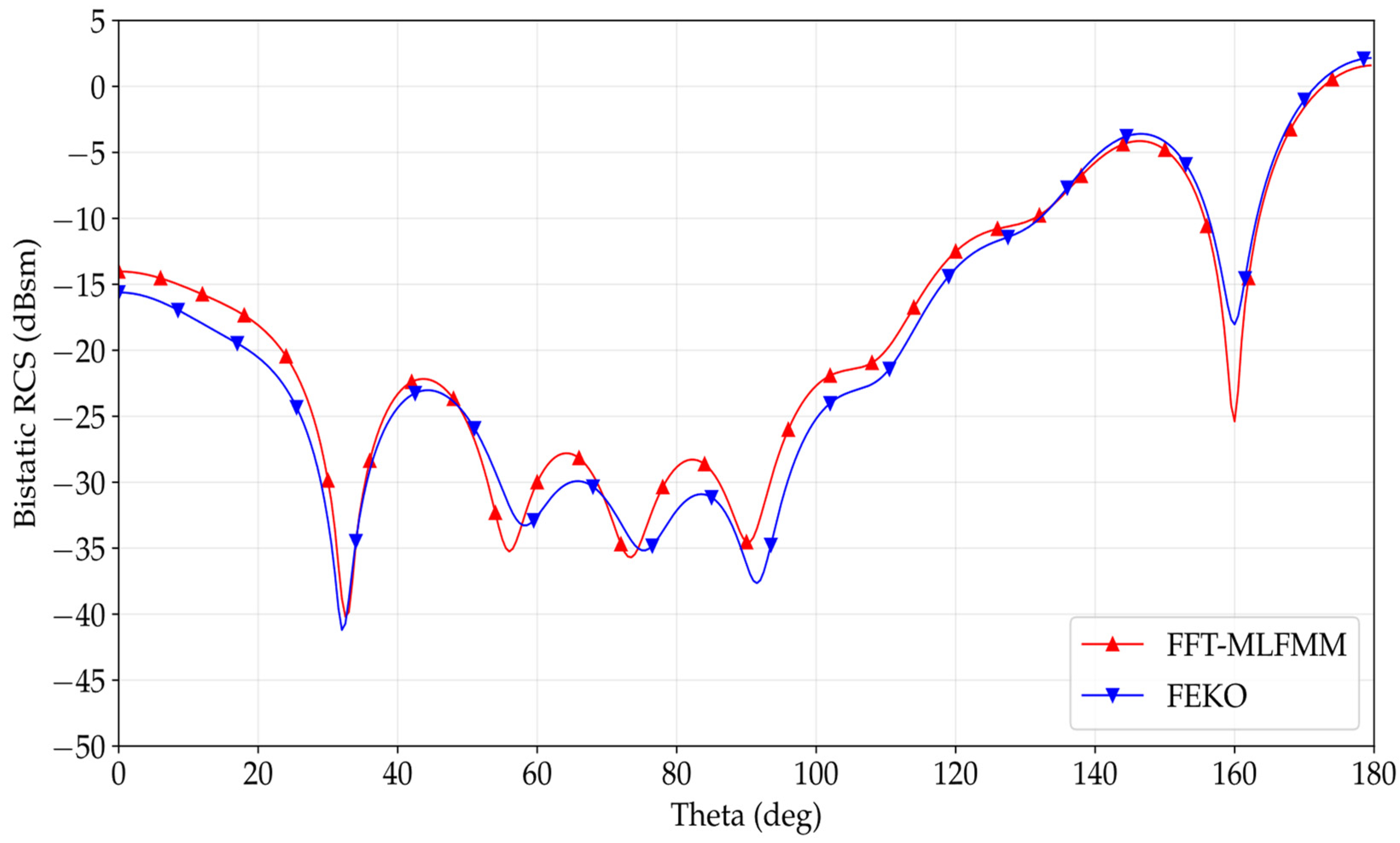
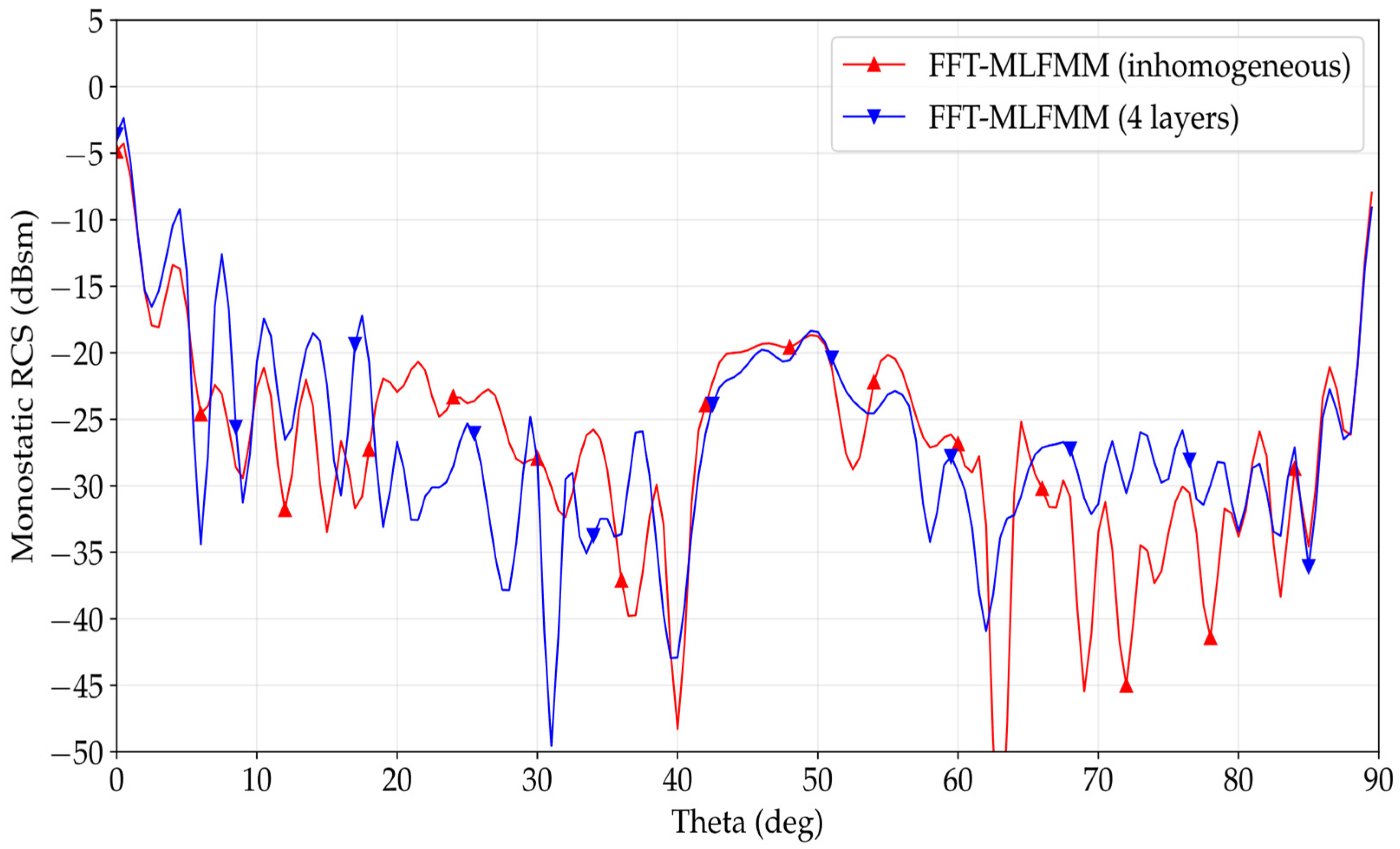
5.5. Monostatic RCS of a Radially Inhomogeneous Cylinder

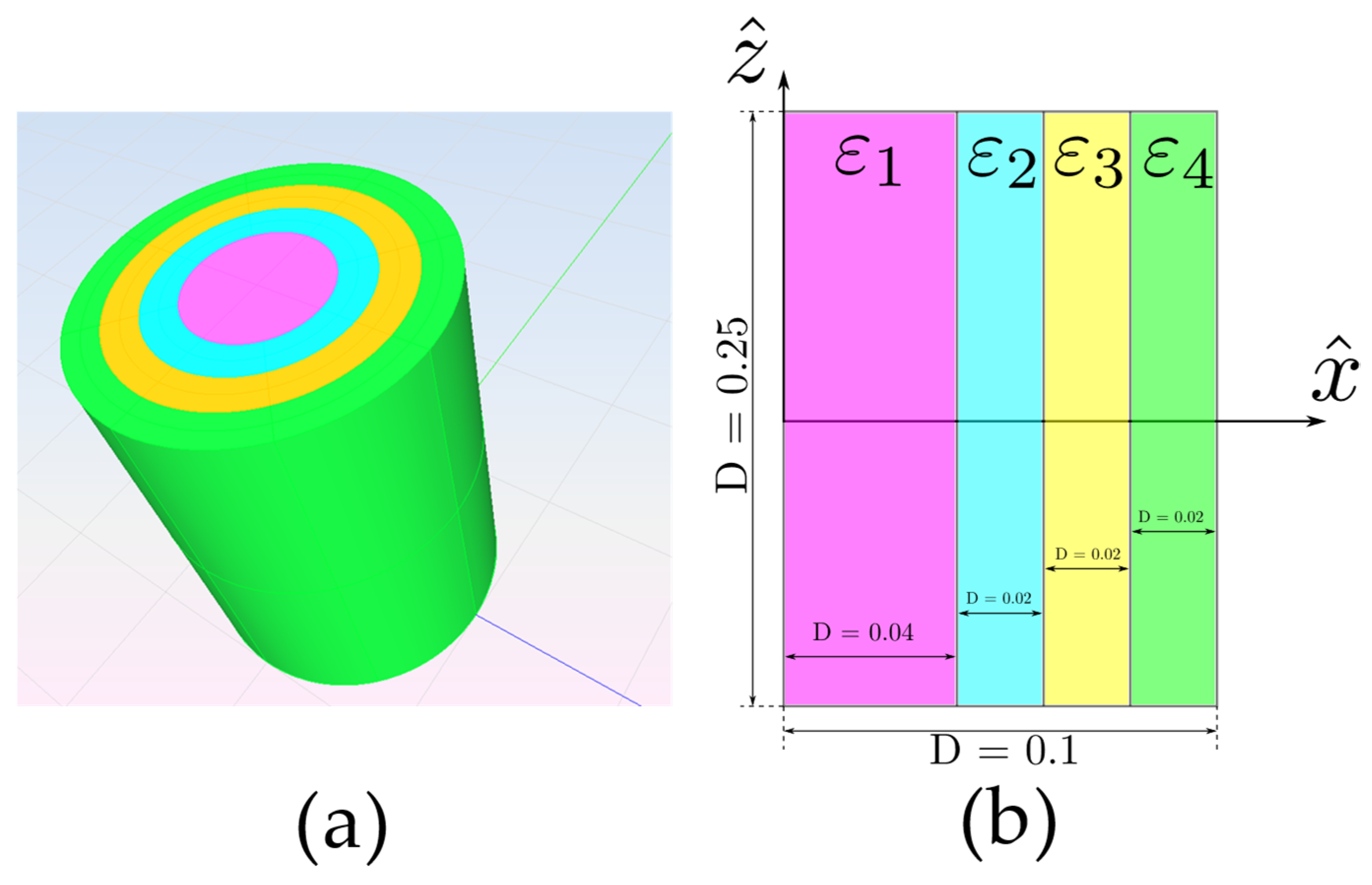
The transitional mesh formulation has also been tested with non-analytical geometries. In this section, the monostatic RCS of an inhomogeneous cylinder is analyzed for two different cases. In the first case, the dielectric permittivity is defined as a four-layer cylinder with radially homogeneous permittivity inside each layer. In the second case, the inhomogeneous dielectric permittivity is defined using a continuous function.

The physical geometry for the inhomogeneous cylinder, composed of four dielectric layers, is shown in Figure 10. This cylinder is composed of four dielectric layers. The dielectric permittivity corresponding to each layer is: ${\epsilon }_{r1}=0.895-j0.021$, ${\epsilon }_{r2}=1.097-j0.019,$ ${\epsilon }_{r3}=1.431-j0.015,$ and ${\epsilon }_{r4}=1.788-j0.012$. The frequency is $f_0=15 \mathrm{GHz}$, and the meshing considers eight divisions per $\lambda$. This low mesh density is justified by the low permittivity values of each layer, which are very close to the vacuum ${\epsilon }_r=1$.

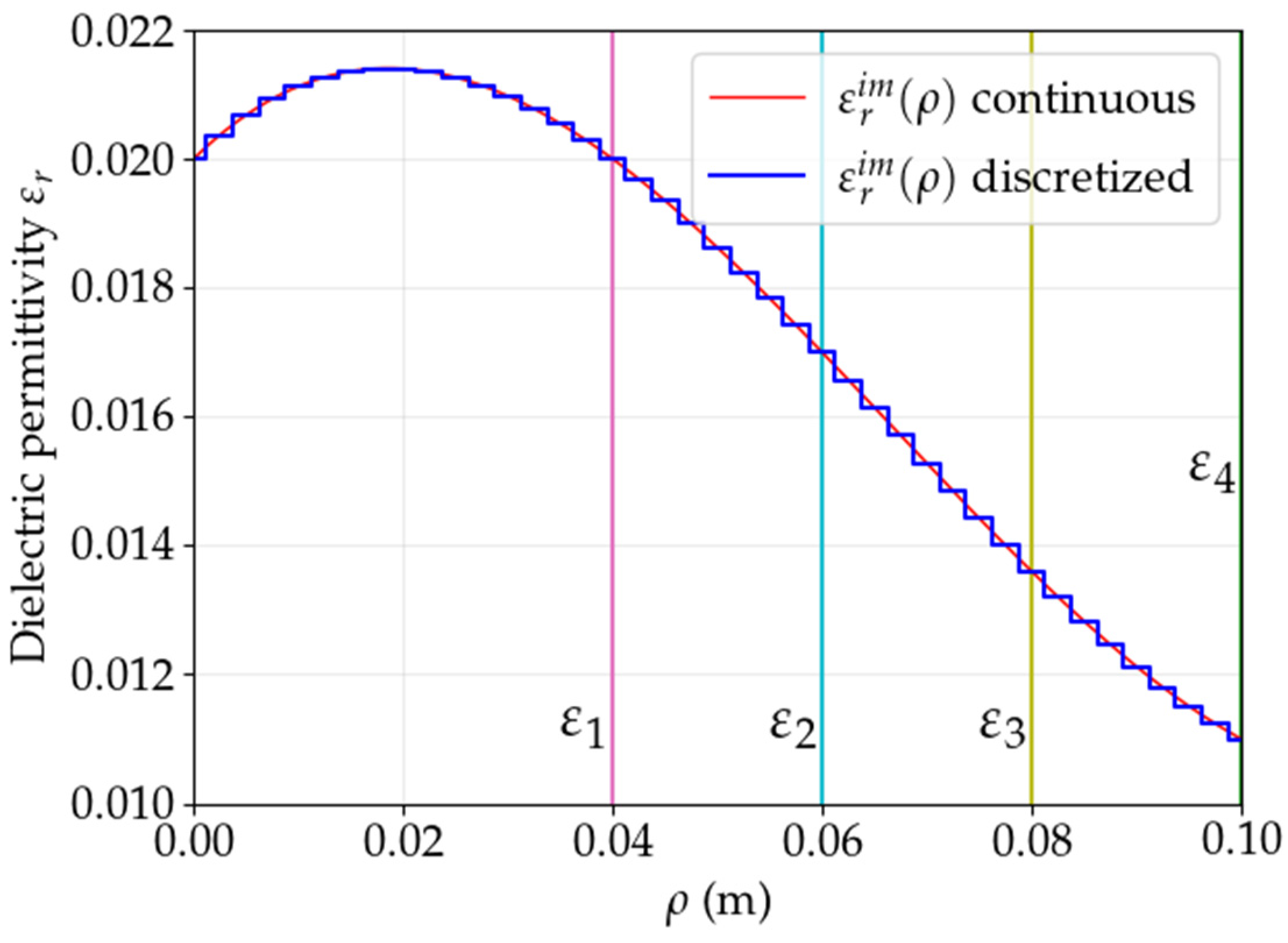
In the second case, the four layers are replaced by a single volume with the dielectric permittivity defined by a continuous mathematical expression. The dielectric permittivity is defined as a function of the distance $\rho$ between the point and the cylinder $\widehat{z}$ axis, as

$${\epsilon }_r\left(\rho \right)={\epsilon }_r^{re}\left(\rho \right)-j{\epsilon }_r^{im}\left(\rho \right)$$

(15)

where

$${\epsilon }_r^{re}\left(\rho \right)=1-16\rho +464{\rho }^2-2083{\rho }^3$$

(16a)

$${\epsilon }_r^{im}\left(\rho \right)=0.02+0.16\rho -5{\rho }^2+25{\rho }^3$$

(16b)

We assign to each mesh element the dielectric permittivity given by expressions (16) evaluated at the center of the hexahedron. By doing this, the continuous function of the dielectric permittivity is discretized according to the hexahedral mesh of the geometry. Figure 11 and Figure 12 show a comparison between the continuous and the discretized variations of the dielectric permittivity. The mesh density in both cases is similar, with $\mathrm{N}=2$ (8 divisions per wavelength). Note that, from the simulation point of view, the only difference between the two cases lies in the assignation of the dielectric permittivity to the hexahedron mesh elements.

The problem has about 1.5 million unknowns and about 66 thousand regions (with a region size of $\lambda /4$). For the iterative solver, the GMRES algorithm is chosen, with a relative error of 0.01 to stop the iterations. We have computed monostatic RCS for the $\phi =0°$, for $0°<\theta <90°$, considering $\theta$ steps of 0.5°. It takes about 7 s to compute each individual iteration for the solution of each direction, and the maximum RAM usage is about 59 GB. Each solution cut direction converges on about 200 iterations.

The first simulation is for $\theta$-polarized incidence and the results obtained for both inhomogeneous cylinders are presented in Figure 13. Even though these two cylinders are not exactly equal, due to their dielectric permittivity definition, similarities are observed, especially for the lower values of $\theta$. For the sake of completeness, an additional pair of simulations is presented in Figure 14, for a $\phi$-polarized incidence. Similar commentaries to those provided for the results already obtained can be applied to these results.

6. Conclusions

A scheme based on FFT is proposed for the computation of the near-field coupling in the iterations of the multi-level fast multipole method (MLFMM) for the analysis of large dielectric problems with complex geometries. The scheme is efficient for the analysis of large homogeneous and non-homogeneous dielectric volumes. In addition, we propose a new approach for the numerical treatment of the transition of the relative dielectric permittivity between different dielectrics or between a dielectric and the free space. The scheme is validated considering RCS results of several cases with homogeneous and non-homogeneous dielectric bodies. Future extensions of the approach developed here will consider the case of arbitrary dielectrics close to or with imbibed metallic surfaces, which is very interesting for engineering applications.