Chaos Suppressing in a Three-Buses Power System Using an Adaptive Synergetic Control Method

Abstract

The stability of the power system is a critical issue for the reliable and safe operation of the network. Where maintaining voltage levels constant or within the prescribed permissible limit and robustness against disturbances, while the power system is working near its stability margin due to growth of power consumption, nowadays are great challenges. Chaotic oscillation in power network may lead to system bus voltage collapse, angle divergence and possibly both phenomena simultaneously. These cases directly affect the service quality of the power system. The paper presents the problem of chaos suppressing in a three-bus power system of a six-dimensional model. The dynamics of the power system are investigated through examining the nonlinear system’s behavior analysis tools, such as power spectral density, bicoherence, Poincaré map and the Lyapunov exponents. The chaotic oscillation of the power system is suppressed through a Lyapunov-based adaptive algorithm with synergetic control theory. A nonlinear evolution constraint is used for achieving better transient responses and fast dynamics. The dynamics of the energy storage device and STATCOM compensator are employed within the control loop to restore the synchronous operation and maintain the rated voltage, respectively. Numerical simulations are conducted to verify the effectiveness and robustness of the proposed control algorithm. The stabilization of the chaotic power system dynamics and the fast recovery to the normal state are characterized by a smooth and free-of-chattering controller output.

1. Introduction

Power system voltage stability is the ability of the power system to maintain stable voltages within the rated value for all power system buses at all operating conditions, even after undergoing some disturbance effects. Disturbances can be due to demand load change, system faults, or any other issues affecting the system stability. Disturbances in the power system, may force the power system to suffer from voltage instability, and causes an uncontrollable progressive change in the voltages of the system buses. Consequently, this leads to an unacceptable voltage service quality in different parts of the power network and possibly leads to a voltage collapse or a voltage avalanche [1]. It is important to mention that the tripping of power transmission lines and/or losses of system loads and the complete shutdown of the affected areas may follow a voltage collapse [2].

Chaos is a nonlinear complex phenomenon that can critically affect the dynamical systems stability behavior. Unpredictability, high sensitivity to initial conditions consequently yielding completely different responses [3], are the main attributes of chaotic systems that led to severe blackouts and power system failures [4]. It can be induced by parameter variations [5], time delay [6] and external disturbances [7]. Chaos has been widely investigated in many systems in different areas [8,9]. Control of chaotic systems in engineering and science is currently an interesting research area in the modern control literatures [10].

The chaotic phenomena in power systems have been analyzed by several researchers. One of the first studies are those of Chiang et al. [11,12] in the early 1990s, where they studied the chaotic behavior of a two-bus simple interconnected power system under different load conditions. Early studies mainly focused attention on interpreting the chaotic oscillation behavior of power systems [13,14,15]. Routes to chaos and the relationship between power system instability and chaotic oscillation were presented by [16]. The scholars in [17] showed that chaos can force a voltage profile of the power system to instability then to collapse when stability conditions are ruined. In addition, it was reported that chaos occurs possibly as an intermediate case in the instability state after a large disturbance affecting the power system. In [18], it was revealed that the collapse of voltage is related to static bifurcation and/or dynamic bifurcation. Moreover, it was shown that the nominal operating point subjected to dynamic bifurcations prior to the static bifurcation for which voltage collapse was attributed. Chaotic power oscillation occurs in the electrical network due to many other phenomena. Subsynchronous resonance (SSR) and ferroresonance are two phenomena that cause power oscillation of rotary systems. During SSR, electrical energy is exchanged between the generation unit and transmission systems with a frequency below the fundamental synchronous frequency. It happens due to electro–mechanical interactions of a series-compensated transmission line with a generator. It results in oscillation in the shaft and power oscillation [19,20]. Ferroresonance is a nonlinear resonance, which occurs in the presence of a saturable nonlinear inductance and capacitance in a circuit with low resistance. It can emerge due to several configurations, like breaker failure during opening or closing operation, line and plant outage, etc. It causes a misshaping of the waveforms, power oscillation and frequency deviation in the network [21,22]. Obviously, chaotic oscillations are harmful to power systems and should be suppressed or eliminated by using effective control measures. Several control methods have been developed for this purpose. Since power systems are highly nonlinear, different nonlinear control strategies have been developed for chaotic oscillation suppression and elimination in power systems. Global state feedback linearization has been developed in [23] to suppress chaotic oscillations in the power system. Moreover, adaptive control algorithms have been applied for chaos control of power systems in [24,25]. In addition, [25] applied a conventional linear manifold synergetic controller that suffers from the problem of a long convergence time to the equilibrium point, and reaching the reference signal may not be fast enough in cases that the initial conditions of the system state variables are far from the equilibrium [26].

Several types of sliding mode control (SMC) strategies have been developed for chaos control and avoiding power system voltage collapse [27,28]. However, the main obstacle for the SMC practical engineering implementation, is an undesirable phenomenon associated with the sliding mode theory known as the chattering. The chattering is a harmful oscillation of a finite frequency and amplitude. This devastating phenomenon distinctly affects the controller accuracy and can lead to damage in the actuator mechanical moving parts of the controlled system, besides high power circuit losses. Chattering can amplify the neglected system fast dynamics during the ideal modeling moreover, it induces instability problems [29]. Although there are different methods to overcome the chattering phenomenon problem, including, but not limited to SMC approximations [30] and application of high order sliding mode (HOSM) [31]. Most of these approaches reduce the chattering to different degrees at the expense of reducing robustness and added complexity.

These facts illustrate the necessity of finding a fundamental new control approach such as the synergetic control theory, instead of traditional ones. This new method is characterized by the use of robust control for the multi-connected nonlinear mathematical models, to satisfy the practical implementation of the required invariant manifolds, or attractors, and enhance the controlled system stability. The synergetic control principles are based on the analytical design of aggregated regulators (ADAR) [32]. The approach uses a totally smooth continuous control law to remove the chattering phenomena and insures the same closed-loop invariant level as in the SMC.

Therefore, the synergetic control theory has attracted a great deal of attention. Where it has been successfully used in many industrial applications such as power electronics, power systems, quadrotor helicopter system, grid-connected photovoltaic systems, and robotic manipulators, are all applications reported in the literature [33]. The fundamental principles of synergetic control are based on the theory of directed self-organization [26]. Synergetic control theory was first proposed by the Russian researcher Kolesnikov [32]. Where the problem of the system synthesis i.e., finding the objectives for the common process control of the nonlinear dynamical system, is handled based on the synergetic realization [32]. The synergetic control scheme has the merit of employing the complete input-output nonlinear dynamical model and does not need a model linearization or simplification, as it common in the traditional control methods [34]. From the practical applicability point of view, the synergetic control has several advantages. First, it is well-suited for digital control implementation as it needs a fairly low bandwidth for the controller. On the other hand, the SMC needs a fairly high bandwidth for the controller, which hinders the solution feasibility. The second advantage is that it requires a constant switching frequency and it does not have chattering problems, therefore it causes fewer power filtering problems in power electronics applications [33].

Motivated by the above discussion, this paper presented the following aspects: suppressing chaotic oscillation in a six-dimensional power system. Employing static synchronous compensator (STATCOM), which is a superior technology in supporting system bus voltage against large-scale disturbances [35]. It has the advantage of fast voltage recovery which is crucial to maintain the power system transient voltage stability [36]. Moreover, an energy storage device has been exploited along with synergetic control theory based on an adaptive control algorithm and nonlinear evolution constrain approach, to elaborate a robust control scheme for stabilizing the power system dynamics.

This paper consists of six sections. Following this introduction, Section 2, introduces the mathematical model of the chaotic power system. In Section 3, the synergetic control theory fundamentals are presented along with the general control framework. In Section 4, the adaptive synergetic controller design for the chaotic power system is presented. In Section 5, the dynamical behavior of the power system is investigated through nonlinear analysis tools such as Poincaré map, system trajectory evolution, power spectral density and bicoherence to reveal the chaotic nature of the power system. Then, three simulation procedures were provided to verify the controller robustness and effectiveness. The main conclusions and discussion are presented in Section 6.

2. Mathematical Model

In this section, the dynamic behavior of the chaotic power system model [25,37], is investigated. The system can be regarded as one generator bus 1 supplying power to a local load bus 2 and connected to slack bus 3, as shown in Figure 1. The dynamics of the system depend on the generator angle ${\delta }_m$, generator slip $s_m$, the generator q-axis transient potential $E_q^{{}^{\prime }}$, excitation potential $E_{fd}$, the load phase angle ${\delta }_L$ and $V_L$ the load bus voltage amplitude as written in (1).

$$\begin{array}{c}\hfill \left\{\begin{array}{cc}{\displaystyle {\dot{\delta }}_m}\hfill & ={\omega }_B{s}_m,\hfill \\ \\ {\displaystyle {\dot{s}}_m}\hfill & {\displaystyle =\frac{1}{2H}\left(-d{s}_m+P_m-P_g\right),}\hfill \\ \\ {\dot{E}}_q^{{}^{\prime }}\hfill & {\displaystyle =\frac{1}{T_{d0}^{{}^{\prime }}}\left(-E_q^{{}^{\prime }}+(x_d-x_d^{{}^{\prime }})I_d+E_{fd}\right),}\hfill \\ \\ {\dot{E}}_{fd}\hfill & {\displaystyle =\frac{1}{T_A}\left(-E_{fd}+K_A(V_{ref}-V_t)\right),}\hfill \\ \\ {\dot{\delta }}_L\hfill & {\displaystyle =\frac{1}{q_1}\left(Q-Q_{1d}-Q_0-q_2{V}_L-(q_3-B_c)V_L^2\right)}\hfill \\ \\ {\dot{V}}_L\hfill & {\displaystyle =\frac{1}{p_2}\left[P-P_{1d}-P_0-p_3{V}_L-\frac{p_1}{q_1}\left(Q-Q_0-Q_{1d}-q_2{V}_L-(q_3-B_c)V_L^2\right)\phantom{\frac{1}{2}}\right].}\hfill \end{array}\right.\end{array}$$

(1)

All parameters in the model (1) are considered as constants, except the functions $P_g$, P, Q, $I_d$ and $V_t$ that depends on the power system model state variables. $P_g$ parameter defines the power delivered by the generator, and can be written as:

$$P_g=(x_d^{{}^{\prime }}-x_q)I_d{I}_q+E_q^{{}^{\prime }}{I}_q,$$

(2)

where

$$\begin{array}{c}\hfill \left\{\begin{array}{cc}{I}_d\hfill & =[(Y{E}_q^{{}^{\prime }}-a)(sin\varphi -Y{x}_q)-bcos\varphi ]/A,\hfill \\ I_q\hfill & =[(Y{E}_q^{{}^{\prime }}-a)cos\varphi +(sin\varphi -Y{x}_d^{{}^{\prime }})b]/A\hfill \end{array}\right.\end{array}$$

(3)

and

$$\begin{array}{c}\hfill \left\{\begin{array}{cc}A\hfill & =\left[{cos}^2\varphi +\left(sin\varphi -Y{x}_q\right)\left(sin\varphi -Y{x}_d^{\prime }\right)\right],\hfill \\ a\hfill & =Y_3{E}_{b}cos\left({\delta }_m-{\varphi }_3+\varphi \right)+V_L{Y}_{1}cos\left({\delta }_L-{\delta }_m+{\varphi }_1-\varphi \right),\hfill \\ b\hfill & =-Y_3{E}_{b}sin\left({\delta }_m+\varphi -{\varphi }_3\right)+V_L{Y}_{1}sin\left({\delta }_L-{\delta }_m+{\varphi }_1-\varphi \right),\hfill \\ Y\hfill & =\sqrt{Y_1^2+Y_3^2+2Y_1{Y}_{3}cos\left({\varphi }_1-{\varphi }_3\right)},\hfill \\ \varphi \hfill & ={tan}^{-1}\left[\frac{Y_{1}sin{\varphi }_1+Y_{3}sin{\varphi }_3}{Y_{1}cos{\varphi }_1+Y_{3}cos{\varphi }_3}\right].\hfill \end{array}\right.\end{array}$$

(4)

where $I_d$ and $I_q$ represent components of stator current on the d-axis and the q-axis, respectively. The expressions for the load active power P, reactive power Q and the generator bus terminal voltage $V_t$ are defined as (5):

$$\begin{array}{c}\hfill \left\{\begin{array}{cc}P=\hfill & V_L{V}_t{Y}_{1}cos\left({\beta }_1\right)-Y_1{V}_L^{2}cos\left({\varphi }_1\right)+V_L{E}_b{Y}_{2}cos\left({\beta }_2\right)-Y_2{V}_L^{2}cos\left({\varphi }_2\right)\hfill \\ Q=\hfill & V_L{V}_t{Y}_{1}sin\left({\beta }_1\right)+Y_1{V}_L^{2}sin\left({\varphi }_1\right)+V_L{E}_b{Y}_{2}sin\left({\beta }_2\right)+Y_2{V}_L^{2}sin\left({\varphi }_2\right)\hfill \\ V_t=\hfill & \sqrt{{\left(V_d\right)}^2+{\left(V_q\right)}^2}\hfill \end{array}\right.\end{array}$$

(5)

where

$$\begin{array}{c}\hfill \left\{\begin{array}{cc}{V}_d\hfill & =-x_q{I}_q\hfill \\ V_q\hfill & =E_q^{\prime }+x_d^{\prime }{I}_d\hfill \\ {\beta }_1\hfill & ={\delta }_L-\theta -{\varphi }_1\hfill \\ \theta \hfill & ={\delta }_m+{tan}^{-1}\left(\frac{V_d}{V_q}\right)\hfill \\ {\beta }_2\hfill & ={\delta }_L-{\varphi }_2\hfill \end{array}\right.\end{array}$$

(6)

3. Synergetic Control Theory

The synergetic control method is an attractive trend in control science [38]. It found particular applications in nonlinear systems for solving complicated controlling problems. Synergetic control theory (SCT) needs a comprehensive view of controlled system dynamic interactions between energy, matter and information being implemented using positive and negative feedback [39]. The synergetic control method is based on the principle of expansion and contraction of the controlled system state space. It can achieve the required transient performance, which is a challenging requirement for modern control of nonlinear system [26]. The control objective of this paper is to design an adaptive synergetic control algorithm for power system dynamics stabilization. The following preliminary definitions are provided:

Consider the following nonlinear system:

$$\begin{array}{c}\hfill \left\{\begin{array}{cc}{\dot{x}}_i\hfill & =x_{i+1},i=1,2,\cdots ,n-1\hfill \\ {\dot{x}}_n\hfill & =f_n\left(x\right)+g_n\left(x\right)u\hfill \end{array}\right.\end{array}$$

(7)

where $x\in R^n$ is the system states vector, $f_n\left(x\right)\in R$ is a smooth function that denotes the nonlinear dynamics of the system. The gain control function is designated by $g_n\left(x\right)\ne 0$, and $u\in R$ is the control signal. The calculated continuous synergetic control law u, drives controlled system states to a prescribed invariant manifold and then onto the operating equilibrium point of the system (7). The main advantage of this method is that once system dynamics reach the invariant manifold, the system states remain insensitive to parameter variation and disturbances. The synergetic control law u is a function of an aggregated variable of system states called the macro variable $\psi$. These macro variables $\psi$ should be chosen properly by the designer to satisfy the following evolution constrain (8) [40,41]:

$$T\dot{\psi }+\Omega (\psi )=0,$$

(8)

where T determines the macro variable $\psi$ rate of convergence to the synergetic attractor $\psi (x,t)=0$, and $\Omega (\psi )$ is a differentiable smooth function of $\psi$ that is selected such that:

(a)

invertible and differentiable;

(b)

$\Omega \left(0\right)=0$;

(c)

$\Omega (\psi ).\psi >0,\forall \psi \ne 0$.

Lemma 1.

If $\Omega (\psi )$ is designed in the form of (9), then the function $\Omega (\psi )$ satisfies previous conditions [42].

$$\Omega (\psi )={\psi }^{(m_1/n_1)}+{\psi }^{(n_1/m_1)}$$

(9)

where $m_1>0$ and $n_1>0$, are odd numbers and satisfy $0<n_1/m_1<1$.

Proof. 

The proof can be found in Appendix A. □

Then the synergetic nonlinear evolution constrain can be described by the following form (10):

$$T\dot{\psi }+{\psi }^{(m_1/n_1)}+{\psi }^{(n_1/m_1)}=0,$$

(10)

where the design parameters $m_1$, $n_1$ and T are chosen such that the macro variable $\psi$ reaches the synergetic invariant manifold as fast as required. From the synergetic point of view, these parameters are related to actions done by self-organization forces. Where an appropriate selection for these parameters can determine the required speed of self-organization process.

An attractive advantage of the nonlinear synergetic manifold is the appropriate transient response of the controller, which is one of the important issues in the modern controller design process. In the conventional synergetic controller with linear manifold, in cases that the system initial conditions are far from equilibrium, the time of convergence to the reference value may not be rapid enough. In contrast, in the synergetic control with the nonlinear exponential functional constrain (10), with a proper setting of the exponential term parameters, it is possible to drive the system dynamics, from any bounded initial state to the equilibrium, and keep them there. Based on the synergetic control theory properties, this movement to the steady-state will have smooth, proper conditions with a rapid convergence rate. The object of the controller is to restore the state variables of the chaotic power system (1) to the required states and stabilize the system dynamics.

4. Synergetic Based Adaptive Controller Design for the Chaotic Power System

To suppress the chaos in the power system (1) and get rid of the chaotic oscillation and restore the normal operation. It is important to force the power system dynamics to work in synchronization and keep the bus voltage within the required limit. In this work, the objective of the designed controller is achieving ${\delta }_{md}=s_{md}=0$ and $,V_{Ld}=1$ and keep the system in the equilibrium state. To enhance power system stability and achieve the desired control objectives, two facilities will be simultaneously used, which are the energy storage system and the STATCOM compensator. The dynamical model of these two systems, energy storage device [43] and the STATCOM [35], are given as follows:

$$\begin{array}{c}\hfill \left\{\begin{array}{cc}{\dot{P}}_{es}\hfill & =-\frac{1}{T_{es}}{P}_{es}+\frac{K_{es}}{T_{es}}{u}_{es}\hfill \\ \\ {\dot{i}}_{stat}\hfill & =-\frac{1}{T_{stat}}{i}_{stat}+\frac{K_{stat}}{T_{stat}}{u}_{stat}\hfill \end{array}\right.\end{array}$$

(11)

where $P_{es}$ represents the amount of the active power handled by the energy storage system. $T_{es}$ represents energy storage device time constant. $K_{es}$ represents the gain of the input control signal. $u_{es}$ denotes the input control signal. $i_{stat}$ denotes the STATCOM compensator current, $T_{stat}$ defines the STATCOM time constant, $K_{stat}$ designates the input gain and $u_{stat}$ denotes the input control signal.

It is known that energy storage devices have been considered by many researchers as oscillation damping units in power system [44]. The damping of active power oscillations is more effective through active power modulation. The energy storage device can provide real power, therefore it can damp out oscillations very effectively when its output is modified by a proper control algorithm. Therefore, the energy storage device is used to dampen out the oscillation in the system (1) and restore synchronous state using the control signal $u_{es}$. On the other side to keep the bus voltage at rated, the STATCOM compensator is employed through the control input signal $u_{stat}$.

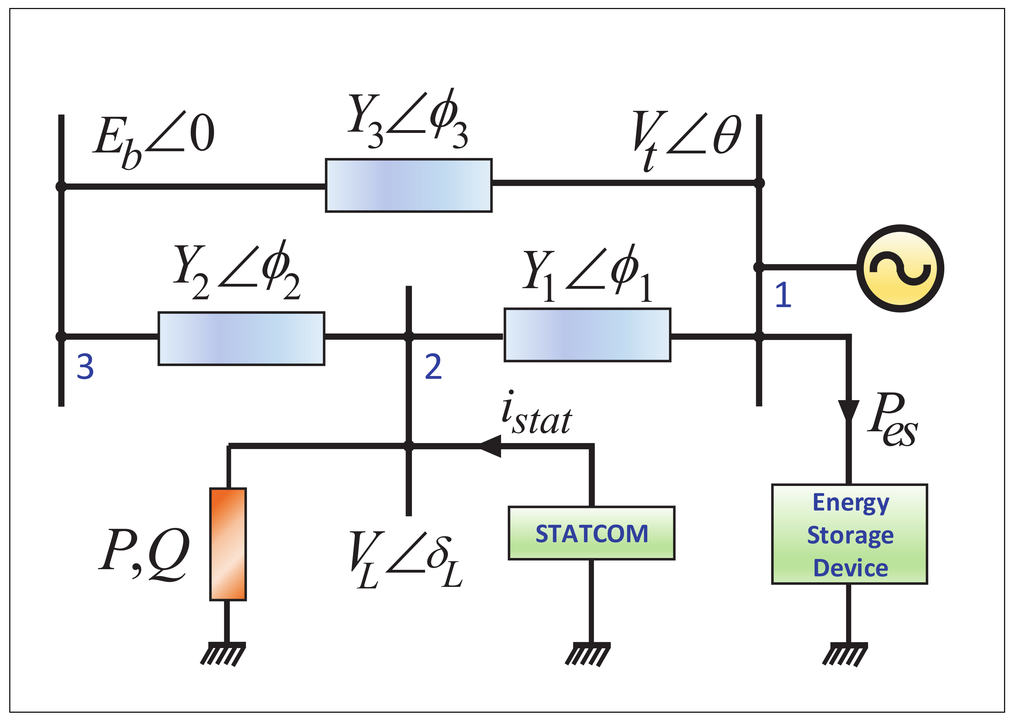
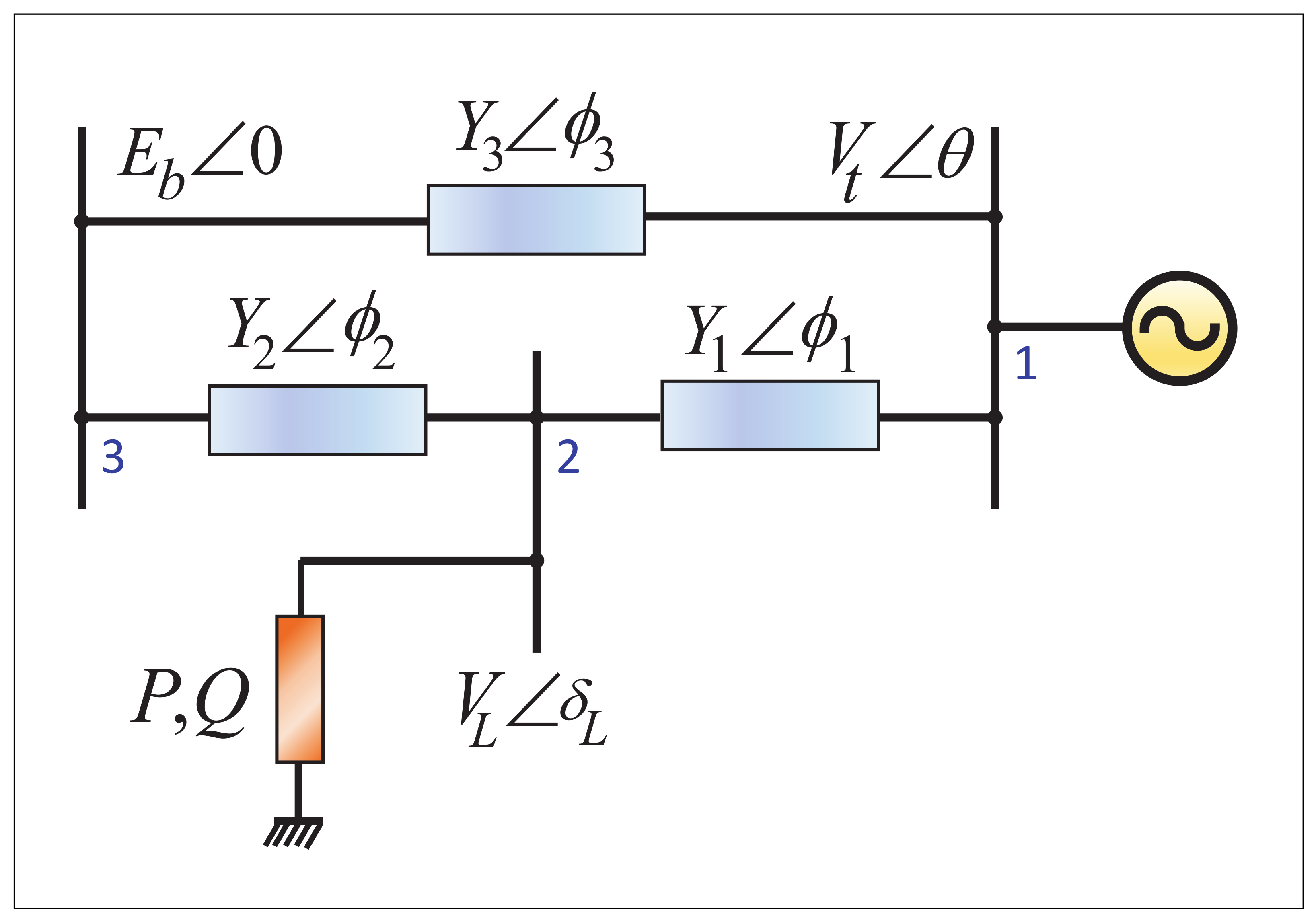
The whole controlled power system circuit diagram is shown in Figure 2. The energy storage device is located on the first bus with the generator side, while the STATCOM is connected to the second bus to support the load. To derive the mathematical model of the controlled power system [25], combine (1) and (11) yields the following system of differential Equations (12):

$$\begin{array}{c}\hfill \left\{\begin{array}{cc}{\dot{\delta }}_m\hfill & ={\omega }_B{s}_m=f_1,\hfill \\ \\ {\dot{s}}_m\hfill & {\displaystyle =\frac{1}{2H}\left(-d{s}_m+P_m-P_g-P_{\mathrm{es}}\right)=f_2}\hfill \\ \\ {\dot{P}}_{es}\hfill & {\displaystyle =-\frac{1}{T_{es}}{P}_{es}+\frac{K_{es}}{T_{es}}{u}_{es}=f_3+\frac{K_{es}}{T_{es}}{u}_{es}}\hfill \\ \\ {\dot{E}}_q^{\prime }\hfill & {\displaystyle =\frac{1}{T_{d0}^{\prime }}\left(-E_q^{\prime }+\left(x_d-x_d^{\prime }\right)I_d+E_{fd}\right)=f_4}\hfill \\ \\ {\dot{E}}_{fd}\hfill & {\displaystyle =\frac{1}{T_A}\left(-E_{fd}+K_A\left(V_{\mathrm{ref}}-V_t\right)\right)=f_5}\hfill \\ \\ {\dot{\delta }}_L\hfill & {\displaystyle =\frac{1}{q_1}\left(Q-Q_0-Q_{1d}-Q_{stat}-q_2{V}_L-\left(q_3-B_c\right)V_L^2\right)=f_6}\hfill \\ \\ {\dot{V}}_L\hfill & {\displaystyle =\frac{1}{p_2}\left[P-P_{1d}-P_0-p_3{V}_L-\frac{p_1}{q_1}\left(Q-Q_{1d}-Q_{stat}-Q_0-q_2{V}_L-\left(q_3-B_c\right)V_L^2\right)\phantom{\frac{1}{2}}\right]}\hfill \\ \\ \hfill {\dot{i}}_{stat}& {\displaystyle =-\frac{1}{T_{stat}}{i}_{stat}+\frac{K_{stat}}{T_{stat}}{u}_{stat}=f_8+\frac{K_{stat}}{T_{stat}}{u}_{stat}}\hfill \end{array}\right.\end{array}$$

(12)

where $Q_{stat}$ denotes the STATCOM reactive power provided to the load bus 2, and can be written as follows (13):

$$\begin{array}{c}\hfill \left\{\begin{array}{cc}{Q}_{stat}\hfill & =-i_{stat}{V}_L\hfill \\ f_3\hfill & {\displaystyle =-\frac{1}{T_{stat}}{P}_{es}}\hfill \\ f_8\hfill & {\displaystyle =-\frac{1}{T_{stat}}{i}_{stat}}\hfill \end{array}\right.\end{array}$$

(13)

To elaborate the controller goals, the controlled system (12) can be represented as follows (14):

$$\begin{array}{c}\hfill \left\{\begin{array}{cc}\dot{x}\hfill & =f\left(x\right)+g\left(x\right)u\hfill \\ y_1\hfill & ={\delta }_m\hfill \\ y_2\hfill & =V_L\hfill \end{array}\right.\end{array}$$

(14)

where x defines the states vector of the full controlled system (12) and $f\left(x\right)$ designates the vector of the smooth functions $f_1$ to $f_8$. $y_1$ and $y_1$ are the controlled system (12) outputs and

$$\begin{array}{c}\hfill \left\{\begin{array}{cc}u\hfill & ={\left[u_{es}{u}_{stat}\right]}^T\hfill \\ g\left(x\right)\hfill & ={\left[\begin{array}{cccccccc}0& 0& K_{es}/T_{es}& 0& 0& 0& 0& 0\\ 0& 0& 0& 0& 0& 0& 0& K_{stat}/T_{stat}\end{array}\right]}^T\hfill \end{array}\right.\end{array}$$

(15)

By defining the following transform $e_1={\delta }_m$, the three first equations of (12) can be written as:

$$\begin{array}{c}\hfill \left\{\begin{array}{cc}{\dot{e}}_1\hfill & =e_2\hfill \\ {\dot{e}}_2\hfill & =e_3\hfill \\ {\dot{e}}_3\hfill & {\displaystyle =f_9-\frac{{\omega }_B{K}_{es}}{2H{T}_{\mathrm{es}}}{u}_{\mathrm{es}}}\hfill \end{array}\right.\end{array}$$

(16)

where

$${\displaystyle f_9=-\frac{{\omega }_B}{2H}\left[d{f}_2+{\dot{E}}_q^{\prime }{I}_q+{\dot{I}}_q{E}_q^{\prime }+\left(x_d^{\prime }-x_q\right)\left(I_q{\dot{I}}_d+{\dot{I}}_q{I}_d\right)-\frac{1}{T_{es}}{P}_{es}\right]}$$

To steer the first output $y_1$ of the controlled system (14) to the zero equilibrium, the power system (16) should be stabilized to the origin. The first step in the design procedure of the synergetic control theory, is to define the macro variable which can be selected as linear combination of the state variables of system (16) as follows:

$${\psi }_1=e_3+k_2{e}_2+k_1{e}_1$$

(17)

The parameters of the macro variable ${\psi }_1$, $k_1$ and $k_2$ are selected such that the system (16) follows the required transient dynamics and the characteristic polynomial $\Delta (\lambda )={\lambda }^2+k_2\lambda +k_1$ satisfing the Hurwitz stability criteria.

To drive the system (16) dynamics evolution toward the invariant manifold ${\psi }_1=0$, the nonlinear evolution constraint defined as follows:

$$T_1{\dot{\psi }}_1+{\omega }_B\left({\psi }_1^{m_1/m_2}+{\psi }_1^{m_2/m_1}\right)=0$$

(18)

then

$$T_1{\dot{\psi }}_1=T_1({\dot{e}}_3+k_2{e}_3+k_1{e}_2)=-{\omega }_B\left({\psi }_1^{m_1/m_2}+{\psi }_1^{m_2/m_1}\right)$$

(19)

where $m_1>0$ and $m_2>0$ are design parameters selected as odd numbers and satisfy $0<m_2/m_1<1$. $T_1>0$, represents the convergence time constant that required such that the first macro-variable ${\psi }_1$ approaches the invariant attractor ${\psi }_1=0$. This design parameter selected carefully to achieve the required convergence rate. By combining (16) and (19), the required control $u_{es}$ for system (16) can be described by the following form (20):

$$\begin{array}{cc}\hfill u_{es}=& {\displaystyle \frac{2H{T}_{es}}{{\omega }_B{K}_{es}}\left[f_9+k_1{e}_2+k_2{e}_3+\frac{{\omega }_B}{T_1}\left({\psi }_1^{m_1/m_2}+{\psi }_1^{m_2/m_1}\right)\right]}\hfill \end{array}$$

(20)

Obviously, the control equation $u_{es}$ presented in (20), involves a complicated term $f_9$ which is a function of the state variables and parameters of controlled system (12). In general, complex terms render the practical application of the designed controller hard to implement [25]. Therefore, it is more realistic to employ a controller free of $f_9$. To achieve that, the control signal $u_{es}$ will be considered as a reference control for an adaptive synergetic control law $u_{es\left(ad\right)}$, that will replace the complicated control law $u_{es}$ (20). The adaptive synergetic control law can be defined as follows:

$$u_{es\left(ad\right)}=\frac{2H{T}_{es}}{{\omega }_B{K}_{es}}\left[{\widehat{k}}_1{e}_2+{\widehat{k}}_2{e}_3+\frac{{\omega }_B}{T_1}\left({\psi }_1^{m_1/m_2}+{\psi }_1^{m_2/m_1}\right)\right]$$

(21)

where the controller adaptive parameters ${\widehat{k}}_1$ and ${\widehat{k}}_2$ should be trained on-line such that the final synergetic control law $u_{es\left(ad\right)}^{*}$ matches the real complicated synergetic control $u_{es}$ (20), when the adaptive parameters ${\widehat{k}}_1$ and ${\widehat{k}}_2$ converge to the optimal values ${\widehat{k}}_1^{*}$ and ${\widehat{k}}_2^{*}$. That is:

$$u_{es\left(ad\right)}^{*}=\frac{2H{T}_{es}}{{\omega }_B{K}_{es}}\left[{\widehat{k}}_1^{*}{e}_2+{\widehat{k}}_2^{*}{e}_3+\frac{{\omega }_B}{T_1}\left({\psi }_1^{m_1/m_2}+{\psi }_1^{m_2/m_1}\right)\right]$$

(22)

To achieve this goal, the Lyapunov method will be used to derive the learning laws of the controller adaptive parameters as follows:

Theorem 1.

For the system (16), if the used control input law is given by (23), with parameters adjustment laws (24), then the macro-variable ${\psi }_1$ defined in (17) will approach the synergetic attractor ${\psi }_1=0$ and the adjusted parameters ${\widehat{k}}_1$ and ${\widehat{k}}_2$ converge to the optimal parameters ${\widehat{k}}_1^{*}$ and ${\widehat{k}}_2^{*}$, respectively.

$${\displaystyle u_{es\left(ad\right)}=\frac{2H{T}_{es}}{{\omega }_B{K}_{es}}\left[{\widehat{k}}_1{e}_2+{\widehat{k}}_2{e}_3+\frac{{\omega }_B}{T_1}\left({\psi }_1^{m_1/m_2}+{\psi }_1^{m_2/m_1}\right)\right]}$$

(23)

$$\begin{array}{c}\hfill \left\{\begin{array}{cc}{\dot{\widehat{k}}}_1\hfill & ={\omega }_B{e}_2{\psi }_1\hfill \\ {\dot{\widehat{k}}}_2\hfill & ={\omega }_B{e}_3{\psi }_1\hfill \end{array}\right.\end{array}$$

(24)

Proof. 

By substituting $u_{es\left(ad\right)}$ from (23) instead of $u_{es}$ in (16) then:

$$\begin{array}{cc}\hfill {\dot{e}}_3=& f_9-\frac{{\omega }_B{K}_{es}}{2H{T}_{es}}\frac{2H{T}_{es}}{{\omega }_B{K}_{es}}\left[{\widehat{k}}_1{e}_2+{\widehat{k}}_2{e}_3+\frac{{\omega }_B}{T_1}\left({\psi }_1^{m_1/m_2}+{\psi }_1^{m_2/m_1}\right)\right]-\frac{{\omega }_B{K}_{es}}{2H{T}_{es}}{u}_{es\left(ad\right)}\hfill \\ & +\frac{{\omega }_B{K}_{es}}{2H{T}_{es}}{u}_{es\left(ad\right)}^{*}\hfill \end{array}$$

(25)

Combining (20) and (22) with (25), system (16) be as follows:

$$\begin{array}{c}\hfill \left\{\begin{array}{cc}{\dot{e}}_1\hfill & =e_2\hfill \\ {\dot{e}}_2\hfill & =e_3\hfill \\ {\dot{e}}_3\hfill & {\displaystyle =\left({\widehat{k}}_1^{*}-{\widehat{k}}_1-k_1\right)e_2+\left({\widehat{k}}_2^{*}-{\widehat{k}}_2-k_2\right)e_3-\frac{{\omega }_B}{T_1}\left({\psi }_1^{m_1/m_2}+{\psi }_1^{m_2/m_1}\right)}\hfill \end{array}\right.\end{array}$$

(26)

Choosing a Lyapunov function as follows:

$$V_1=\frac{1}{2}{\omega }_B{\psi }_1^2+\frac{1}{2}{\left({\widehat{k}}_1-{\widehat{k}}_1^{*}\right)}^2+\frac{1}{2}{\left({\widehat{k}}_2-{\widehat{k}}_2^{*}\right)}^2$$

(27)

Then, the time derivative of $V_1$ is

$$\begin{array}{cc}\hfill {\dot{V}}_1=& {\omega }_B\psi \dot{\psi }+\left({\widehat{k}}_1-{\widehat{k}}_1^{*}\right){\dot{\widehat{k}}}_1+\left({\widehat{k}}_2-{\widehat{k}}_2^{*}\right){\dot{\widehat{k}}}_2\hfill \\ \hfill =& {\omega }_B\psi \left({\dot{e}}_3+k_1{e}_2+k_2{e}_3\right)+\left({\widehat{k}}_1-{\widehat{k}}_1^{*}\right){\dot{\widehat{k}}}_1+\left({\widehat{k}}_2-{\widehat{k}}_2^{*}\right){\dot{\widehat{k}}}_2\hfill \\ \hfill =& {\omega }_B\psi \left[\left({\widehat{k}}_1^{*}-{\widehat{k}}_1-k_1\right)e_2+\left({\widehat{k}}_2^{*}-{\widehat{k}}_2-k_2\right)e_3\right.-\frac{{\omega }_B}{T_1}\left.\left({\psi }_1^{m_1/m_2}+{\psi }_1^{m_2/m_1}\right)+k_1{e}_2+k_2{e}_3\right]\hfill \\ & +\left({\widehat{k}}_1-{\widehat{k}}_1^{*}\right){\dot{\widehat{k}}}_1+\left({\widehat{k}}_2-{\widehat{k}}_2^{*}\right){\dot{\widehat{k}}}_2\hfill \end{array}$$

(28)

Substituting (23) and (24) into (28) yields

$$\begin{array}{cc}\hfill {\dot{V}}_1=& {\omega }_B{\psi }_1\left[\left({\widehat{k}}_1^{*}-{\widehat{k}}_1-k_1\right)e_2+\left({\widehat{k}}_2^{*}-{\widehat{k}}_2-k_2\right)e_3-\frac{{\omega }_B}{T_1}{\psi }_1+k_1{e}_2+k_2{e}_3\right]\hfill \\ & +\left({\widehat{k}}_1-{\widehat{k}}_1^{*}\right){\omega }_B{e}_2{\psi }_1+\left({\widehat{k}}_2-{\widehat{k}}_2^{*}\right){\omega }_B{e}_3\left({\psi }_1^{m_1/m_2}+{\psi }_1^{m_2/m_1}\right)\hfill \\ \hfill =& -k_1{\omega }_B{e}_2\psi -k_2{\omega }_B{e}_3\psi -\frac{{\omega }_B^2}{T_1}{\psi }_1\left({\psi }_1^{m_1/m_2}+{\psi }_1^{m_2/m_1}\right)+k_1{\omega }_B{e}_2{\psi }_1+k_2{\omega }_B{e}_3{\psi }_1\hfill \end{array}$$

(29)

then

$$\begin{array}{cc}\hfill {\dot{V}}_1=& -\frac{{\omega }_B^2}{T_1}{\psi }_1\left[{\psi }_1^{m_1/m_2}+{\psi }_1^{m_2/m_1}\right]\hfill \\ \hfill =& -\frac{{\omega }_B^2}{T_1}\left[{\psi }_1^{(m_1+m_2)/m_2}+{\psi }_1^{(m_1+m_2)/m_1}\right]\hfill \end{array}$$

(30)

due to that $m_1$ and $m_2$ are odd numbers and their sum $(m_1+m_2)$ is an even then $\dot{V}\le 0$, and the system is stable. Thus the proof is completed. □

Based on the aforementioned analysis, the first control objective is achieved, where the energy storage device that is mounted to the first bus with the generator side, will damp out the chaotic oscillation as required.

The second control objective is to stabilize the load voltage $V_L$ at the rated value. For this purpose, define another non-linear transformation as $e_4=V_L-1$, so the last two equations of the controlled system (12) can be written as follows:

$$\begin{array}{c}\hfill \left\{\begin{array}{cc}{\dot{e}}_4\hfill & =e_5\hfill \\ {\dot{e}}_5\hfill & =f_{10}-\left(p_1{V}_L{K}_{stat}\right)/\left(q_1{p}_2{T}_{stat}\right)u_{stat}\hfill \end{array}\right.\end{array}$$

(31)

where

$${\displaystyle f_{10}=\frac{2}{p_2}\left(\dot{P}-\frac{p_1}{q_1}\left[\dot{Q}-\left(\frac{i_{stat}}{T_{stat}}{V}_L\right)+i_{stat}{f}_7-q_2{f}_7-2\left(q_3-B_c\right)V_L{f}_7\phantom{\frac{1}{2}}\right]-p_3{f}_7\phantom{\frac{1}{2}}\right).}$$

Obviously, when the system (31) reaches the origin, the controlled system (12) load bus voltage converges to the rated voltage $V_L=1$. Again, to use the synergetic control theory to drive the auxiliary system (31) state to achieve the required dynamics, the first step is to define a new macro variable ${\psi }_2$ which is a linear combination of the system (31) state variables as follows:

$${\psi }_2=e_5+k_3{e}_4,$$

(32)

where the stability condition in this case is to select $k_3>0$.

The synergetic macro variable ${\psi }_2$ should evolve according to the following nonlinear functional constrain:

$$T_2{\dot{\psi }}_2+\left({\psi }_2^{n_1/n_2}+{\psi }_2^{n_2/n_1}\right)=0$$

(33)

then

$$T_2{\dot{\psi }}_2=T_2({\dot{e}}_5+k_3{e}_5)=-\left({\psi }_2^{n_1/n_2}+{\psi }_2^{n_2/n_1}\right)$$

(34)

where the design parameters $n_1>0$ and $n_2>0$ are chosen odd numbers and satisfy $0<n_2/n_1<1$. $T_2>0$, represents the convergence time constant that required such that the macro variable ${\psi }_2$ attains the synergetic artificial attractor ${\psi }_2=0$. This design parameter selected carefully to satisfy the required convergence rate. By combining (31) and (34), the control law $u_{stat}$ for system (31) can be obtained as follows:

$${\displaystyle u_{stat}=\frac{q_1{p}_2{T}_{stat}}{p_1{V}_L{K}_{stat}}\left[f_{10}+k_3{e}_5+\frac{1}{T_2}\left({\psi }_2^{n_1/n_2}+{\psi }_2^{n_2/n_1}\right)\right]}$$

(35)

It is clear that, the control equation $u_{stat}$ presented in (35), involves a complicated term $f_{10}$ which is function of the state variables and parameters of controlled system (12). This complex term makes the practical application of the designed synergetic controller law difficult to implement [25], therefore it is more realistic to use a controller free of $f_{10}$. To achieve that, the control law $u_{stat}$ will be replaced by an adaptive synergetic control law $u_{stat\left(ad\right)}$, which will be equivalent to the complicated control law $u_{stat}$ (35). The adaptive synergetic control law can be defined as follows:

$${\displaystyle u_{stat\left(ad\right)}=\frac{q_1{p}_2{T}_{stat}}{p_1{V}_L{K}_{stat}}\left[{\widehat{k}}_3{e}_5+\frac{1}{T_2}\left({\psi }_2^{n_1/n_2}+{\psi }_2^{n_2/n_1}\right)\right]}$$

(36)

where the adaptive parameters ${\widehat{k}}_3$ should be adjusted on-line such that the final synergetic control law $u_{stat\left(ad\right)}^{*}$ matches the real complicated synergetic control $u_{stat}$ (35), as similar to the previous reasoning.

$$\begin{array}{cc}\hfill u_{stat\left(ad\right)}^{*}& =\frac{q_1{p}_2{T}_{stat}}{p_1{V}_L{K}_{stat}}\left[{\widehat{k}}_3^{*}{e}_5+\frac{1}{T_2}\left({\psi }_2^{n_1/n_2}+{\psi }_2^{n_2/n_1}\right)\right]=u_{stat}\hfill \end{array}$$

(37)

Theorem 2.

For the system (31), if the used control input law is given by (38), with parameter adjustment law (39), then the macro-variable ${\psi }_2$ defined in (32) will approach the synergetic attractor ${\psi }_2=0$ and the adjusted parameter ${\widehat{k}}_3$ converges to the optimal value ${\widehat{k}}_3^{*}$.

$$u_{stat\left(ad\right)}=\frac{q_1{p}_2{T}_{stat}}{p_1{V}_L{K}_{stat}}\left[{\widehat{k}}_3{e}_5+\frac{1}{T_2}\left({\psi }_2^{n_1/n_2}+{\psi }_2^{n_2/n_1}\right)\right]$$

(38)

$${\dot{\widehat{k}}}_3=e_5{\psi }_2$$

(39)

Proof. 

By substituting $u_{stat\left(ad\right)}$ from (38) instead of $u_{stat}$ in (31) then:

$$\begin{array}{cc}\hfill {\dot{e}}_5=& f_{10}-\left({\widehat{k}}_3{e}_5+\frac{1}{T_2}\left({\psi }_2^{n_1/n_2}+{\psi }_2^{n_2/n_1}\right)\right)-\frac{q_1{p}_2{T}_{stat}}{p_1{V}_L{K}_{stat}}{u}_{stat}+\frac{q_1{p}_2{T}_{stat}}{p_1{V}_L{K}_{stat}}{u}_{stat\left(ad\right)}^{*}\hfill \end{array}$$

(40)

Using (35), (37) and (40), then the controlled system (31) can be written as follows:

$$\begin{array}{c}\hfill \left\{\begin{array}{cc}{\dot{e}}_4\hfill & =e_5\hfill \\ {\dot{e}}_5\hfill & =\left({\widehat{k}}_3^{*}-{\widehat{k}}_3-k_3\right)e_5-\frac{1}{T_2}\left({\psi }_2^{n_1/n_2}+{\psi }_2^{n_2/n_1}\right)\hfill \end{array}\right.\end{array}$$

(41)

Choosing the Lyapunov candidate function as:

$$V_2=\frac{1}{2}{\psi }_2^2+\frac{1}{2}{\left({\widehat{k}}_3-{\widehat{k}}_3^{*}\right)}^2$$

(42)

Then, the time derivative of $V_2$:

$$\begin{array}{cc}\hfill {\dot{V}}_2& ={\dot{\psi }}_2{\psi }_2+\left({\widehat{k}}_3-{\widehat{k}}_3^{*}\right){\dot{\widehat{k}}}_3\hfill \\ \hfill & ={\psi }_2\left({\dot{e}}_5+k_3{e}_5\right)+\left({\widehat{k}}_3-{\widehat{k}}_3^{*}\right){\dot{\widehat{k}}}_3\hfill \end{array}$$

(43)

By combining (38), (39) and (41) with (43), obtain:

$$\begin{array}{cc}\hfill {\dot{V}}_2& ={\psi }_2\left[\left({\widehat{k}}_3^{*}-{\widehat{k}}_3-k_3\right)e_5-\frac{1}{T_2}\left({\psi }_2^{n_1/n_2}+{\psi }_2^{n_2/n_1}\right)k_3{e}_5\phantom{\frac{1}{2}}\right]+\left({\widehat{k}}_3-{\widehat{k}}_3^{*}\right)e_5{\psi }_2\hfill \\ \hfill & =-k_3{e}_5{\psi }_2-\frac{1}{T_2}{\psi }_2\left({\psi }_2^{n_1/n_2}+{\psi }_2^{n_2/n_1}\right)+k_3{e}_5{\psi }_2\hfill \\ \hfill & =-\frac{1}{T_2}\left({\psi }_2^{(n_1+n_2)/n_2}+{\psi }_2^{(n_1+n_2)/n_1}\right),\hfill \end{array}$$

(44)

since $n_1$ and $n_2$ are odd numbers then their sum $(n_1+n_2)$ is an even and ${\dot{V}}_2\le 0$, so the system is stable.

Therefore, the proof is completed. □

According to that, the second objective of the designed control algorithm is achieved, where the STATCOM compensator will drive ${\psi }_2$ toward the artificial attractor ${\psi }_2=0$, therefore the system (31) reaches the origin equilibrium and restores the load bus voltage $V_L$ to its rated value.

5. Simulation Results

The parameters values of the three-bus power system are adopted as in [25]. All the parameters values are listed in Appendix B. The system (1) initial values are (${\delta }_m\left(0\right)$, $s_m\left(0\right)$, $E_q^{{}^{\prime }}\left(0\right)$, $E_{fd}\left(0\right)$, ${\delta }_L\left(0\right)$, $V_L\left(0\right)$) = ($1.3331$, 0, $1.0312$, $2.9982$, $0.3858$, $0.9845$). The power system (1) exhibits chaotic oscillation, the chaotic nature of the system is characterized as in Figure 3 and Figure 4. As can be seen from Figure 3a, chaotic signature of the power system is illustrated by the trajectory evolution in the 3D phase plane which reflects the strange nature of the orbits. The power spectral density for 100 $\left(s\right)$ time waveforms and sampling period of 0.005 $\left(s\right)$ and the bicoherence diagram for the power system (1) are given in Figure 3b. The bicoherence is significantly nonzero, and nonconstant, indicating a strong nonlinear relationship between the power system states, and the broadened power spectrum are both signatures of the chaos phenomenon. 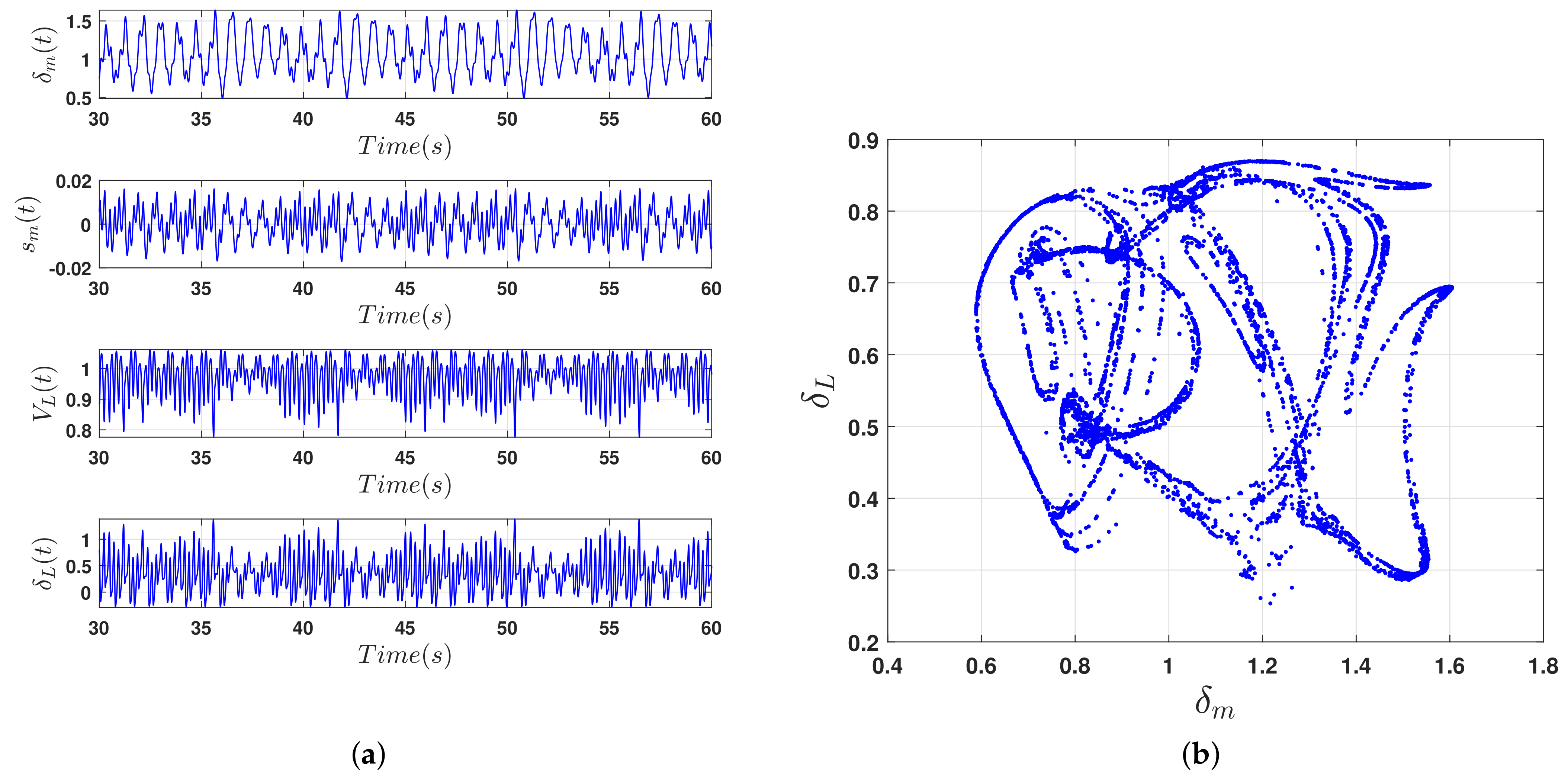Figure 4a shows that the time waveforms of state variables (${\delta }_m\left(t\right)$, $s_m\left(t\right)$, $V_L\left(t\right)$) are aperiodic with irregular oscillatory behaviors, therefore it is an impossible to predict their trajectories evolution after a long period of time. Poincaré map is plotted in Figure 4b projected in the (${\delta }_m\left(t\right)$, ${\delta }_L$) plane, which clearly reveals the chaotic dynamics of the power system. Further, employing Wolf’s algorithm [45], the largest Lyapunov exponent found equals to 0.4360. The positive Lyapunov exponent indicates the existence of chaotic attractor. Chaotic oscillation has been considered as one of the main routes that will lead power system to voltage collapse. Therefore, an immediate control action needs to be activated to suppress chaos and restore the normal operation.

The controller parameters should be selected to satisfy the following constraints derived in stability analysis. The roots of the characteristic’s equation of the first manifold (17) will be located at ${\lambda }_{1,2}=-5$, therefore the characteristic equation will be ${\lambda }^2+10\lambda +25=0$, from that it can be concluded that $k_1=25$ and $k_2=10$. For the second manifold (32) the root of its characteristic equation will be located at $\lambda =-10$, then its characteristic equation will be $\lambda +10=0$, therefore $k_3=10$. Noting that the largest values for $\left|{\lambda }_{1,2,3}\right|$ the faster motion will be achieved on the synergetic attractor because the roots will be far from the imaginary axis in the complex plane. Regarding the selection of $m_1$, $m_2$, $n_1$ and $n_2$ they should be positive odd numbers and meet the conditions $0<m_2/m_1<1$ and $0<n_2/n_1<1$ as stated in Lemma 1. The strength of the nonlinear manifold will be more obvious when these numbers are chosen somewhat large, so they are considered equal to $m_1=9$, $m_2=7$, $n_1=9$, $n_2=7$. $T_1$ and $T_2$ which are designer-chosen determine the rate of convergence to the synergetic manifold and can be made arbitrary small considering only eventual control constraint. Hence $T_1$ and $T_2$ can arbitrarily be chosen equal to $0.05$. The initial values of the adaptive parameters can be randomly selected as ${\widehat{k}}_1\left(0\right)=1$, ${\widehat{k}}_2\left(0\right)=2$ and ${\widehat{k}}_3\left(0\right)=3$. All the aforementioned controller parameters can be tuned using different optimization algorithms such as evolutionary algorithm (EA), genetic algorithm (GA), particle swarm optimization (PSO), bats algorithm (BA), and many other methods [46,47,48], or can be simply selected by the trial-and-error method under the stated conditions. On the other hand, the selection of $K_{es}$, $T_{es}$, $K_{stat}$, $T_{stat}$ given in the same framework as in [25,35,43]. These parameters are only used to illustrate the effectiveness of the designed control algorithm. In practical applications, these values can be selected according to the actual operating conditions of the system. Without loss of generality, the design parameters can be selected as but not limited to $K_{es}=10$, $T_{es}=0.1$, $K_{stat}=1$, $T_{stat}=1$.

The control objective is to suppress chaos in the power system and stabilize the power system to its desired operating point ${\delta }_{md}=0$, $s_{md}=0$ and $V_{Ld}=1$. Three simulation scenarios are conducted to examine the proposed controller performance in suppressing chaos in the power system and managing STATCOM and the energy storage device through an adaptive synergetic control algorithm.

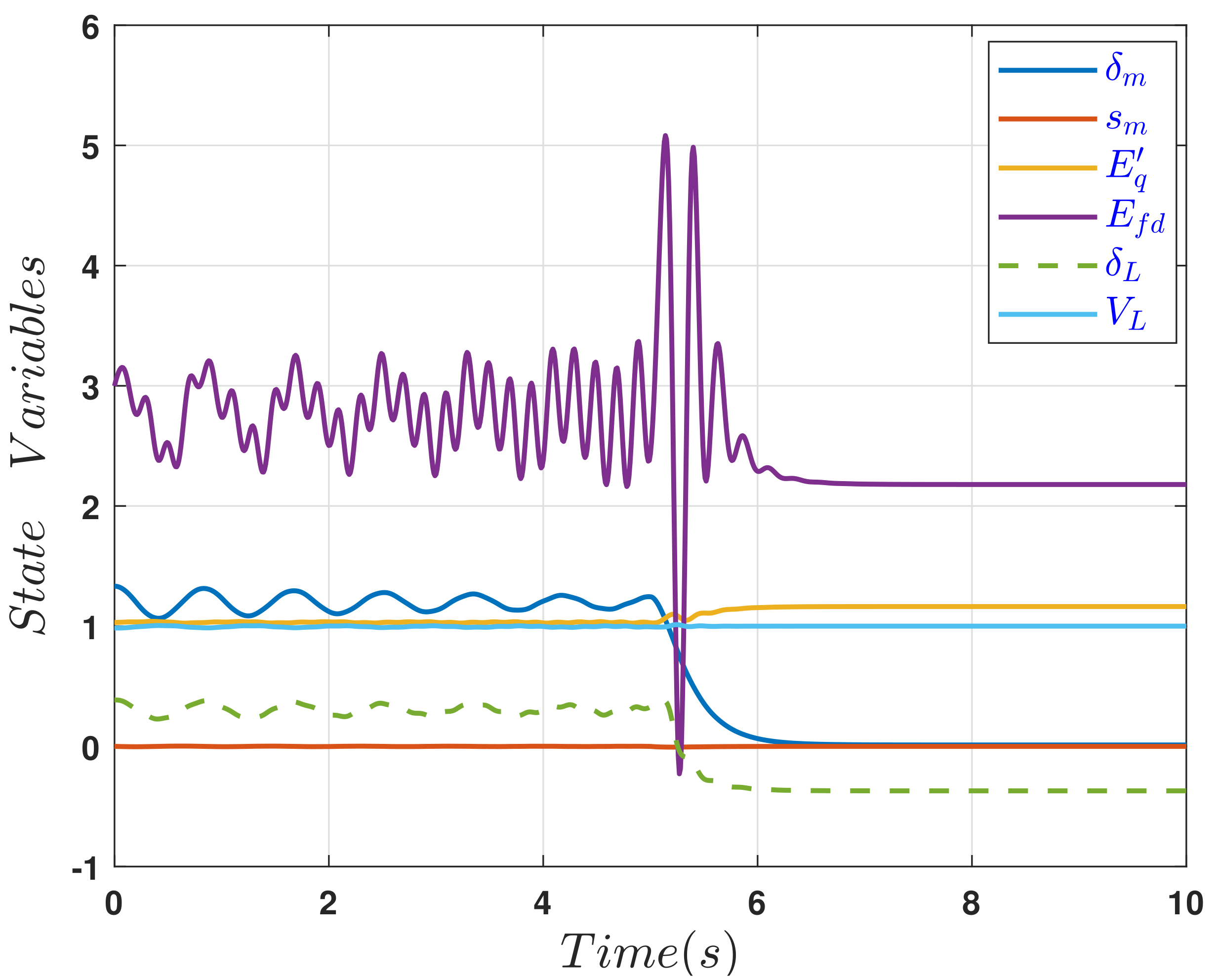
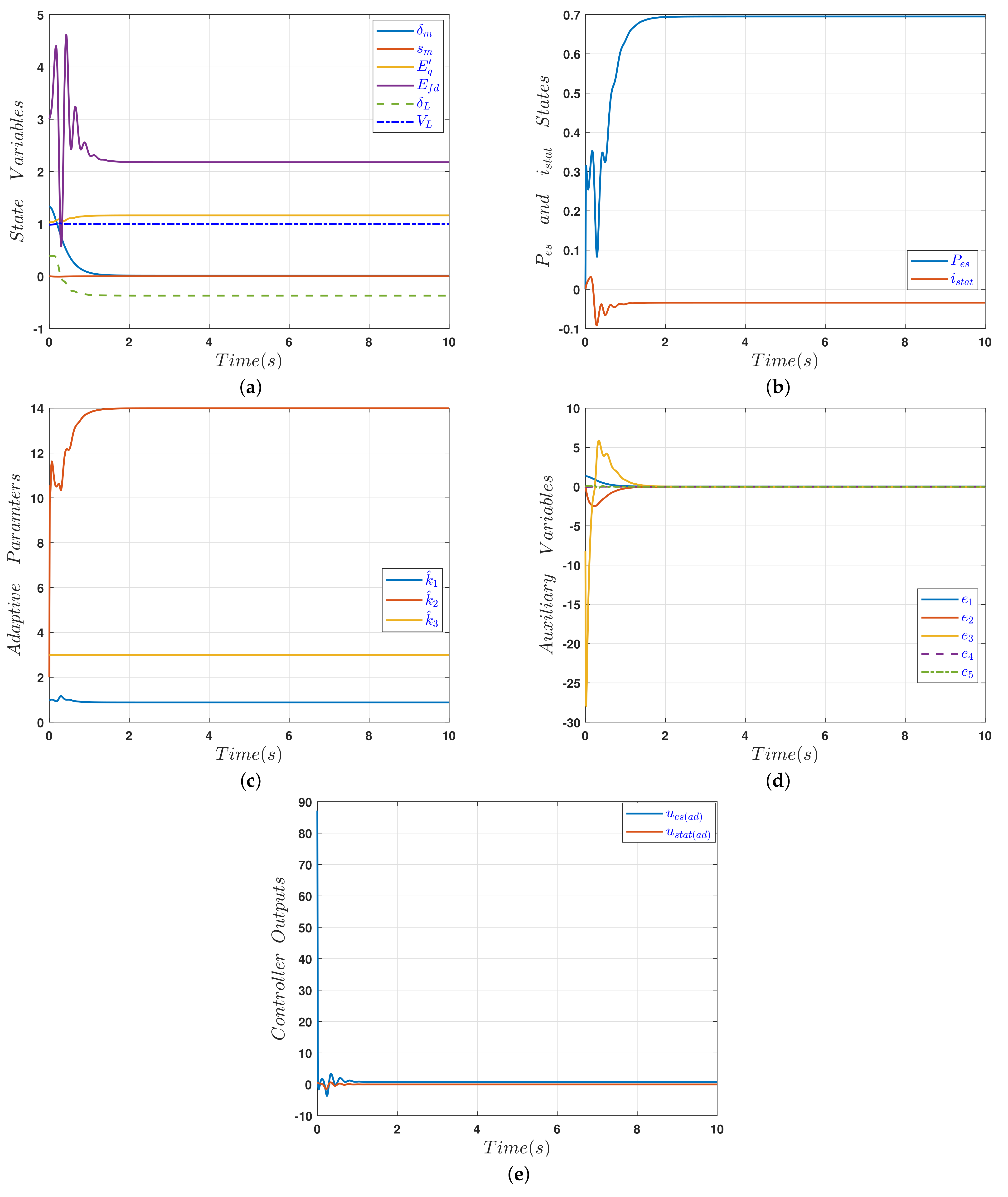
In the first scenario, the controller has been activated from the beginning of simulation time to stabilize the chaotic power system dynamics. The results of the first scenario are given in Figure 5. The time waveforms of state variables of the three-bus chaotic power system with the proposed controller are presented in Figure 5a. It clearly demonstrates the chaotic oscillation has been suppressed completely and the controller achieved the control objectives. The results verify the effectiveness of the designed controller scheme.

The STATCOM compensator and the energy storage device states are presented in Figure 5b. The controller adaptive parameters converge to steady-state values in finite time as shown in the parameters time courses that are given in Figure 5c. Figure 5d shows the system auxiliary variables time-domain waveforms heading toward the origin. The waveforms reveal that the controller can achieve as fast a convergence rate as required. The controller output is presented in Figure 5e and it is chattering free and smooth signals.

In the second scenario, the controller is deactivated at the outset of simulation, therefore, the power system state variables move chaotically with time, until when the controller is switched on at an arbitrary time $t=5\left(s\right)$ the state variables are controlled, the erratic oscillation is damped out and the system dynamics converge to the desired states as shown in Figure 6.

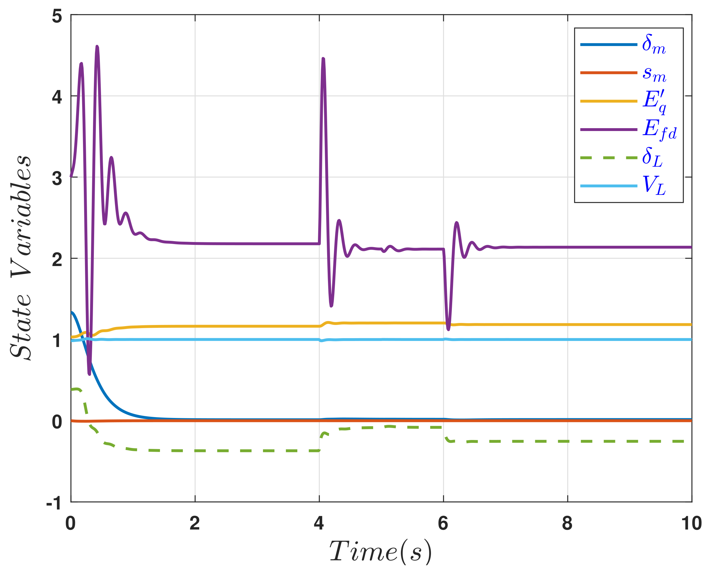
In the third scenario, power fluctuation due to load variation is applied to verify the robustness of the designed control algorithm. The disturbance can be achieved in the power system (1), by considering the parameters $P_{1d}$ that represents the load active power and $Q_{1d}$ which defines the load reactive power, where changing these parameters, presents mismatched-disturbances to the system (12) [25]. By setting the active power disturbance as $\Delta P_{1\left(ds\right)}=-0.2·\mu (t-5)+0.3·\mu (t-6)$ [W], and the fluctuation in reactive power as $\Delta Q_{1\left(ds\right)}=0.2·\mu (t-4)-0.1·\mu (t-6)$ [var] where $\mu \left(t\right)$ denotes the unit step function in this context. The simulation result of this case is shown in Figure 7. Figure 7 shows the time waveform of the controlled power system (12) states. The results in Figure 7 reveal that the suggested controller is robust against the disturbances and successfully able to suppress the chaotic oscillation effectively and maintain all state variables of the controlled system at the objective state as required.

6. Conclusions

The intent of this paper is to investigate the problem of suppressing chaotic oscillation in a three-bus power system. The chaotic power system is modeled using a six nonlinear differential equations system. The system dynamics exhibit a critical chaotic oscillation at specific system parameter values that affect the power system bus voltage stability. Chaos phenomena in the power system can lead to system collapse, which highly affects the quality of commercial power service. Therefore, an adaptive synergetic control algorithm with the help of STATCOM and energy storage devices is designed to realize the controller. The adaptive algorithm is designed, based on the Lyapunov approach, to overcome the system complexity and reduce the controller structure. The simulation results provided for different scenarios, indicated that the suggested control scheme effectively damped out chaos oscillation in the power system, achieving an appropriate transient response with a robust disturbance rejection feature.