Article

MSAM: Modular Statistical Analytical Model for MAC and Queuing Latency of VLC Networks under ICS Conditions

1
Department of Computer Engineering, College of Computer and Information Technology, Taif University, P.O. Box. 11099, Taif 21994, Saudi Arabia
2
Department of Computer Engineering, College of Computer and Information Systems, Umm Al-Qura University, Makkah 21955, Saudi Arabia
*
Author to whom correspondence should be addressed.
Electronics 2021, 10(12), 1371; https://doi.org/10.3390/electronics10121371
Submission received: 3 May 2021 / Revised: 30 May 2021 / Accepted: 31 May 2021 / Published: 8 June 2021
(This article belongs to the Section Microwave and Wireless Communications)

Abstract

:
Visible Light Communication (VLC) offers distinctive advantages over conventional radio frequency; wide unlicensed spectrum, resistance to electrometric interference and low susceptibility to security risks, are few to name. Excitingly, VLC becomes a cornerstone in several communication systems such as light fidelity, optical camera communication and the Internet of Radio Light. Most of these networks adopt the Carrier Sensing Multiple Access-Collision Avoidance (CSMA-CA) of IEEE 802.15.7, the official standard for the VLC, as a Medium Access Control (MAC) protocol. Motivated by the crucial roles of MAC in shaping the performance of the VLC and the wide variety of operational conditions demanded by the enormous applications, this paper proposes a Modular Statistical Analytical Model (MSAM). The fundamental approach of MSAM is to segregate the interacting stochastic processes imposed by the CSMA-CA protocol into a set of its elementary subprocesses. The MSAM then synthesises these processes in such a way that quantifies their mutual dependency without making a strict assumption on their characteristics; thus, different operational conditions can be assessed without a need to reconstruct the model. Besides, MSAM employs the radiometry and photometry of VLC to derive mathematical expressions describing the hidden and exposed nodes from which the Imperfect Carrier Sensing (ICS) conditions are defined. The MSAM exploits statistical and queuing theorems to model a VLC as a network of G/G/1 queues from which several probability distributions, characterising the operations of VLC from different perspectives, are derived. Inter-departure, queuing, service time and successful service time are the main distributions in conjunction with throughput, total delay, probability of exposed and hidden node collisions, which are the main outputs of MSAM. Validation for the integrity of the MSAM under different scenarios is carried out by conducting a head-to-head comparison between its results and simulation outcomes.

1. Introduction

Visible Light Communication (VLC) is a sort of wireless communication technology that utilises those segments of the electromagnetic spectrum falling within the human visual range [1] as media and optoelectronics devices as communication parties. Employing the visible light spectrum offers multiple advantages, including promoting wireless communication with more than 360 THz of unlicensed bandwidth, which is 10,000 times wider than the entire (RF) band [2]. This makes VLC one of the cost-effective and robust candidates to resolve the spectrum congestion of RF. Moreover, utilising optoelectronics devices in VLC means that the signals emitted and received by VLC (i.e., light beams) are immune to RF interference, which in turn facilitates using wireless technology in those areas where RF is restricted, e.g., medical operating theatres, chemical plants and aeroplanes [3]. Moreover, this immunity allows using VLC as complementary to other communication technologies such as power line communication or even RF. Another appealing advantage of the VLC is due to the fact that the light beams used in VLC are confined spatially within a bounded chamber. This hinders their penetration and, in turn, makes VLC secure against several types of attacks that can occur to RF systems [4].
Stimulated by these advantages, the Institute of Electrical and Electronics Engineers (IEEE), in 2011, released IEEE 802.15.7 standard [5] to specify the physical and Medium Access Control (MAC) sublayers of VLC. This standard coincided with the rapid development of the optoelectronics industry, which resulted in the massive proliferation of VLC-based networks. Light Fidelity (LiFi) [6], Lighting Emitted Diode (LED) to LED communications [7], optical camera communications [8] and smart toys network [9] are a few to name. Furthermore, the IEEE 802.15.7 standard facilitates the integration of VLC with other pertinent and forthcoming technologies to devise novel approaches, e.g., 5G Infrastructure Public-Private Partnership and beyond [10], intelligent transportation system [11] and Internet of Radio Light [12].
IEEE 802.15.7 standard defines different data rates, modulation schemes, network topologies and so on, for both indoor and outdoor environments to meet the different operational conditions required by massive VLC applications. However, this standard defines the Carrier Sense Multiple Access-Collision Avoidance (CSMA-CA) as the essential channel regulation scheme [5]. CSMA-CA is a contention-based MAC protocol in which a node, before commencing a transmission, conducts a scan over its sensing range (i.e., carrier sensing) to check if another transmission is occurring. If so, the node defers its transmission for a random period and then conducts sensing again; otherwise, it commences transmission. Hence, packets can be exchanged without being susceptible to a high level of collision probabilities as in the ALOHA scheme [13] (ALOHA allows a node, whenever it has a packet, to commence transmission regardless of the channel condition). Another main advantage of the CSMA-CA protocol is that it is a decentralised scheme; hence, there is no need to make reservations before transmissions, which in turn imposes no overhead on the VLC networks, making it suitable for delay-sensitive applications.
However, one of the main flaws of the CSMA-CA is the so-called Imperfect Carrier Sensing (ICS) [14,15,16,17], which characterises the situations under which the carrier sensing mechanism is insufficient to limit packet collisions, i.e., the exposed node problem and hidden node problem. ICS has detrimental effects on the performance of a wireless network operating CSMA/CA, as it can lessen the throughput, enlargement packet’s queuing and medium access delay, as well as degrading channel utilisation. Interestingly, these effects become more detrimental in VLC due to the narrow sensing range of optoelectronic devices and the directionality of the light beams [16,17]. Evaluating the effects of the ICS on the performance of IEEE 802.15.7 CSMA-CA is a challenge as ICS results from the interaction amongst several stochastic processes; specifically, the stochastic processes that generate packets, manage durations between two consecutive CSMA-CA channel assessments and outline the directivity of light beams. Several works have been devoted to overcoming this challenge by employing one or more simplification assumptions, such as a transmitter that can see all ongoing transmissions from other nodes [18,19,20,21,22], or when the traffic generated by a node is set in accordance with the channel status, as proposed in [16,17].
Motivated by the importance of developing a rigorous assessment tool for the IEEE 802.15.7 CSMA-CA protocol considering general cases, this paper proposes a new model dubbed the Modular Statistical Analytical Model (MSAM). The underlying approach of MSAM is to segregate the interacting stochastic process into a set of elementary subprocesses and spell out their behaviour over the complete probability distribution. By this means, MSAM can assess the performance of the IEEE 802.15.7 CSMA-CA protocol under a wide variety of operational conditions without the need to rebuild a dedicated model for each condition. The main contributions of this work can be summarised as follows:
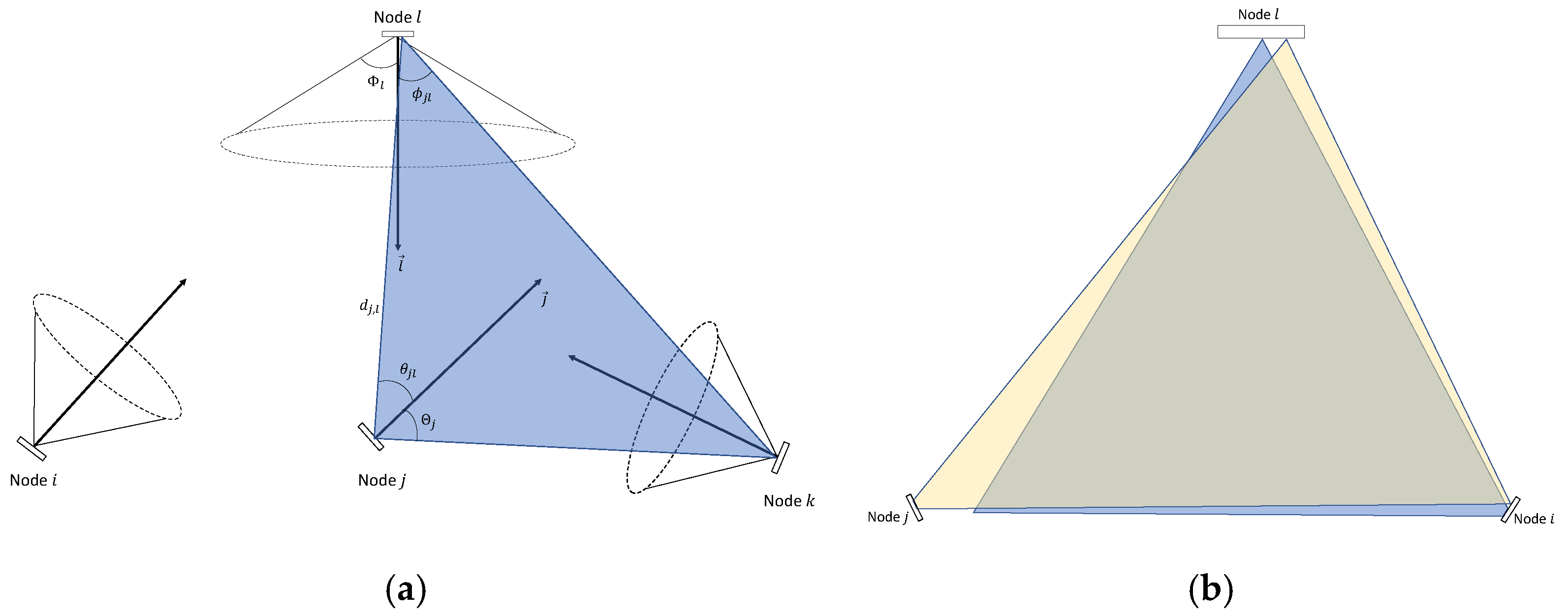
  • Develop a novel approach to model a VLC network operating the IEEE 802.15.7 CSM-CA protocol as a network of mutually dependent queues whose inter-arrival and service time distributions are of the general form, i.e., a network of G/G/1 queues. Subsequently, apply the principles of the tagged user analysis [23,24,25,26] to define the key assumptions under which dependency is decoupled, considering the distinct contention behaviour used by each node to access the shared channel. Moreover, this study employs the radiometry and photometry characteristics of the VLC [2] and set theory [27] to develop mathematical expressions describing the hidden and exposed node from a perspective of an arbitrary node within the network.
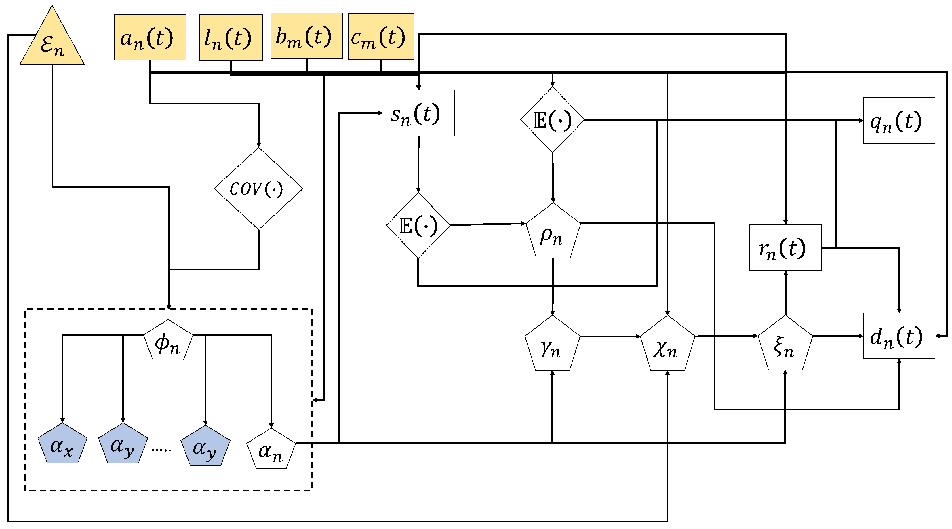
  • Derive the service time distribution that quantifies the CSMA-CA operations based on near-real assumptions. Subsequently, utilise some of the statistical and queuing theorems in conjunction with the modularity approach of MSAM to generate several distributions signifying the network’s operations from different aspects, i.e., the probability distributions of the time required to service successful packets, packet’s inter-departure distribution and the distribution of queueing delay. Besides the derivation of these distributions, MSAM also offers several metrics to measure the performance of MAC protocol, including the probability of exposed and hidden node collisions, probability of dropping packet due to exceeding the maximum number of busy channel assessments, network throughput, packets’ average delay and jitter.
  • Provide extensive assessment for the integrity of MSAM by comparing its results with the simulation outcomes, considering several scenarios, e.g., heterogeneous traffic patterns, various network densities and the different number of hidden and exposed nodes. The results of these assessments demonstrate the ability of MSAM to predict the performance of the IEEE 802.15.7 CSMA-CA protocol precisely.
The remainder of this paper is organised as follows: Section 2 provides the relevant materials, including an overview of the IEEE 802.15.7 CSMA-CA mechanism in Section 2.1, discussion of the Imperfect Channel Sensing in Section 2.2 and exploration of related works in Section 2.3. Section 3 presents the methods of this work in two Subsections: Section 3.1 introduces the assumptions underpinning MSAM, and Section 3.2 derives the MSAM. The results of this work and discussion are given in Section 4 and Section 5, respectively. Finally, Section 6 concludes this work.

2. Materials

The IEEE 802.15.7 [5] is the first international standard specifying the physical and Medium Access Control (MAC) protocols of the short-range VLC networks. This standard defines several physical types with different data rates to cover various indoor and outdoor scenarios. Furthermore, the IEEE 802.15.7 standard features several network topologies that can be operated using either beacon or beacon-less modes. The former requires that all nodes within the same VLC network be synchronised, whereas the latter allows nodes with different timing drifts to communicate freely. Besides, the IEEE 802.15.7 standard defines two MAC schemes: contention-less and Carrier Sense Multiple Access-Collision Avoidance (CSMA-CA). The contention-less scheme is used in the beacon mode to allow those nodes that wish to send their packets in the next synchronisation cycle to make a prior reservation. The contention-less approach is adopted in this standard to address the requirements of some applications that need periodic reporting. Thus, the standard defines the contention-less scheme as optional and restricts its usage over a certain number of slots within a synchronisation cycle. Conversely, the standard allows using the CSMA-CA protocol over both the beacon and beacon-less modes without any constraints.
For the sake of generality, this study considers a single-hop network operating beacon-less mode with the IEEE 802.15.7 CSMA-CA protocol; an overview of this protocol is given in Section 2.1, and the ICS conditions of the VLC are demystified in Section 2.2. The related work conducted to analyse the performance of VLC is explored in Section 2.3.

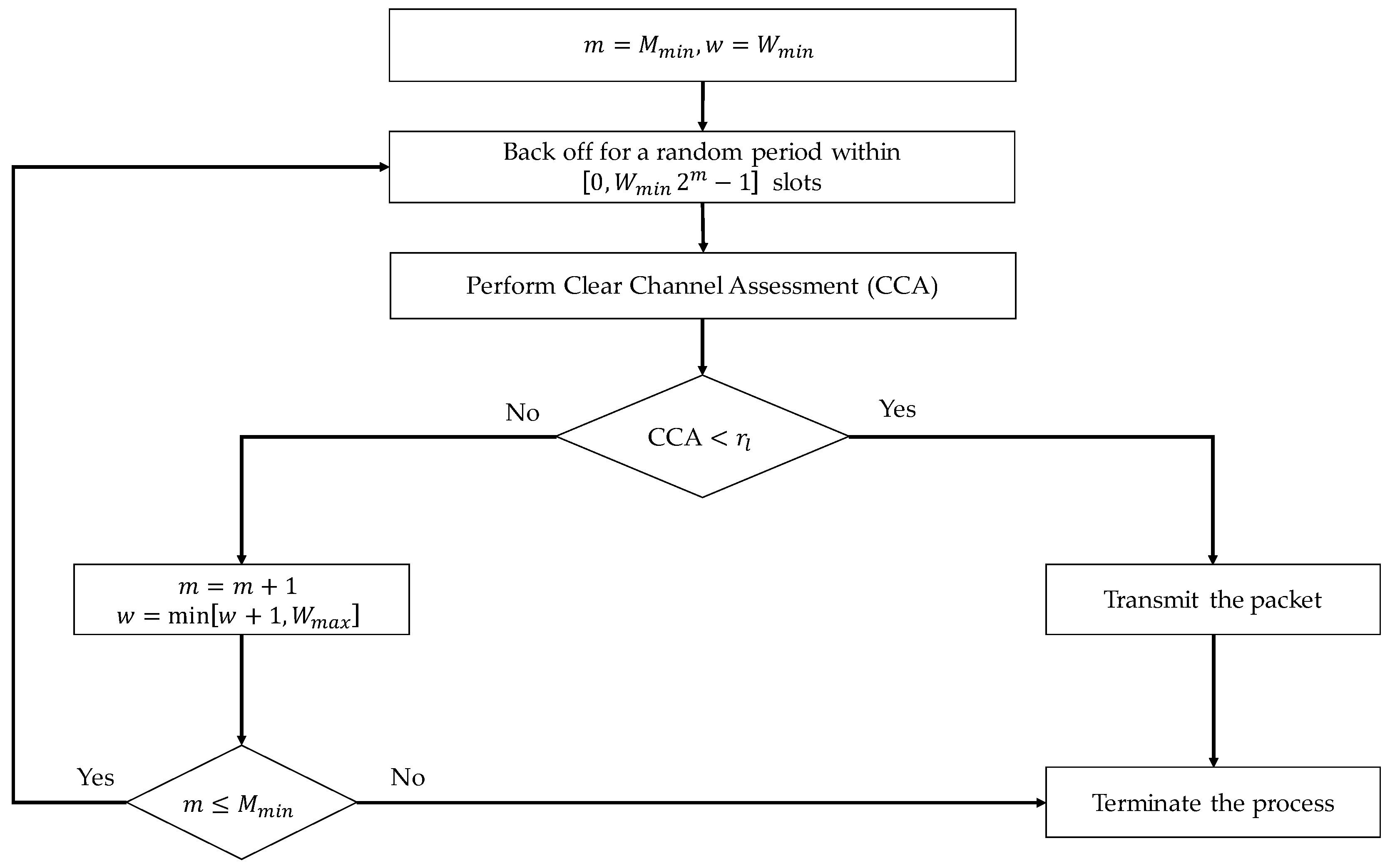
2.1. Overview of the IEEE 802.1.7 CSMA-CA Protocol

According to the IEEE 802.115.7 standard [5], an optoelectronic node, also referred to here as Visible Light Node (VLN), starts the CSMA-CA mechanism by setting the number of back-off ( m ) and back-off window ( w ) to their minimum values, which are M m i n   = 0 and W m i n   = 3 , respectively. Afterwards, a VLN backs off for a random number of slots generated according to a uniform distribution whose support is [ 0 ,   W m i n   2 m 1 ] ; where the slot is the smallest timing unit used to manage the CSMA-CA activities, its value being 60 optical clocks [5]. Upon elapsing of the back-off period, a node performs a Clear Channel Assessment (CCA) for one slot to ensure that the channel is idle (i.e., the energy of the channel is less than the receiver’s sensitivity, r l ); if so, then a node commences transmission. Otherwise, a node increments the values of m and w and backs off for another random period; at the end of which, the CCA is conducted again. Such an operation is repeated until a node either finds an idle channel and transmits its packet or drops it due to exceeding the maximum number of busy channel assessments m M m a x . Figure 1 illustrates the flowchart of this protocol.

2.2. Imperfect Channel Sensing (ICS)

In this study, Imperfect Channel Sensing (ICS) refers to cases in which the carrier sensing mechanism fails to prevent collisions amongst the packets sent towards the same receiver. Two cases are defined under ICS: exposed node collision and hidden node collision. For the sake of illustration, Figure 2 shows a conceptual diagram of a VLC network comprising four nodes: i , j , k and l .
In Figure 2a, it is assumed that node j is commencing a transmission towards node l , while both i and k are performing a clear channel assessment to check if the channel is ready to accommodate their potential transmissions towards l . As it can be seen, the light beams emitted by j cannot be sensed by node i ; hence, i shall assess idle channel and consequently commence transmission resulting in a collision at the receiver (node l ). Since transmission of j is not seen by node i , this type of collision is dubbed as a hidden node collision.
On the other hand, the exposed node collision occurs when two or more nodes are within the carrier sensing range of each other, and hence a transmission from a node can be sensed by the other. Figure 2b shows a simple case in which the light beams of node i can be seen by node j and vice versa. Hence, the exposed node collision occurs when both i and j sense the channel simultaneously as idle and then commence their transmission towards l concurrently, resulting in head-to-head overlapping between packets.
It is important to note that most of the analytical works reported in the literature assume that all nodes of a VLC network are within the carrier sensing range of each other, which limits the ICS to exposed node collisions only. While this assumption has been adopted to reduce the mathematical intractability, the simulation-based assessments of hidden node collisions reported in [16] demonstrate their significant impacts. This work aims to develop a robust analytical model that can account for general ICS cases. Here, we adopt the set theory [27] in conjunction with radiometry of VLC [2] to derive mathematical expressions quantifying the collections of nodes that constitute hidden/exposed nodes from a perspective of an arbitrary node. This expression will be employed in deriving the collision probabilities and probability generating function of the time required to service a successful packet, in Section 3.
Let us assume that S is a set comprising all the Visible Light Nodes (VLNs) within a VLC network; for an arbitrary two VLNs within this networks, e.g., j , l S , the DC channel gain of transmission from j towards the l , denoted by H j , l ( 0 ) can be given as [2]:
H j , l ( 0 ) = { A l ( m j + 1 ) 2 π d j , l 2 cos m ( θ j l ) T ( ϕ j l ) G ( ϕ j l ) cos ( ϕ j l ) , 0 < ϕ j l Φ j 0 , otherwise
where A j is the physical areas of the photodiode detector of the receiver; d j , l is the distance between j and l ; m j is order of Lambertian emission, which is computed as ln ( 2 ) ln ( cos ( Θ j ) ) where Θ j is the transmitter semi-angle at half power; θ j l is the angle of the radiance of the light beam emitted from j to the l measured with respect to the normal of the plan of j , which is denoted by j ; ϕ j l is the angle of incidence of the light beam emitted from j to l measured with respect to the normal of the plan of l , which is denoted by l . T ( ϕ j l ) is the signal transmission coefficient of the optical filter of j due to the transmission to node l , and G ( ϕ j l ) is the receiver optical concentrator gain of node j due to the transmission to node l . Φ l is the field of view of the receiver l . Figure 2a shows these symbols and parameters.
Let P j be the transmission power of j , then the power received by l due to P j can be computed as:
P j , l = H j , l ( 0 ) · P j
From the perspective of node j , an element of S other than l , i.e., x { S / { j , l } } constitutes an exposed node, if the power received to it due to transmission of j is greater than or equal to its receiver sensitivity. Let j be a set that comprises all exposed nodes of j and r x be the receiver sensitivity of node x , then:
j = { x { S / { j , l } } : P j , l r x }
Consequently, the set of hidden nodes of j can be defined as the complement of j , i.e., j ¯ = { S / j } .
Although this derivation considers the line-of-sight propagation scenario, other scenarios can be adopted readily just by replacing Equation (2) with the corresponding channel gain. However, the key reason for adopting this channel model is that the main thrust of this work is to assess the performance of the CSMA-CA protocol considering a general case; thus, adopting a particular channel model can limit this generality due to the wide variety of VLC applications and their corresponding channel models. Another cogent reason for adopting this simple channel model here is that adopting other channel models can add significant randomness to the performance metrics, which can hinder understanding the intrinsic behaviour of CSMA-CA. It is also worth noting that most of the related works [16,18,19,20,21,22] employ the same channel model justified by the results of several studies investigating the channel model of indoor VLC [28,29,30], which conclude the tiny effects of NLOS.

2.3. Related Works

Evaluating the performance of the MAC protocols of wireless networks is a longstanding practice that has been conducted by enormous works using different approaches and techniques. Notwithstanding, a few of these works have been devoted to the VLC networks owing to their special characteristics and the newness of their protocols. Here, we attempt to explore the pertinent works, highlight their underlying assumptions and main contributions as well as pointing out their limitations with the aim to underline the motivations of this work.
Using simulation platforms to investigate the IEEE 802.15.7 CSMA-CA protocol’s performance constitutes one of the mainstream themes that appeared in several works. For instance, [18] evaluates the effects of the beacon mode parameters on the performance of the network, specifically, to assess the frequency and the length of the control frames broadcasted by the coordinator to define the synchronisation cycles of the VLNs. This work considers a single-hop network operating over an idle channel condition and saturation traffic pattern, i.e., the pattern in which a VLN always has a packet ready to be sent. During the simulation session, this work assumes that the CSMA-CA protocol is the sole media regulation schema and that all other nodes can see the transmission of a node. However, it replaces the default binary exponential back-off ratified in the standard by a new scheme in which the back-off windows of collided nodes are increased multiplicatively based on the number of collisions. Several results reported in this work demonstrate that lessening the frequency of the control frame can significantly improve the throughput of the network. However, the over-simplification assumptions employed in this work in terms of the new back-off scheme, saturation traffic pattern, and ignoring ICS conditions limit its results’ generalisation.
The authors of [16] introduce a simulation-based study to investigate the performance of the IEEE 802.15.7 CSMA-CA protocol in the presence of hidden nodes considering uplink traffic of the star topology configuration. This study adopts the Line of Sight (LoS) channel model and assumes that the inter-arrival times between packets are generated according to the exponential distribution. The rate of this distribution is adjusted according to the number of nodes and the length of packets. The simulation results presented in this study demonstrate that hidden node collisions can significantly degrade the throughput, delay and energy of VLC networks. Thus, the authors propose a solution to mitigate such degradation in which a receiver, while receiving a packet, emits a signal to inform other nodes that the channel is occupied. The comparison between the original CSMA-CA mechanism and the proposed solution shows the outperformance of the latter.
Simulation platforms constitute a powerful tool to abstract MAC protocols’ operations and derive their performance metrics from different perspectives. However, these benefits are weighed against being the derived metrics corresponding to specific inputs; thus, generalisation of simulation outcomes often requires repeating simulation runs multiple times using different inputs. Moreover, in most cases, it is impractical from simulation results to reveal the relationships amongst the latent variables that govern the protocol’s underlying process. Besides the above, simulation outcomes rely greatly on different factors, including but not limited to the duration of the simulation sessions, the techniques used to mimic the physical behaviour of nodes and the stochastic interactions amongst them, as well as the seeds used to generate the random variables.
Motivated by the above, several works propose to carry out the performance evaluation of the CSMA-CA protocol by developing mathematical models describing their operations. As an example, the work presented in [19] develops an analytical model to evaluate the throughput and number of dropped packets of a single-hop VLC network operating the IEEE 802.15.7 CSMA-CA protocol. This work develops two Discrete Time Markov Chains (DTMC): the first chain represents the states in which a VLN could be during its contention to access the channel and transmit its packet, and the second DTMC models the states of the shared channel. Several assumptions inherited from RF wireless networks are adopted in this work, including an all-inclusive carrier sensing that precludes accounting for the hidden node collisions. It is also assumed that packets are generated according to a Poisson distribution whose rate is set in accordance with the length of the generated packet and the number of the nodes within the network. Finally, this model assumes that all nodes within a VLC are buffer-less devices; thus, the maximum number of packets that a node can generate at an instant is one. This assumption is made to obviate the need to compute the queuing delay, i.e., the amount of delay a packet executes while it is waiting to be serviced.
Another example of the analytical models proposed in the literature is [20]. This work proposes a semi-analytical model, in which both simulation and mathematical model are used jointly to compute several performance metrics, including throughput, transmission and collision probabilities and delay. The authors reported that this approach is proposed to remediate the unrealistic assumptions made while developing the analytical model. Specifically, the proposed analytical model devices a two-dimensional Markov chain where the first dimension is used to signify whether the node is in contention, transmission or waiting for acknowledgement state, while the second dimension of the chain acts as a counter for the number of slots elapsed in that state. This model accounts for the interactions amongst nodes to access the shared channel by assuming that the probability of sensing a busy channel of all nodes are identical and independent of back-off stages and their counters. This assumption leads to substantial differences between the simulation outcomes and analytical results; thus, the values of busy channel probabilities are obtained from the simulator and then fed into the mathematical model from which the performance metrics are computed. Although the semi-analytical model yields better results, this model still suffers from several other oversimplification assumptions, e.g., the assumption that the length of packet and acknowledgement frames have multiple back-off periods, that the packets are subject only to exposed node collisions and that nodes generate their packets according to saturation pattern.
Assessing the impact of queuing delay on the performance of the IEEE 802.15.7 CSMA-CA protocol is introduced in [21]; this work abstracts a VLC network as a collection of M/G/1 queues. According to Kendall’s notation, M refers to exponential inter-arrival distribution, G to a general service time distribution and 1 to a single server. This work adopts the DTMC developed in [20] to derive the service time distribution with the exception that the number of active nodes replaces the total number of nodes used in [20]. Furthermore, it is assumed that the number of active nodes is a random variable following a binomial distribution. The number of the trail of this distribution is the total number of nodes within the VLC network, and the success probability for each trial of the binomial distribution is defined as the utilisation factor of the queues, i.e., the utilisation factor defined as the ratio between the average service time to the average of the inter-arrival time. The face validation for the accuracy of service time distributions presented in this work reveals that the analytical model cannot always provide accurate results. Therefore, the authors propose to collect the number of active nodes from a simulator session and then feed this parameter into the analytical model to form a semi-analytical model such as the one presented in [20].
Continuing in the research direction that utilises the queuing theory to analyse the performance of IEEE 802.15.7 CSMA-CA, the authors of [22] model a VLN as M/M/1/B queue, i.e., a finite buffer queue of B-packets with a single server and exponential distribution for both inter-arrival and service time distributions. The rate of service time distribution is computed as the reciprocal of the arithmetic mean of all periods required to service a packet either by transmitting or dropping it. Some of these periods are expressed in terms of the shared channel parameters; thus, a three-dimensional Markov chain was developed to compute these parameters. The first two dimensions of this chain model represent the back-off state and its counter, respectively, while the third dimension is used to track the packet’s retransmission stats. Furthermore, this work develops a physical/MAC cross-layer approach in which the packet retransmission probability is computed as the joint probabilities of packet error rate and exposed node collision. This work adopts the first reflected ray model to compute the DC channel gain and then uses it to compute the physical layer errors without consideration for obstacles. Although this work provides a comprehensive discussion, it is obvious that the service time distribution of the IEEE 802.15.7 CSMA-CA protocol is not a memory-less process.
The authors of [17] develop a mathematical model to assess the outage probability and transmission capacity of the uplink communications of multi-point to multipoint VLC networks operating the CSMA-CA mechanism of 802.15.7. This model assumes that all VLNs within a VLC network are scattered according to the homogenous Poisson point process. The model then applies the principles of hardcore point process and the geometric interpretation of ICS to develop a new process dubbed Optical Hard-Core Point Process (OHCPP). The main role of OHCPP is to thin the Poisson point process to identify those VLNs that can commence transmission simultaneously. This study adopts a line-of-sight propagation model and derives the mentioned performance metrics based on the outcomes of OHCPP without consideration for a particular traffic characteristic. Furthermore, this study assesses the integrity of OHCPP by comparing its results with the outcomes of simulation modules under different node intensity, field of view and physical carrier sensing threshold. Table 1 summarises the main contributions of the related works and our proposal, MSAM; in this table, ENC and HNC refer to the exposed node collisions and hidden node collisions, respectively.
In general, it can be seen from exploring the related works that most of the analytical or semi-analytical models utilise the Markov chain to analyse the CSMA-CA protocol. Although the Markov chain is a powerful tool that has been used to model a wide range of systems in different fields, it is inappropriate for modelling the CSMA-CA protocols. A justification for our claim can be drawn by considering that the Markov chain is a sequential process with the memoryless property. In a Markov chain, the state of a system at a designated instant depends on the state immediately preceding that designated instant. Conversely, CSMA-CA is a jumping stochastic process in which the length and types of states are based on the conditions of the shared channel at a particular instance. Representing all possible states of the CSMA-CA requires a large-scale Markov chain with multiple dimensions; since such chain is typically intractable, most of the related works employ one or more oversimplified assumptions to alleviate the intractability of the model.
This study addresses the need to develop a rigorous analytical model to predict the performance of VLC network under different operation conditions and proposes a novel modelling framework considering general and near-real assumptions.

3. Methods

This section introduces a novel approach dubbed MSAM (Modular Statistical Analytical Model), which can analyse the MAC and queuing latency of the VLC network operating IEEE 802.15.7 CSMA-CA scheme. MSAM differs from other models presented in the literature in its ability to predict the protocol’s performance based on near-real assumptions and under different operational conditions without a need to rebuild it. Since the credibility of a model relies mainly on its underlying assumptions and how they are interacting, Section 3.1 is devoted to discussing the assumptions underpinning MSAM and provides their justifications. Thereafter, a conceptualised diagram for our model illustrating the interactions amongst assumptions and how the modularity approach is constituted is given, along with a table summarising the main symbols and notations required to derive the model. Moreover, Section 3.2 provides a detailed derivation for MSAM.

3.1. Model Assumptions Underlying MSAM

This work considers indoor Visible Light Communication (VLC) networks comprising a set of Visible Light Nodes (VLNs), denoted by S , that transmit their packets towards the Access Point (AP). Furthermore, we assume that these nodes populating a given chamber according to the spatial Poisson point process, whose rate ϑ defines network density, i.e., the number of VLNs per square metre VLNs/m2. This process was used here due to its wide applicability in representing wireless communication networks, e.g., [31,32] and their references therein. It is also assumed that each VLN is in a Line of Sight (LoS), with AP and that the effects of NLOS and ambient lights are neglectable. This assumption has been adopted by almost all similar works [16,18,19,20,21,22] and is justified by the results of several studies that investigated the channel model of VLC, e.g., [28,29,30]. From the Medium Access Control (MAC) protocol perspective, we assume that all VLN employ the beaconless Carrier Sensing Multiple Access with Collision Avoidance (CSMA-CA) mechanism, as specified in the IEEE 802.15.7 standard and described in Section 2.1.
For the sake of generality, we assume that each VLN generates its packets independently of other nodes and that the inter-arrival times between packets of a node follow a general probability distribution; a n ( t ) is used to refer to the Probability Generating Function (PGF) of the inter-arrival times of an arbitrated node, e.g., n S where t is the dummy variable used as a placeholder for the coefficients of the Probability Mass Function [33]. This assumption is made to facilitate assessing the performance of the IEEE 802.15.7 CSMA-CA protocol under heterogeneous traffic characteristics, which constitutes one of the main contributions of this work. Similarly, we assume that each node has its own service time distribution and that this distribution is of a general form; hence, s n ( t ) refers to the PGF of the service time distribution of VLN of node n . The justification for this assumption is based on the fact that the contention to access the channel is an interacting process in which each node is affected by the characteristics of other nodes, e.g., the traffic characteristics of its neighbours and whether they are exposed or hidden nodes. Since these characteristics vary amongst nodes, the service time distributions of nodes are consequently varied.
Instigated by the above discussion and considering that, in typical cases, each VLN runs a single instance of CSMA-CA and that the storage capacity of most of the modern VLNs is much larger than the packet size of VLC networks, all of these facilitate representing a VLN as G/G/1/∞. Consequently, a VLC network is modelled as a network of G/G/1/∞ queues of mutually dependent service time distributions. Although analysing such queuing networks is a challenge, several approaches and techniques overcome this challenge by relaxing the dependency and generality assumptions of the service time distributions. For instance, the diffusion approximation [34,35] assumes that the queuing network is operating under infinite traffic loads. Therefore, the service time distributions of queues can be represented as normal distributions. Moreover, the diffusion approximation assumes that the inter-arrival times also follow a normal distribution and that both of these times are independent and identically distributed. Under these assumptions, and with the aid of Donsker’s theorem [36], the findings of the random walk [37] are used to derive the key performance metrics. Exponentialisation [38] is another approximation approach that follows the same diffusion technique concept except that it uses the negative exponential distribution instead of the normal distribution. It uses exponential distribution facilities applying this distribution’s memoryless property to map the queuing network into the Jackson network [39].
However, this study presents a more realistic approach that can retain the generality and mutual dependency of service time. Our approach adopts the Tagged Used Analysis (TUA) [23], in which the mutual dependencies amongst service time distributions are expressed in terms of equilibrium probabilities without imposing a restriction on the types or the shape of these distributions. TUA assumes that under steady-state conditions, the interactions amongst queues follow certain stochastic processes that can be characterised by a set of equilibrium probabilities. The fact that, in VLC networks, each VLN (queue) interacts with other VLNs, based on its view for the shared channel, inspired us to use the probability with which a node assesses the channel as idle as the equilibrium probability of that node; α n is used here to refer to the average probability of assessing idle channel by node n . The advantage of this assumption is twofold. Firstly, it maintains the analytical model’s traceability as it allows each node to quantify this interaction from its perspective for the shared channel. Secondly, it allows us to account for the district difference of service time distributions amongst nodes, as each one has its own probability.
Besides the above, this study assumes that all queues are operated under the first-in-first-out discipline; that the utilisation factor of a queue, denoted by ρ n for node n , is less than or equal to one and that the total traffic generated by all nodes within a shared channel is less than or equal the data rate of the network. These assumptions are made to prevent the queuing overflow, which can lead the network to an unstable regime.
Figure 3 depicts a block diagram for the aforementioned symbols and notations, the interactions amongst the assumptions and the concepts underpinning our proposed model: MSAM Modular Statistical Analytical Model.
In this figure, the rectangle boxes refer to the PGF of the probability distributions, the triangle to the mathematical set and rhombus to the statistical operators. The orange colours are used to denote the inputs of the model, the blue to the equilibrium probabilities of other nodes sharing the channel with the tagged node, node n here, the dashed lines surrounding these probabilities. It be seen that MSAM takes five inputs: the PFGs of the inter-arrival of packets and their length, PFGs of the time required to backing off and channel assessment at different stages, and finally, the set of the exposed nodes. The MSAM has two sorts of output. Firstly, four PGFs characterise the node’s behaviour from different perspectives: service time, successful service time, inter-departure time and queuing delay. Secondly, a group of probabilities describing the performance metrics of node, e.g., probability of exposed and hidden node collisions, probability of dropping a packet due to exceeding the maximum number of busy channel assessments, network throughput, packets’ average delay and jitter.
The service time distribution is the centrepiece from which other outputs are obtained, and there is a need to develop a rigorous method capable of deriving this distribution under general conditions. Therefore, MSAM introduces a novel approach in which the service time distribution, s n ( t ) , is computed by expressing activities that a node undertakes during its contention to access the shared channel (i.e., backing off, channel assessment and packet transmissions) in its probability distributions. Since some of these distributions are affected by the node’s assessment for the shared channel, α n , the resultant s n ( t ) becomes a mixture of several distributions that are conditioned on α n , as given in Equation (5). Comparing this approach with other approaches reported in the prior parts demonstrate the modularity aspect of our approach; specifically, other approaches hardcode the contention activities to the state-space of Markov chain; thus, a minor change in the contention policies and/or distributions is required to recode this chain. On the other hand, the MSAM is modular in the sense that a change can be readily accommodated without a need to reconstruct the whole model. This modularity aspect can also be observed in deriving other distributions; for instance, the successful service time distribution r n ( t ) , as illustrated in Figure 3, is generated by combining s n ( t ) with the probability of collision χ n derived in Equation (11). This facilitates generating r n ( t ) considering different types of lost packets, i.e., ICS due to exposed and hidden collisions and/or dropping a packet due to exceeding the number of busy channel assessments without a need to redefine the system of equations. Section 4 exemplifies this approach by showing how to evaluate the performance of the same network under different ICS conditions.
Another key advantage of the MSAM modularity is its ability to incorporate all parameters related to a specific process seamlessly. This facilitates putting forward near-real assumptions without affecting the solvability of the system and leveraging the credibility of our model. Figure 3 shows a good illustration for this argument, as it can be seen that the probability of assessment idle channel, α n , is defined based on the Coefficient of Variation (CoV) of the inter-arrival distribution, the mean of the time required to back off, sense of the channel and length of packets as well the exposed node-set. This definition allows us to remediate one of the oversimplified assumptions made in most of the prior works regarding the independence of this probability. Similarly, it can be seen that the exposed node-set is amongst the substantial input to derive the probability of collision, χ n , as this is required to determine which nodes are within the exposed or hidden nodes.
Table 2 summarises the key symbols and their descriptions, while their detailed derivation of is given in Section 3.2.

3.2. Derivation of the MSAM

It can be seen from Figure 1 that the CSMA-CA process is a stochastic process of M + 1 stages, each of which comprises a random back-off period whose PGF is denoted by b m ( z ) ,   0 m M and a single slot for channel assessment whose PGF is c m ( z ) . A node, whenever assesses the channel as an ideal, which occurs with probability α n goes to the transmission state and stays there for L slots. On the contrary, a transition from a back-off phase to another occurs with complement with this probability, i.e., 1 α n . It is interesting to mention that this standard employs a Truncated Binary Exponential Back-off (TBEB) scheme in which the back-off window increments for the first three stage, after which it remains fixed. Hence, the value of w of each stage can be expressed mathematically as: w m = W m i n 2 min ( m , 2 ) ,   0 m M ; where W m i n is the minimum back-off widow. Based on the above, the PGF of the time required to service a packet by n , denoted by s n ( t ) can be defined as the time that n spends since it commences the 0th back-off stage until it transmits a packet towards the AP. Since the length of s n ( t ) is influenced by the channel condition (i.e., α n ) , the value of s n ( t ) can be computed using the theory of mixture probability as:
s n ( t | α n ) = α n b 0 ( t ) c 0 ( t )   l ( t ) + α n ( 1 α n ) ( b 0 ( t ) c 0 ( t ) b 1 ( t ) c 1 ( t ) l ( t ) ) + α n ( 1 α n ) 2 ( b 0 ( t ) c 0 ( t ) b 1 ( t ) c 1 ( t ) b 2 ( t ) c 2 ( t ) l ( t ) ) + α n ( 1 α n ) 3 ( b 0 ( t ) c 0 ( t ) b 1 ( t ) c 1 ( t ) b 2 ( t ) c 2 ( t ) b 3 ( t ) c 3 ( t ) l ( t ) ) + α n ( 1 α n ) 4 ( b 0 ( t ) c 0 ( t ) b 1 ( t ) c 1 ( t ) b 2 ( t ) c 2 ( t ) b 3 ( t ) c 3 ( t ) b 4 ( t ) c 4 ( t ) l ( t ) )
The first term of this equation represents that case when n succeeds in accessing the channel and transmits its packet after the 0th back-off stage, which occurs with probability α n . Hence, the PGF of this interval is the multiplication of the PGF of the time spent in the 0th back-off phase b 0 ( t ) , PGF of its channel assessment c 0 ( t ) , and PGF of the time required to transmit the packet l ( t ) . The multiplication of these PGFs is justified by the fact that the back-off interval is independent of the time required for channel assessment and that both are independent of packet length. Likewise, the PGF of the time required to service a packet after the 1st back-off phase can be expressed as a multiplication of PGFs of time spent in the 0th and 1st back-off phases (i.e., b 0 ( t ) and b 1 ( t ) ), two-channel assessments c 0 ( t ) and c 1 ( t ) and PGF of time required to transmit the packet l ( t ) . Since this event occurs with probability α n ( 1 α n ) , the second term is multiplied by this probability. The remaining terms of this equation can be derived using the same approach; applying algebra facilitates writing s n ( t ) as:
s n ( t | α n ) = m = 0 M α n l ( t ) ( 1 α n ) m ( k = 0 m b k ( t ) c k ( t ) )
Employing the definition of PGFs along with default values of the IEEE 802.15.7 standard enables us to express b m ( t ) and c m ( t ) as: b m ( t ) = t ( min ( m , 2 ) ) ( 1 t min ( m , 2 ) 1 t ) and c m ( t ) = t . It is interesting to note that the above equation allows using any arbitrary distribution as l ( t ) ; however, we restrict our attention in this study to the case in which the packets generated by all nodes are of a fixed size of L slots to emphasise more on the modelling approach, i.e., l ( t ) = t l . Hence, the average value of s n ( t ) can be given as:
E [ s n | α n ] = d d z S n ( t ) | t = 0 = 1 2 m = 0 M ( 1 α n ) m ( 1 + W 0 2 min ( m , 2 ) )
Since the PGF of service time distribution derived in the above equation is conditioned on α n , the next step is to find its value. This probability is defined as the average probability of assessment of the channel as idle by node n during its contention to access the channel facilities expressing it as a joint probability of two events. Firstly, the average probability by which n senses the channel, and secondly, the average probability by which channel of n is being idle. We must recall that most of the prior parts employed the oversimplified assumption that all nodes within the network assess the channel with the same probability and that the value of this probability is uniformly distributed over the entire service time, including the transmission states. However, for the sake of accuracy, this study replaces this assumption by the fact that each node has its own assessment probability and that the value of this probability is weighted according to back-off stages and the coefficient of variation (CoV) of the inter-arrival distribution, which is denoted here by π n for node n . In mathematical notation, let ϕ n be the probability of assessing the channel by n in an arbitrary slot, E [ Q ] be the average number of slots spent in sensing the channel during the different back-off intervals, and recall that E [ s n | α n ] is the average of the service time distribution that is given in Equation (6); this facilitates writing ϕ n as ϕ n = E [ Q ] E [ B ] . The value of E [ Q ] can be computed readily by considering the fact that n spends a single slot in assessing the channel after each back-off interval and that n enters a new back-off stage only when it fails to transmit its packet in the previous one. Moreover, since this operation is affected by the statistical dispersion of the traffic loads amongst nodes, the E [ Q ] can be expressed as E [ Q ] = π n α n + 2 π n α n ( 1 π n α n ) + 3 α n ( 1 π n α n ) 2 + 4 α n ( 1 π n α n ) 3 + 5 π n α n ( 1 α n ) 4 + 5 ( 1 π n α n ) 5 . Consequently, the value of ϕ n can be given as:
ϕ n = ( π n α n M ( M + 1 ) ( π n α n M 1 2 π n α n M 2 + 2 π n α n M 3 1 ) 1 2 m = 0 M ( 1 α n ) m ( 1 + W 0 2 min ( m , 2 ) ) )
The second probability used to derive the average probability of assessment of the channel as idle is the average probability by which channel of n is being idle, which happens when none of its neighbours sharing the channel with it, i.e., n senses the channel during the previous L slots, which can be expressed as: ( x n ( 1 ϕ x ) M + 1 ) L . Consequently, the value of α n in terms of ϕ n can be given as:
α n = ϕ n ( x n ( 1 ϕ x ) M + 1 ) L
Solving Equations (7) and (8) simultaneously enables us to compute the service time distribution derived in Equation (5). The next step is to find the probabilities by which the tagged node n commences a transmission in an arbitrary slot in order to consequently derive other performance metrics.
Let T n be the event that node n is transmitting a packet, n be the event node n has in a packet, then the probability of transmission in an arbitrary slot γ n is:
γ n = Pr [ T n | n ] Pr [ n ] + Pr [ T n | n ¯ ] Pr [ n ¯ ]
Pr [ T n | n ¯ ] = 0 as a node will never transmit when it has no packet, Pr [ T n | n ] is the probability with which a node accesses the channel, which is given as the complement of probability of dropping a packet, i.e., Pr [ T n | n ] = 1 ( 1 α x ) M + 1 and Pr [ n ] = ρ n , then:
γ n = ρ n ( 1 ( 1 α n ) M + 1 )
A packet transmitted from n towards the AP can be collided with one or more transmission(s) from other nodes if they are overlapped at the AP. From a perspective of n , other transmission(s) are either due to exposed, i.e., member(s) of n or hidden nodes, i.e., member(s) of n ¯ . Exposed nodes can sense the ongoing transmission of n and hence overlapping can only occur when one or more n and n commence their transmission at the same instance. On the contrary, collision from hidden nodes can occur at any instance during transmission of n which yields that there are L opportunities for hidden node collision. Hence the probability of collision of node n , denoted by χ n can be computed as:
1 χ n = ( 1 γ n ) ( x n γ x ) ( y Υ \ { n , n } γ y ) L
The probability of losing a packet generated by n is the aggregated probability by which this packet is not received successfully by AP. Besides the collision, a packet can be dropped by n itself when it assesses the channel as busy for M + 1 times, which occurs with probability ( 1 α n ) M + 1 . Considering that a packet that is dropped cannot be collided facilities computing the probability of losing a packet of n , i.e., ξ n , as:
ξ n = ( 1 α n ) M + 1 + (   1 ( 1 α n ) M + 1 ) χ n
It is interesting to mention that the PGF of the time required to drop a packet due to exceeding the number of busy channel assessments, z ( t ) , can be derived by tracking all possible cases in which a node arrived at this case, which is given as:
z ( t ) = ( 1 α n ) M + 1 m = 0 M t b m ( t )
The PFG of the time required to service a successful packet denoted by r n ( t ) can be computed as a compound distribution [33] of the time required to service the generated packets, i.e., a n ( s n ( t ) ) and the geometric distribution with probability is χ n , i.e.,
r n ( t ) = 1 χ n 1 χ n ( a n ( s n ( t ) ) )
A justification for this derivation can be acquired by considering that the time required to service a successful packet is a regeneration of one or more of the times required to service a packet. Notability Equation (14) represents the general case in which a collided packet is retransmitted until it arrives at the AP successfully. Other retransmission policies bounded by a number can be represented by replacing the geometrical distribution with a binomial distribution. The number of trails of this binomial distribution is set to the maximum number of retransmissions, and the success probability is set to complements the probability of collision.
Consequently, the average and variance of time required to service a successful packet can be given, respectively, as:
E [ R n ] = E [ S n ] ( 1 χ n )
V [ R n ] = ( E [ S n ] ) 2 + ( 1 ξ n ) V [ A n ] ( 1 ξ n ) 2
where E [ S n ] is the average of service time distribution that is given in Equation (6); whereas V [ A n ] is the variance of the inter-arrival distribution. Based on the above, the PGF of the delay that a packet encounters since its generation until being considered for the transmission (i.e., queuing delay) can be computed as [40]:
q n ( t ) = ( 1 E [ A n ] E [ R n ] ) ( t 1 ) r n ( t ) ( 1 a n ( r n ( t ) ) ) E [ A n ] ( 1 r n ( t ) ) ( t a n ( r n ( t ) ) )
Moreover, the average and variance (jitter) of the queuing delay can be expressed as:
E [ q n ] = E [ q n ] + E [ A n ] V [ A n ] + V [ A n ] E [ A n ] 2 ( 1 E [ A n ] E [ R n ] )
V [ q n ] = ( E [ R n ] ) 2 V [ A n ] + ( E [ A n ] ) 2 V [ R n ] 4 ( E [ S n ] E [ A n ] ) + ( V [ R n ] ) 2 V [ A n ] + ( V [ A n ] ) 2 V [ R n ] ( V [ R n ] + V [ A n ] ) 2
Finally, the PFG of the time between departures of two successful packets from node n can be computed as,
d n ( t ) = ρ n ( r n ( t ) a n ( t ) ) + ( 1 ρ n ) a n ( t )
Consequently, the throughput of the network can be defined as the reciprocal of the average of the inter-departure distributions of all VLNs within the network i.e.,
η = L x S ( E [ D x ] ) 1

4. Results

This study employed ns-3 [41] to simulate the IEEE 802.15.7 CSMA-CA mechanism using the key parameters summarised in Table 3. In these simulation sessions, VLNs were distributed throughout a large room with high absorption surfaces to mitigate the effect of diffusion of non-line of sight beams. Moreover, the spatial Poisson point process, whose rate varies within the range shown in Table 3, was used to construct a single-hop network with a single Access Point (AP), which received all the generated traffic. The physical parameters (e.g., locations, orientations, transmission power and FoVs) and traffic characteristics were varied amongst simulation sessions to generate different network configurations. Each configuration was represented by 30 topologies, each of which was simulated for 108 s and the readings of all nodes falling within 95% confidence interval were collected and then averaged.
The first validation of MSAM is carried out by assessing to what extent the probability distributions generated from MSAM match those produced by the simulation sessions; for the purpose of this assessment, a simple VLC of three nodes numbered from 1 to 3 with heterogeneous traffic pattern was constructed. The coordination of nodes, their transmission power, channel gains and inter-arrival distribution are listed in Table 4; other unlisted parameters were set in accordance with the general case described above.
In Table 4, CBR, NXP and WBL denote the Constant Bit Rate, negative exponential and Weibull distribution, respectively; the rates of these parameters were set to the same value ( 1 30 ) packet/slot while the shape parameter of WBL is adjusted at 5e−3. These three distributions were chosen due to their wide usability in the domain of communication network traffic modelling. The CBR suits those applications that require reporting physical phenomena periodically, as in ambient intelligence applications. The NXP was chosen due to its memoryless property, whereas it is self-similar in the WBL, which entitles it to represent some of the Internet traffic patterns [42]. Visual demonstration for the inter-arrival distributions of the three nodes is shown in Figure 4a–c; whereas the corresponding service time distributions of the nodes as well as their components in each back-off stage, obtained from Equation (4) and its terms, are given in Figure 4d–k. The length of the packet used in this assessment is 20 slots, i.e., L = 20 slots.
It can be seen from these results that the service time distributions vary amongst back-off stages as well as nodes. The variation amongst stages is of great consistency with the IEEE 802.15.7 CSMA-CA standard. Specifically, the service time distributions of the 0th stage, Figure 4d, are uniform of the support [ L + 1 , L + W m i n ] slots, which is due to the fact that transmission of a packet after the 0th back-off stage requires a VLN to back off for a random period distributed uniformly over the interval [0, W m i n 1 ] slots, one slot to assess the channel and L slots to transmit the packet across the channel. Similarly, the support of the first stage’s service time distributions can be computed by summing the back-off windows of the 0th and 1st back-off stages, 2 slots corresponding to assess the channel twice and L slots for transmitting a packet. The supports of probability distributions of the remaining back-off stages can be computed by following the same methodology. Interestingly, the shapes of these distributions are also congruous with the protocol’s specification. The isosceles trapezoid of the 1st back-off stage is germinated from the convolution of the two uniform distributions of different lengths that are used to generate the back-off interval upon failure to access the channel in the 0th stage. As shown in 4 (g), the 3rd stage distribution illustrates the effect of convolving the trapezoid function with a uniform distribution of wider support. It can also be realised that the shape of the 4th stage distributions is yielded from a further convolution with identical uniform distribution.
The variations of the service time distributions amongst nodes signify the effects of inter-arrival distributions on node contention behaviour. Recalling that the first node whose packets are of constant interspaces assesses the channel at regular intervals, which in turn enables it to observe the shared channel from the same perspective each time. This, in turn, speeds up approaching the service time of the first node to its equilibrium states. Figure 4 shows that, under the light traffic intensity considered in this assessment scenario, the first node can reach its equilibrium state within the first two back-off stages, i.e., the majority of the probability mass of the first node’s service time distribution is concentrated over small intervals, i.e., Pr [ L S 1 L + W 0 ] = 0.85 . Conversely, the service time distribution of the second node shown in Figure 4j is skewed to the right and spread out over a larger interval, compared with the first node’s service time distribution. This characteristic can be interpreted by considering that the memory-less property of the exponential distribution, used to generate inter-arrival times between packets, increases the variability of interspaces between packets. This, in turn, requires the second node to assess the shared channel erratically at inconsistent intervals, which slows the convergence of its service distribution to the equilibrium state. The service time distribution of the third node is much closer to its peer of the second node rather than the first node. However, it can be seen from Figure 4j,k that the tail of the second node’s service time distribution decays faster than the tail of the third node’s service time distribution. This can be interpreted readily by considering the fact that the third node uses WBL to generate the interspaces between its packets. The intrinsic attribute of this distribution is self-similar, which keeps the differences between the majority of the inter-arrival times between packets small. This, in turn, requires the third node to keep track of the status of the shared channel instantaneously and increase the tail of the service time distribution.
Assessing the network’s performance under ICS conditions is carried out by comparing the successful service time, inter-departure and queuing delay distributions of the three nodes under the exposed (ENC) and hidden node (HNC) collisions. The ENC case adopts the same configuration previously used; conversely, the following modifications are performed to stimulate the HNC conditions. First, the FoVs of all nodes are narrowed down to 30° and their transmission powers reduced by 30%. These modifications allow each node not to sense the other two nodes’ transmissions, thereby eliminating possibilities of exposed node collisions. Moreover, these modifications result in the service time distributions of all nodes in both ENC and HNC cases being identical, as shown in Figure 4i–k. This is consistent with the protocol operations since collisions take place only after completing the servicing of the packet, which makes the service time distributions immune to collisions. From the perspective of the analytical model, the aforementioned modifications for HNC are performed by populating the hidden node’s set of a node by the other nodes’ identifiers and clearing out the exposed node’s set. Figure 5, Figure 6 and Figure 7 demonstrate the Cumulative Distribution Functions (CDFs) of r ( t ) , d ( t ) and q ( t ) , respectively.
Comparing the CDFs illustrated in Figure 5 shows that the CDFs of the time required to service successful packets under the exposed node collisions (marked as ENC) always lead the CDFs of hidden node collisions (marked as HNC). It can be seen, for instance, that the probability with which the first node services a packet successfully under the hidden node collision scenario within the first 60 slots (i.e., 3 × L ) is about 20% lower than the exposed node collision scenario. This percentage increases by two- and three-fold for the cases of the second and third nodes, respectively. The prominent attribution for these characteristics is that the probability of hidden node collisions is several orders of the exposed node collisions. It should be recalled that the exposed node collision occurs when two or more nodes that are within the carrier sensing range of each other finish their back-off period, simultaneously sensing idle channel and then commencing transmission concurrently. This implies that there is a single opportunity for the occurrence of the exposed node collision. In contrast, the hidden node collisions occur when a node that cannot see the ongoing transmission sends its packet over the air towards the same receiver; hence, these packets are overlapped. Since this overlapping can occur at any instance during the transmission of a packet (whose length is denoted by L ), there are L opportunities for the exposed node collisions. Mathematical quantification for the difference between the exposed and hidden node collisions are shown in Equation (11).
The successful service time distributions of the second and third nodes, as illustrated in Figure 5, show that using the Weibull distribution to generate the interspacing between packets can mitigate the effects of the hidden node collisions, compared with using the exponential distribution. These characteristics can be accredited to the discrepancy between the long-term and memory-less properties of these two distributions. The memory-less state of the exponential distribution means that the interspacing between some packets is irrelevant to the interspacing between other packets. In contrast, the long-term property of the Weibull imposes the condition that the history of interspacing dominates interspacing of a new packet. Furthermore, the memoryless property of the exponential distribution makes the mass’s probabilities denser than the Weibull distribution mass; this can be seen in Figure 4b,c where the tail of the exponential distribution is shorter than the Weibull. By squeezing the mass over a shorter length, the possibilities of being the interspacing between packets of exponential distribution are higher than in Weibull, which increases the possibilities of hidden node collisions amongst them.
It can be seen from Figure 6 and Figure 7 that the CDFs of the inter-departure and queuing delay of the three nodes under the exposed and hidden node collisions are obviously similar to the successful service time distributions. These characteristics can be attributed to being the inter-departure and queuing delay resulting from the weighted interactions between the inter-arrival and successful service time distributions; refer to Equations (17) and (20) for the queuing and inter-departure distribution, respectively. Under light traffic intensity, as in the case of this assessment scenario, the effects of inter-arrival distribution on the inter-departure and queuing delay are slighter than the effects of the successful service time distribution. This makes the inter-departure and queuing delay dominated by the successful service time distributions, as observed above. It can also be seen from these results that the inter-departure and queuing delay distributions under hidden node collisions are of slower convergence to the unity, compared with their peers under exposed node collisions. The key reason for this is that, under hidden node collision, transmitting a successful packet requires resampling the service time distribution many times more than what is required to transmit a successful packet under exposed node collision. It can also be seen from these results that the CDF of the second node possesses a higher level of variations compared with the CDFs of the other two nodes and that the variations of the third node are higher than the first one. This can be interpreted by the aid of Marshall’s equation [39], which defines a mathematical quantification for the relations between the CoV of the inter-departure of a queue and CoV of the inter-arrival and successful service time distribution. This equation shows that the CoVs of these distributions behave proportionally.
The remaining of this section is devoted to assessing the competency of MSAM to determine the throughput and total delay of the IEEE 802.15.7 CSMA-CA protocol under various network configurations. Contrary to the previous assessments, homogeneous traffic patterns in which all VLNs within the network use the same traffic patterns were adopted. Nevertheless, different network density, inter-arrival distributions with diverse intensity was used as the assessment’s parameters for the aforementioned performed metrics. Figure 8 shows the results of these assessments.
Figure 8 illustrates the throughput of the network vs. the network’s density under different inter-arrival distributions and traffic intensity. In general, it can be seen that increasing the density of the network leads to a reduction in the throughput. This is attributed to the fact that an increase in the number of nodes leverages the contention amongst them to access the channel, which in turn raises the possibility of lost packets. These results also demonstrate that the type of inter-arrival distributions is of greater effects than their intensities. For example, comparing the top three curves shows that an increase in the traffic intensity of the CRB’s curves from 5e−3 to 1e−2 packets/slot reduces the throughput by about a quarter at 10VLN/m2 whereas replacing the CBR by WBL at the same intensities halve the throughput at 10VLN/m2. Moreover, it can be seen that using the NXP in place of the WBL under the same intensities decreases the throughput by about a third at 10VLN/m2. These characteristics can be interpreted by recalling that, under the same traffic intensity, the probabilities of being a packet generated according to CBR is serviced successfully, within a smaller interval, are higher than those of their peers, when WBL and NXP are used; this is while the probabilities of WBL are higher than those of NXP.
Figure 9 illustrates the total latency that a packet encourages since it is considered for transmission until it arrives successfully to the AP under the same scenarios considered previously. It can be seen from these results that the total delay has about the same characteristics as the throughput, which can be attributed to the proportional relationships between the throughput and total delay.

5. Discussion

The results provided in the previous section exhibit close matches between the MSAM results and simulation outcomes which is attributed to the ability of the assumptions made while developing MSAM to represent CSMA-CA operations accurately; specifically, the assumption that the service time distribution of a node is conditioned on the probability of assessing the channel as idle, and that this probability is a function of the Coefficient of Variation (CoV) of the inter-arrival distribution. Another crucial assumption of MSAM is utilising the probabilities of assessing idle channel as the equilibrium probabilities via which the mutual dependency amongst service time distributions of the queuing system can be decoupled. These two assumptions facilitate modelling the individual differences amongst the stochastic processes used by different nodes thoroughly. Another key advantage of these assumptions is that they allow us to relax the oversimplified assumption made by most of the related works; that all nodes within the network contend to access the shared channel identically.
The modularity approach utilised to develop the MSAM is another root cause for the close match between the simulated and analytical results. Fundamentally, this approach overcomes the challenge associated with modelling the underlying stochastic process dominating the contentions amongst nodes by segregating it into a set of elementary subprocesses. This facilitates accounting for the dependencies amongst these subprocesses with a high level of accuracy and without the need to place a constraint on their behaviour. Moreover, this modularity approach enables us to represent different operational conditions without a need to rebuild a dedicated model for each condition and provides quantification for the network from different viewpoints. It is important to recall that most of the previous works developed a multi-dimensional Markov chain with several oversimplified assumptions to alleviate the intractability of modelling the CSMA-CA.

6. Conclusions

This paper proposed a novel analytical approach dubbed Modular Statistical Analytical Model (MSAM) to assess the performance of Visible Light Communication (VLC) operating the IEEE 802.15.7 Carrier Sensing Multiple Access-Collision Avoidance (CSMA-CA) protocols. MSAM addresses the need to devise a robust approach by which the vast and diverse operational conditions accompanying the massive applications of the VLC network can be modelled accurately. Fundamentally, MSAM segregates the interacting stochastic processes imposed by the CSMA-CA protocol into a set of its elementary subprocesses and then synthesises them over a versatile framework that can maintain their mutual dependency without making strict assumptions. Moreover, MSAM derives expressions of the hidden and node collisions and utilises the queueing and statistical theorems to find several performance metrics, including the probability of exposed and hidden node collisions, probability of lost packets due to exceeding the maximum number of busy channel assessment and several probability distributions that characterise the operations of VLN during its contention, e.g., inter-departure, queuing, service time and successful service time. A comparison between MSAM results and simulation outcomes demonstrate its integrity.

Author Contributions

Conceptualization, M.B. and A.B.; methodology, M.B.; software, A.B.; validation, M.B. and A.B.; formal analysis, M.B.; investigation, A.B.; resources, A.B.; data curation, M.B.; writing—original draft preparation, M.B.; writing—review and editing, M.B.; visualization, A.B.; supervision, A.B.; project administration, M.B.; funding acquisition, M.B. All authors have read and agreed to the published version of the manuscript.

Funding

Funding for this study is received from Taif University Researcher Supporting Project number (TURSP-2020/239), Taif University, Taif, Saudi Arabia.

Acknowledgments

Taif University Researcher Supporting Project number (TURSP-2020/239), Taif University: Taif, Saudi Arabia.

Conflicts of Interest

No conflict of interest to report regarding this work.

References

  1. Chi, N. LED-Based Visible Light Communications; Tsinghua University Press: Beijing, China, 2018; ISBN 9783662566602. [Google Scholar]
  2. Pathak, P.H.; Feng, X.; Hu, P.; Mohapatra, P. Visible Light Communication, Networking, and Sensing: A Survey, Potential and Challenges. IEEE Commun. Surv. Tutor. 2015, 17, 2047–2077. [Google Scholar] [CrossRef]
  3. Arfaoui, M.A.; Soltani, M.; Tavakkolnia, I.; Ghrayeb, A.; Safari, M.; Assi, C.; Haas, H. Physical Layer Security for Visible Light Communication Systems: A Survey. IEEE Commun. Surv. Tutor. 2020, 22, 1887–1908. [Google Scholar] [CrossRef] [Green Version]
  4. Al-Khori, J.; Nauryzbayev, G.; Abdallah, M.; Hamdi, M. Secrecy Performance of Decode-and-Forward Based Hybrid RF/VLC Relaying Systems. IEEE Access 2019, 7, 10844–10856. [Google Scholar] [CrossRef]
  5. IEEE 802.15.7 Task Group. IEEE Standard for Local and metropolitan area networks—Part 15.7: Short-Range Optical Wireless Communications. IEEE Std 802.15.7 2011, 1–407. [Google Scholar] [CrossRef]
  6. Dimitrov, S.; Hass, H. Principles of LED Light Communications towards Networked Li-Fi; Cambridge University Press: Cambridge, UK, 2015; ISBN 9781107049420. [Google Scholar]
  7. Jung, H.; Kim, S.-M. A Full-Duplex LED-to-LED Visible Light Communication System. Electronics 2020, 9, 1713. [Google Scholar] [CrossRef]
  8. Kim, B.W.; Yoo, J.-H.; Jung, S.-Y. Design of Streaming Data Transmission Using Rolling Shutter Camera-Based Optical Camera Communications. Electronics 2020, 9, 1561. [Google Scholar] [CrossRef]
  9. Corbellini, G.; Aksit, K.; Schmid, S.; Mangold, S.; Gross, T.R. Connecting networks of toys and smartphones with visible light communication. IEEE Commun. Mag. 2014, 52, 72–78. [Google Scholar] [CrossRef]
  10. 5G Infrastructure Public Private Partnership (5G PPP). Available online: https://5g-ppp.eu/ (accessed on 15 April 2021).
  11. Căilean, A.; Dimian, M. Current Challenges for Visible Light Communications Usage in Vehicle Applications: A Survey. IEEE Commun. Surv. Tutor. 2017, 19, 2681–2703. [Google Scholar] [CrossRef]
  12. Internet of Radio-Light (IoRL) Project. Available online: https://iorl.5g-ppp.eu/ (accessed on 15 April 2021).
  13. Zhao, L.; Chi, X.; Yang, S. Optimal ALOHA-Like Random Access with Heterogeneous QoS Guarantees for Multi-Packet Reception Aided Visible Light Communications. IEEE Trans. Wirel. Commun. 2017, 15, 7872–7884. [Google Scholar] [CrossRef]
  14. Schenk, T. RF Imperfections in High-Rate Wireless Systems; Springer: Dordrecht, The Netherlands, 2008; ISBN 9781402069031. [Google Scholar]
  15. Samano-Robles, R.; Ghogho, M.; McLernon, D.C. Wireless Networks With Retransmission Diversity and Carrier-Sense Multiple Access. IEEE Trans. Signal Process. 2009, 57, 3722–3726. [Google Scholar] [CrossRef]
  16. Ley-Bosch, C.; Alonso-González, I.; Sánchez-Rodríguez, D.; Ramírez-Casañas, C. Evaluation of the Effects of Hidden Node Problems in IEEE 802.15.7 Uplink Performance. Sensors 2016, 16, 216. [Google Scholar] [CrossRef] [Green Version]
  17. Nan, Z.; Chi, X. Research on an uplink carrier sense multiple access algorithm of large indoor visible light communication networks based on an optical hard core point process. Appl. Opt. 2016, 55, 10392–10399. [Google Scholar] [CrossRef]
  18. Hwang, J.; Do, T.; Yoo, M. Performance analysis on MAC protocol based on beacon-enabled visible personal area networks. In Proceedings of the 5th Fifth International Conference on Ubiquitous and Future Networks (ICUFN), Da Nang, Vietnam, 2–5 July 2013; pp. 384–388. [Google Scholar]
  19. Musa, A.; Dani Baba, M.; Mansor, H.M.A.H. Performance analysis of the IEEE 802.15.7 CSMA/CA algorithm based on Discrete Time Markov Chain (DTMC). In Proceedings of the IEEE 11th Malaysia International Conference on Communications (MICC), Kuala Lumpur, Malaysia, 26–28 November 2013; pp. 385–389. [Google Scholar]
  20. Nobar, S.K.; Mehr, K.A.; Niya, J.M. Comprehensive performance analysis of IEEE 802.15.7 CSMA/CA mechanism for saturated traffic. IEEE OSA J. Opt. Commun. Netw. 2015, 7, 62–73. [Google Scholar] [CrossRef]
  21. Mehr, K.A.; Nobar, S.K.; Niya, J.M. IEEE 802.15.7 MAC under unsaturated traffic: Performance analysis and queue modeling. IEEE OSA J. Opt. Commun. Netw. 2015, 7, 875–884. [Google Scholar] [CrossRef]
  22. Dang, N.T.; Mai, V.V. A PHY/MAC Cross-Layer Analysis for IEEE 802.15.7 Uplink Visible Local Area Network. IEEE Photonics J. 2019, 11, 1–17. [Google Scholar] [CrossRef]
  23. Baz, M.; Mitchell, P.D.; Pearce, D.A.J. Analysis of Queuing Delay and Medium Access Distribution over Wireless Multihop PANs. IEEE Trans. Veh. Technol. 2014, 64, 2972–2990. [Google Scholar] [CrossRef]
  24. Sheikh, A.; Wan, T.; Alakhdhar, Z. A Unified Approach to Analyse Multiple Access Protocols for Buffered Finite Users. J. Netw. Comput. Appl. 2004, 27, 49–76. [Google Scholar] [CrossRef]
  25. Wan, T.; Sheikh, A.U. Performance and stability analysis of buffered slotted ALOHA protocols using tagged user approach. IEEE Trans. Veh. Technol. 2000, 49, 582–593. [Google Scholar] [CrossRef]
  26. Rasool, S.; Sheikh, A.U. An Approximate Analysis of Buffered S-ALOHA in Fading Channels Using Tagged User Analysis. IEEE Trans. Wirel. Commun. 2007, 6, 1320–1326. [Google Scholar] [CrossRef]
  27. Dasgupta, A. Set Theory with an Introduction to Real Point Sets; Springer: New York, NY, USA, 2013; ISBN 9781461488545. [Google Scholar]
  28. Komine, T.; Nakagawa, M. Fundamental analysis for visible-light communication system using LED lights. IEEE Trans. Consum. Electron. 2004, 50, 100–107. [Google Scholar] [CrossRef]
  29. Lee, K.; Park, H.; Barry, J.R. Indoor Channel Characteristics for Visible Light Communications. IEEE Commun. Lett. 2011, 15, 217–219. [Google Scholar] [CrossRef]
  30. Moreno, I.; Sun, C.-C. Modeling the radiation pattern of LEDs. Opt. Express 2008, 16, 1808–1819. [Google Scholar] [CrossRef]
  31. Baccelli, F.; Błaszczyszyn, B. Stochastic Geometry and Wireless Networks Volume 1; Now Publishers: Delft, The Netherlands, 2009; ISBN 9781601982643. [Google Scholar]
  32. Andrews, J.G.; Ganti, R.K.; Haenggi, M.; Jindal, N.; Weber, S. A primer on spatial modeling and analysis in wireless networks. IEEE Comm. Mag. 2010, 48, 156–163. [Google Scholar] [CrossRef]
  33. Levitin, G. The Universal Generating Function in Reliability Analysis and Optimization; Springer Science & Business Media: Berlin, Germany, 2006; ISBN 978-1-84628-245-4. [Google Scholar]
  34. Reiman, M. Asymptotically exact decomposition approximations for open queueing networks. Oper. Res. Lett. 1990, 9, 363–370. [Google Scholar] [CrossRef]
  35. Czachórsi, T. A Diffusion Approximation Model for Wireless Networks Based on IEEE 802.11 Standard. Comput. Commun. 2010, 33, S86–S92. [Google Scholar] [CrossRef]
  36. Fischer, H. History of the Central Limit Theorem from Classical to Modern Probability Theory; Springer: New York, NY, USA, 2010; ISBN 9780387878577. [Google Scholar]
  37. Spitzer, F. Principles of Random Walk; Springer: New York, NY, USA, 2013; ISBN 9781475742299. [Google Scholar]
  38. Yao, D.; Buzacott, J. The exponentialization approach to flexible manufacturing system models with general processing times. Eur. J. Oper. Res. 1986, 24, 410–416. [Google Scholar] [CrossRef]
  39. Kleinrock, L. Queuing System: Theory; John Wiley & Sons: Hoboken, NJ, USA, 1976. [Google Scholar]
  40. Takagi, H. Queuing Analysis as a Foundation for Performance Evaluation; Elsevier Science Publishers B.V.: Amsterdam, The Netherlands, 1993. [Google Scholar]
  41. Ns-3 Simulator. Available online: https://www.nsnam.org/ (accessed on 15 April 2021).
  42. Smith, R. The dynamics of internet traffic: Self-similarity, self-organisation, and complex phenomena. Adv. Complex Syst. 2011, 14, 905–949. [Google Scholar] [CrossRef] [Green Version]
Figure 1. Flow chart of the IEEE 802.15.7 CSMA-CA protocol.
Electronics 10 01371 g001
Figure 2. Conceptual diagram for the (a) exposed and (b) hidden node collision.
Electronics 10 01371 g002
Figure 3. Block diagram of the proposed analytical model (MSAM).
Electronics 10 01371 g003
Figure 4. Some of the probability mass functions of the first assessment, (a) the inter-arrival distribution of the first node (b) the inter-arrival distribution of the second node, (c) the inter-arrival distribution of the third node, (d) the service time distributions of the three nodes in the 0th back-off stage, (e) the service time distributions of the three nodes in the 1st back-off stage, (f) the service time distributions of the three nodes in the 2nd back-off stage, (g) the service time distributions of the three nodes in the 3rd back-off stage, (h) the service time distributions of the three nodes in the 4th back-off stage, (i) the service time distributions of the first node, (j) the service time distributions of the second node, (k) the service time distributions of the third node.
Electronics 10 01371 g004aElectronics 10 01371 g004bElectronics 10 01371 g004c
Figure 5. The Cumulative Distribution Functions of the successful service times.
Electronics 10 01371 g005
Figure 6. The Cumulative Distribution Functions of the inter-departure of packets.
Electronics 10 01371 g006
Figure 7. The Cumulative Distribution Functions of the queuing delay.
Electronics 10 01371 g007
Figure 8. Throughput vs. network density.
Electronics 10 01371 g008
Figure 9. Total delay vs. network density.
Electronics 10 01371 g009
Table 1. Comparison of the main contributions of the related works.
Ref.Traffic PatternQueuing ModelICS ConditionsMethods
ENCHNC
[16]Exponential-Simulation
[17]Not defined-Analytical
[18]Saturated--Simulation
[19]Exponential--Simulation
[20]Saturation--Semi-analytical
[21]ExponentialM/G/1-Semi-analytical
[22]ExponentialM/M/1/B Analytical
MSAMSeveralG/G/1Analytical
Table 2. Key symbols of the MSAM and their descriptions.
SymbolDescription
m Number of back-off stages.
w Number of back-off windows.
M m i n The minimum number of back-off stages.
W m i n The minimum number of back-off windows.
M m a x The maximum number of back-off stages.
W m a x The maximum number of back-off windows.
A The physical areas of the photodiode detector of the receiver.
d j , l The distance between j and l .
m The order of Lambertian emission.
Θ The transmitter semi-angle at half power.
j The normal of the plan of node j .
θ j l The angle of the radiance of the light beam emitted from j to the l measured with respect to j .
ϕ j l The angle of incidence of the light beam emitted from j to l measured with respect to l .
T ( ϕ j l ) The signal transmission coefficient of the optical filter of node j due to the transmission to node l .
G ( ϕ j l ) The receiver optical concentrator gain of node j due to the transmission to node l .
Φ l The field of view of node l .
P j The transmission power of node j .
P j , l The power received to node l due to transmission of node j .
H j , l ( 0 ) The DC channel gain of transmission from j towards the l .
j The set of all exposed nodes of j .
r l The receiver sensitivity of node l .
S All Visible Light Nodes (VLNs) within a VLC network.
ϑ Rate of spatial Poisson point process, VLNs/m2.
a n ( t ) PGF of the inter-arrival times of node n .
s n ( t ) PGF of the service time distribution node n .
α n The average probability of assessment of the channel as idle by node n .
ρ n Utilisation factor of node n .
d n ( t ) Inter-departure distribution of node n .
d n ( t ) PFG of the queuing delay including queuing and service time of node n .
r n ( t ) Successful service time distribution of node n .
z ( t ) PGF of the time required to drop a packet due to exceeding the number of busy channel assessments by node n .
π n Coefficient of variation of the inter-arrival distribution of node n .
γ n Probability of transmission by node n in an arbitrary slot.
χ n Probability of collision of node n .
ξ n Probability of lost a packet of n .
η Throughput of the network.
L Length of a packet in slots.
Table 3. Key parameters of simulation.
ParameterValue
Optical clock0.06 μ s
Data rate96 Mbps
Modulation schemeOn-off keying (OOK)
Optical Clock Rate120 MHz
Physical modePHY II
Room dimension (length × width × height) m3100 × 100 × 4 m3
ϑ , NLNs/m2[5–30]
M m i n 0
W m i n 3
M m a x 4
W m a x 5
r l ( · ) −36 dbm
A [ 1 2 ] cm2
Θ [ 16 90 ] °
T ( · ) 1
G ( · ) 10
Φ [15–90]°
P [ 10 50 ] Watt
Maximum Transmission Unit (MTU)65,636 bits
Table 4. Key parameters of simulation scenarios.
VLN IDCoordination a ( t ) Φ P , watt A , cm2H(0)
1[1.25,1.25,3] CBR ( 1 30 ) 90 ° 151.5 0.142 × 10 3
2[1.25,3.75,3] NXP ( 1 30 ) 90 ° 132.0 0.435 × 10 3
3[3.75,3.75,3] WBL ( 1 30 , 5 1000 ) 90 ° 121.5 0.642 × 10 3
Publisher’s Note: MDPI stays neutral with regard to jurisdictional claims in published maps and institutional affiliations.

