Cross-Compiler Bipartite Vulnerability Search

Abstract

Open-source libraries are widely used in software development, and the functions from these libraries may contain security vulnerabilities that can provide gateways for attackers. This paper provides a function similarity technique to identify vulnerable functions in compiled programs and proposes a new technique called Cross-Compiler Bipartite Vulnerability Search (CCBVS). CCBVS uses a novel training process, and bipartite matching to filter SVM model false positives to improve the quality of similar function identification. This research uses debug symbols in programs compiled from open-source software products to generate the ground truth. This automatic extraction of ground truth allows experimentation with a wide range of programs. The results presented in the paper show that an SVM model trained on a wide variety of programs compiled for Windows and Linux, x86 and Intel 64 architectures can be used to predict function similarity and that the use of bipartite matching substantially improves the function similarity matching performance.

1. Introduction

Function similarity techniques are used in the following activities, the triage of malware [1], analysis of program patches [2], identification of library functions [3], analysis of code authorship [4], the identification of similar function pairs to reduce manual analysis workload, [5], plagiarism analysis [6], and for vulnerable function identification [7,8,9].

This paper presents a function similarity technique called Cross-Compiler Bipartite Vulnerability Search (CCBVS) for identifying similar function pairs from two program variants using a two-step process with a low false-positive rate. CCBVS proposes a function similarity technique that may be used to identify vulnerable functions in open-source libraries. Inexpensive Internet-of-Things (IoT) devices utilize open-source software, a wide range of Central Processing Unit (CPU) architectures, and may not be designed for effective program updates. When software vulnerabilities are identified in open-source libraries, many programs, including IoT firmware become vulnerable. Sophisticated cyber-attacks exploit known vulnerabilities in software to gain access to corporate networks. It is vital for penetration testing tools to maintain up-to-date vulnerability databases to mitigate the harm that cyber-attackers may otherwise cause.

CCBVS is built on three prior research projects, these are Evolved Similarity Techniques in Malware Analysis (EST) [10], Cross Version Contextual Function Similarity (CVCFS) [11], and Function Similarity using Family Context (FSFC) [12]. EST used an ad-hoc function similarity technique to identify function pairs that were significantly changed in two versions of Zeus malware. CVCFS improved on EST by replacing the ad-hoc similarity functions with a two-step process using an SVM model and edit distance filtering of function semantics. CVCFS addresses the problem of comparing function pairs that are subject to software development with the use of contextual features. Contextual features improve machine-learning performance by summing features from closely related functions with a callee relationship. If the function pair being compared has changed, the features from the related functions may still be sufficient to identify a function pair. FSFC improves the SVM model used in CVCFS in the following ways: taking function names from debug symbols, improving the training algorithm, restricting the scope of the function context, and an improved encoding of numerical features. The FSFC F1 scores demonstrated a 57–65% improvement over the CVCFS SVM model.

Machine-learning techniques for function similarity studies may show high false-positive rates that make the results less effective, but in this work, a bipartite graph matching technique is used to filter out false positives present in the function similarity predictions from an SVM model, and provides an improved construction of the training dataset, substantially improving program efficiency for both training and in the identification of similar functions. This research has developed a technique for the automatic generation of function similarity ground truth, allowing experimentation with a wider range of programs and larger datasets. Improving the quality of training datasets can improve the accuracy of the function similarity prediction.

In this research, SVM models have been created from new datasets extracted from the programs listed below. This is in addition to Zeus and ISFB function similarity datasets from previous research [11,12]. The OpenSSL and BusyBox programs are representatives of software used on IoT devices and features have been extracted from these programs in previous research [7,8].

• OpenSSL compiled using Visual Studio (Windows),
• OpenSSL compiled using Mingw (GCC Windows),
• OpenSSL compiled using GCC (Linux),
• Busybox cross-compiled using GCC (Linux) for Windows.

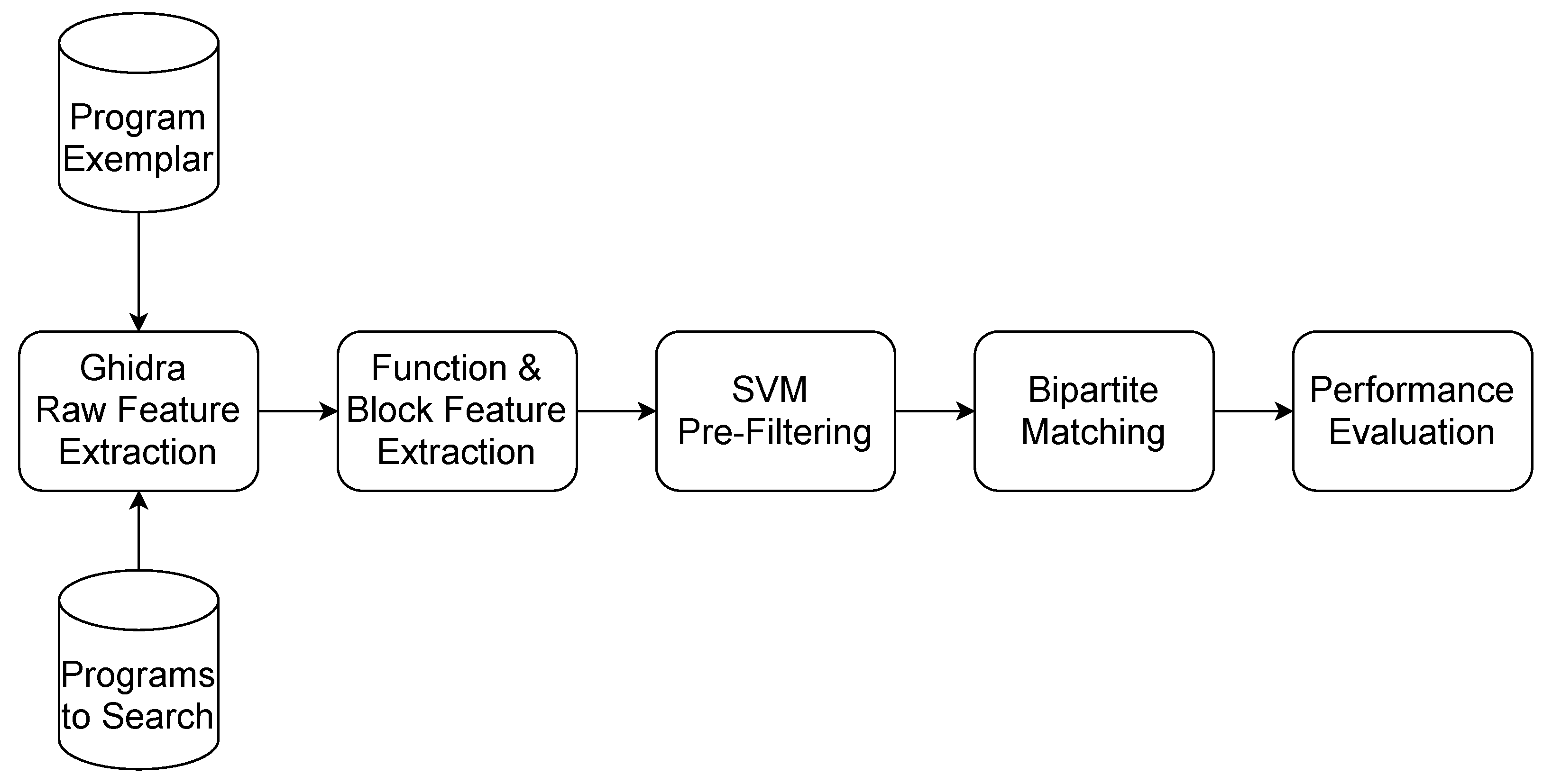
An overview of the CCBVS research is shown in Figure 1. A Ghidra script was written to extract function names and raw features from a program compiled with debugging symbols. The function names are used to generate the ground truth which is used for training, and the assessment of test accuracy. This capability to automatically identify ground truth function pairs allows training to be performed on larger datasets than in the previous studies. The function pairs identified by machine-learning inevitably contain a high false-positive rate. To filter the false positives of each potential function pair, the basic blocks from each function were annotated with features and the Kuhn-Munkres algorithm [13] was used to calculate the minimum matching distance. The Kuhn-Munkres algorithm provides an efficient polynomial-time solution for assignment problems, and more efficient function pair matching than would be possible using graph isomorphism. The calculated similarity of the function pairs was used to filter the matching function pairs. This technique was able to substantially reduce the false positives, and the matching was sufficiently accurate to search for individual functions in different versions of the program created with different compilers.

This research paper makes the following contributions:

• Robust feature engineering for machine-learning based function similarity prediction across different compilers and operating systems.
• Development of a bipartite matching scheme to improve function similarity performance by filtering false-positive function pairs in the SVM model’s output.
• Automatic generation of Function Similarity Ground Truth (FSGT) tables, removing the need for manual reverse engineering.
• Construction of a balanced training dataset built using a duplicated set of all matching function pairs, plus a similar number of randomly selected, non-matching function pairs, resulting in substantially improved program performance.

The structure of this paper is as follows: Section II presents related work, Section III presents the research methodology, Section IV presents the empirical evaluation of results, and Section V presents the conclusion.

2. Related Work

The widespread adoption of IoT devices using open-source code and a variety of CPU architectures provides a requirement for the identification of known vulnerabilities in IoT device firmware. Genius is a vulnerability search database that is used to identify known vulnerable functions in IoT device firmware [14]. First, the IoT firmware is disassembled using the IDA disassembler, and Attributed Control Flow Graphs (ACFGs) were extracted. The following attributes were extracted from the basic blocks in each function.

• Numeric constant count,
• String constant count,
• Transfer instruction count,
• Call count,
• Instruction count,
• Arithmetic instruction count,
• CFG children count,
• CFG Betweenness centrality.

Genius uses bipartite graph matching using the Kuhn-Munkres algorithm [13] to calculate the matching distance between the ACFG of any two functions. An unsupervised spectral clustering algorithm is used to generate a codebook of ACFG clusters, the codebook consists of the set of all centroid nodes. A centroid node is the ACFG possessing a minimum distance to all other ACFGS in the cluster. A function’s raw features are mapped to codebook similarity distances using a feature encoding process. Genius used bag-of-features and Vector of Locally Aggregated Descriptor (VLAD) feature encoding. A Locality Sensitive Hashing (LSH) technique is used to accelerate the searching of encoded features. A MongoDB database was used to store firmware images and encoded images. Datasets were extracted from compiled BusyBox, OpenSSH, and CoreUtils source code, 32-bit programs were compiled for x86, ARM, and MIPS architectures using GCC and Clang compilers with optimization levels 0 to 3.

DiscovRE [7] performs the identification of security vulnerabilities in x86, x64, ARM, and MIPS-based firmware. DiscovRE uses static analysis and provides improved performance over previous dynamic analysis based research. Previous dynamic analysis techniques may not be able to perform analysis of firmware, are limited to single CPU architectures, and make use of semantic similarity techniques that exhibit performance problems with large, compiled images. Security vulnerabilities in open-source code have the potential to impact many IoT devices. This leads to a requirement to identify vulnerable functions in code compiled by different compilers on multiple CPU architectures. DiscovRE identifies vulnerable functions using a two-stage process. The first stage uses the k-Nearest Neighbors algorithm and numerical features to filter functions that may be vulnerable. Feature selection was performed using the Pearson product-moment correlation coefficient [15]. DiscovRE uses the following function counts for stage 1 filtering: function call count, logic instruction count, redirection instruction count, transfer instruction count, local variable count, basic block count, edge count, incoming call count, and instruction count. The second stage identification of vulnerable functions uses Control Flow Graph (CFG) features, and a maximum common subgraph (MCS) algorithm using the McGregor Algorithm [16].

CVSkSA performs a two-stage vulnerable function search in IoT firmware for ARM, MIPS, and x86 CPU architectures, and has higher accuracy, and a faster execution time than previous related research including DiscovRE [8]. The function level features used in the first stage pre-screening were similar to the features used by DiscovRE with the exclusion of redirection instruction count, and transfer instruction count. Two implementations of the first stage were tested, the first implementation uses an SVM model to filter potentially vulnerable functions. A second implementation uses the kNN algorithm for rapid function screening, followed by the SVM model to complete the prefiltering. The use of KNN screening improves the execution time by a factor of four with a slight reduction of accuracy. The second stage uses bipartite graph matching of the function Annotated Control Flow Graphs of the firmware functions. The bipartite graph matching uses the Kuhn-Munkres assignment algorithm with basic block level Attributed Control Flow Graphs (ACFG) [8,14]. The following ACFG features are used: string constant count, function call count, transfer instruction count, arithmetic instruction count, incoming calls count, instruction count, and betweenness.

BugGraph is a two-stage binary code similarity research that can identify functions that are similar to known vulnerable functions [9]. The inputs to BugGraph are a compiled program and the corresponding source code. Stage 1 determines the provenance of the compiled program. The provenance is represented as a canonical representation that consists of {CPU architecture, compiler, compiler version, optimization level} [9]. The Unix file command is used to identify the CPU architecture of the compiled program. A customized version of Origin [17] was used to identify the compiler, compiler version, and optimization level. The supplied source code is then compiled to correspond to the identified toolchain provenance. An Attributed Control Flow Graph (ACFG) was extracted from the functions in each of the programs. BugGraph uses the same attributes as Genius.

The second stage uses a Graph Neural Network (GNN) to provide an embedding for each ACFG. The learning of the GNN was supervised using a graph triplet-loss network (GTN) [18]. A cosine similarity score is used to measure the similarity between the function embeddings produced by the GTN network. The BugGraph GTN is implemented using TensorFlow (TF), and the GNN uses the TF Graph Attention Network. A firmware vulnerability detection experiment was performed using BugGraph. In this experiment, BugGraph was trained using 218 vulnerable functions, six different firmware images were used for vulnerability identification. Vulnerable function candidates were identified by filtering out functions with a similarity score of less than 0.9. These vulnerable function candidates were manually examined to identify 140 OpenSSL vulnerable functions.

The assignment problem deals with how to best assign n workers to m tasks to minimize cost. The assignment problem can be stated as follows [19]:

Minimize:

$$\sum _{i=1}^n\sum _{j=1}^n{c}_{ij}{x}_{ij}$$

(1)

Subject to:

$$\sum _{j=1}^n{x}_{ij}=1,i=1,\dots ,n$$

(2)

$$\sum _{i=1}^n{x}_{ij}=1,j=1,\dots ,n$$

(3)

$$x_{ij}=0or1,i=1,\dots ,nj=1,\dots ,n$$

(4)

where $c_{ij}$ represents the cost of assigning worker i to task j, $x_{ij}$ is 0 or 1, and the total number of tasks is n. Equation (2) indicates that only one worker i can be assigned to each task j, and (3) indicates that each task j should be assigned to only one worker i [19]. The assignment problem can be represented as a bipartite graph with the vertices partitioned into two independent groups, and vertices in the two groups are connected in a 1-1 correspondence that minimizes cost.

The Kuhn-Munkres algorithm is a well-known algorithm for the solution of the assignment problem [20]. This algorithm was developed by Harold Kuhn in 1955 [21], and was reviewed by James Munkres in 1957 [13]. The Kuhn-Munkres algorithm consists of the following steps [20]:

• For each row, subtract the lowest resource cost in that row, from all elements in that row.
• For each column, subtract the lowest resource cost in that column, from all elements in that column.
• Draw the minimum number of lines across rows and columns to cover the zero elements. If the number of tasks matches the number of lines drawn, then the optimal solution has been found.
• If the optimal solution has not been found, find the lowest cell value from the uncovered cells. Subtract this value from each element of all rows with at least one uncovered cell and add this value to each element of the fully covered columns.
• Re-draw the minimum number of lines across rows and columns to cover the zero elements. If the number of tasks matches the number of lines drawn, then the optimal solution has been found.

3. Research Methodology

The CCBVS technique was developed to identify matching functions in a pair of programs compiled with debug symbols for x86/ADM64 architectures. The test programs can potentially be generated with different compilers. The pre-filtering of function pairs was performed using an SVM model, followed by bipartite matching using the Kuhn-Munkes assignment algorithm. The bipartite matching was performed using minimum distance basic block matching to filter false-positive matches.

Ground truth is extracted from the debug symbols of each program and an FSGT table is produced. Labeling of the training dataset and the assessment of the prediction results were performed using the ground truth in the FSGT table. In CCBVS, function similarity features extracted from a pair of programs are used to train an SVM model. The trained SVM model is then used to identify similar functions in subsequent pairs of programs. The accuracy of the function similarity classification is accessed using the ground truth in the FSGT table.

$F_1$ score is used to assess function similarity performance in FSFC [12] and in CCBVS.

Correctly classified similar function pairs are added to the True Positive (TP) count, and correctly classified dissimilar function pairs are added to the True Negative (TN) count. Incorrectly classified dissimilar function pairs are added to the False-Positive (FP) count, and incorrectly classified similar function pairs are added to the False-Negative (FN) count. Precision and recall are calculated from the TP, TN, FP, and FN counts. Precision and recall [22] are defined in Equations (5) and (6), respectively.

$$\mathit{Precision}=\mathit{TP}/\mathit{TP}+\mathit{FP}$$

(5)

$$\mathit{Recall}=\mathit{TP}/\mathit{TP}+\mathit{FN}$$

(6)

The F₁ score (F₁) [22] defined in Equation (7) is used to assess the quality of the results in terms of precision and recall.

$$F_1=2\ast (\mathit{Precision}\ast \mathit{Recall})/(\mathit{Precision}+\mathit{Recall})$$

(7)

3.1. Training Algorithm

The training algorithm identifies matching function pairs using the FSGT table, and then extracts features for each pair of matching functions and extracts features from an equal number of randomly selected non-matching function pairs. The training algorithm used in CCBVS is faster than the method used in the previous Function Similarity Using Family Context (FSFC) [12] research and generates a balanced training dataset.

3.2. SVM Model Features

The following function similarity features were extracted from each function for use by the SVM model:

• Set of API calls,
• Function calls count,
• Push count,
• Set of constants,
• Stack size,
• Basic block count,
• Arithmetic instructions count,
• Lea instruction count.

CCBVS uses features from FSFC [12], apart from the return release count, which is only present in code the uses a CDECL calling convention. The push instruction count, arithmetic instruction count, and lea instruction count features were added to CCBVS.

API calls: The API call feature $AC$ is defined in FSFC [12], but in CCBVS this feature refers to either Linux library function calls or to Windows API calls.

Function calls count: The function calls count feature $FC$ is defined in FSFC [12].

Constants: The constants feature $CS$ is defined in FSFC [12].

Stack size: The stack size feature $SS$ is defined in FSFC [12].

Basic block count: The basic block count feature $BB$ is defined in FSFC [12].

Push instruction count: Let PC be the count of push instructions psh within a function f in a program p.

$$PC(f,p)=|\{ps{h}_0,ps{h}_1,\dots ,ps{h}_{\mathrm{m}}\}|$$

(8)

Arithmetic instruction count: Let RC be the count of arithmetic instructions ar within function f in program p. Arithmetic instructions are taken to be the set of all ADD, SUB, INC, DEC, MUL, DIV, ADC, SBB, and NEG instructions.

$$RC(f,p)=|\{a{r}_0,a{r}_1,\dots ,a{r}_{\mathrm{q}}\}|$$

(9)

LEA instruction count: Let LC be the count of LEA instructions l within function f in program p.

$$LC(f,p)=|\{l_0,l_1,\dots ,l_{\mathrm{r}}\}|$$

(10)

3.3. Function Context

Previous research [11,12] has shown that the use of function context results in a substantial strengthening of the function similarity features used in the SVM model. Features from a function’s context consist of the features from the function under consideration, plus features from a set of closely associated functions. In CCBVS, three levels of function context are defined: Self (S), Child (C), and Parent (P).

The Self (S) context of function f is the set of the non-API functions that are called from function f.

$$S\left(f\right)=\{s_0,s_1,\dots ,s_{\mathrm{i}}\}$$

(11)

The set of functions in the Child context C of function f can be obtained by iterating through each of the functions in the Self context of f and extracting the non-API functions.

$$C\left(f\right)=\{s\left(f^{\prime }\right)\forall f^{\prime }inS\left(f\right)\}$$

(12)

The functions in the Parent context P of function f is the set of non-API functions that call function f.

$$P\left(f\right)=\{p_0,p_1,\dots ,p_{\mathrm{j}}\}$$

(13)

3.4. Feature Ratios

Feature ratios are calculated for each potential function pair in the test and training datasets. A feature ratio is the Jaccard index for the corresponding features of a function pair. For example, the API feature ratio is the Jaccard index of the set of API functions in each function of the pair being compared.

The following feature ratios are defined in FSFC [12].

• API Ratio—$ACR$,
• Function Calls Ratio—$FCR$,
• Constants Ratio—$CSR$,
• Stack Ratio—$SSR$,
• Blocks Ratio—$BBR$.

Push Count Ratio: Let $P{C}_1$ and $P{C}_2$ be the sets of all push instruction counts extracted from the context of each of the functions in the function pair fp. Let the Push Count Ratio $PCR$ be the Jaccard index of $P{C}_1$ and $P{C}_2$.

Arithmetic Instruction Count Ratio: Let $R{C}_1$ and $R{C}_2$ be the sets of all arithmetic instruction counts extracted from the context of each of the functions in the function pair fp. Let the Arithmetic Instruction Count Ratio $RCR$ be the Jaccard index of $R{C}_1$ and $R{C}_2$.

Lea Instruction Count Ratio: Let $L{C}_1$ and $L{C}_2$ be the sets of all Lea instruction counts extracted from the context of each of the functions in the function pair fp. Let the Lea Instruction Count Ratio $LCR$ be the Jaccard index of $L{C}_1$ and $L{C}_2$.

3.5. Bipartite Matching

The goal of the filtering step is to remove function similarity predictions that are false positives. An obvious method to perform filtering would be to check the CFG isomorphism of the predicted function pair. However, graph isomorphism is computationally expensive and is not able to be solved in polynomial-time (NP) [23]. Another approach to testing function similarity is to treat this problem as an assignment problem where the goal is to determine an optimum assignment of basic blocks that minimizes difference. The selection of those functions with the minimum basic block difference can be used to filter false-positive predicted function matches from the SVM model. While the features used in the SVM model are defined as function attributes, the features used in bipartite matching are defined as basic block attributes.

Function Basic Block Set: Let FBBS be the set of all basic blocks b within function f in program p.

$$FBBS(f,p)=\{b_0,b_1,\dots ,b_{\mathrm{q}}\}$$

(14)

Each basic block b is labeled with the following features:

• Set of API names,
• Function call count,
• Push instructions count,
• Set of constants,
• Arithmetic instructions count,
• Lea instruction count.

Basic Block API Calls: Let ACBB(f, p, b) be the set of API functions called from basic block b in function f in program p.

$$ACBB(b,f,p)=\{a_0,a_1,\dots ,a_{\mathrm{r}}\}$$

(15)

Basic Block Function Calls Count: Let FCBB be the count of function call instructions c within basic block b in function f in program p.

$$FCBB(b,f,p)=|\{c_0,c_1,\dots ,c_{\mathrm{s}}\}|$$

(16)

Basic Block Push Instruction Count: Let PCBB be the count of push instructions psh within basic block b in function f in program p.

$$PCBB(p,f,p)=|\{ps{h}_0,ps{h}_1,\dots ,ps{h}_{\mathrm{t}}\}|$$

(17)

Basic Block Constants: Let CSBB(b, f, p) be the set of constants k that are not program or stack addresses within basic block b in function f in program p.

$$CSBB(b,f,p)=\{k_0,k_1,\dots ,k_{\mathrm{u}}\}$$

(18)

Basic Block Arithmetic instruction count: Let ACBB be the count of arithmetic instructions ar within function f in program p. Arithmetic instructions is taken to be the set of all ADD, SUB, INC, DEC, MUL, DIV, ADC, SBB, and NEG instructions.

$$ACBB(b,f,p)=|\{a{r}_0,a{r}_1,\dots ,a{r}_{\mathrm{v}}\}|$$

(19)

Basic Block LEA instruction count: Let LCBB be the count of LEA instructions l within basic block b in function f in program p.

$$LCBB(b,f,p)=|\{l_0,l_1,\dots ,l_{\mathrm{w}}\}|$$

(20)

Function Basic Block Attributes: Let FBBA be the map of each function to the following basic block features:

• Basic Block API Calls
• Basic Block Function Calls Count
• Basic Block Push Instruction Count
• Basic Block Constants
• Basic Block Arithmetic Instruction Count
• Basic Block LEA Instruction Count

$$\begin{array}{c}\hfill FBBA(b,f,p)=\{ACBB,FCBB,PCBB,\\ \hfill CSBB,ACBB,LCBB\}\end{array}$$

(21)

The matching distance d between basic block b₁ and b₂ is calculated using the method given in CVSkSA [8], where ${\alpha }_{1i}$ and ${\alpha }_{2i}$ are the ith features of the predicted function pair, and ${\omega }_i$ is the weight of the ith feature.

$$d(b_1,b_2)=\frac{{\mathsf{\Sigma }}_i{\omega }_i|{\alpha }_{1i}-{\alpha }_{2i}|}{{\mathsf{\Sigma }}_i{\omega }_{i}max({\alpha }_{1i},{\alpha }_{2i})}$$

(22)

The Kuhn-Munkres algorithm is used to calculate the approximate minimum matching distance between predicted function pairs by calculating a bipartite graph matching G = (V,E) where V is the set of functions f from each program (p1, p2). E is the set of edges associated with the predicted function pairs, each edge is assigned the approximate minimum matching distance mmd calculated by the Kuhn-Munkres algorithm (KM).

$$MMD=KM\left(D\right)$$

(23)

The approximate similarity $\mathsf{\Psi }$ between a function pair is calculated using the method given in CVSkSA [8].

$$\mathsf{\Psi }(f_1,f_2)=1-\frac{mmd(f_1,f_2)}{min(mmd(f_1,\varnothing ),mmd(f_2,\varnothing )}-p\times n$$

(24)

where $\mathsf{\Psi }(f_1,f_2)$ is the similarity between the Functions f₁, and f₂, d(f₁,f₂) is the approximate minimum matching distance between functions f₁ and f₂, and ∅ is a size conformant null FBBA. This calculation of similarity includes a penalty term to exclude function pairs with a large difference in basic block count, p is a penalty factor and n is the difference in basic block count in the predicted function pair. The matching functions are selected using the approximate function similarity value.

4. SVM Model Evaluation

4.1. Removal of External Dependencies

The CCBVS technique uses Ghidra to disassemble compiled programs. A script was written to save this information in a python format that includes the disassembled instructions, function names, and API names. Previous research used Cythereal facilities for malware unpacking and disassembly. However, problems with Cythereal availability prompted the switch to Ghidra based analysis. The format of the disassembled code extracted from Ghidra differs from the IDA disassembly from Cythereal. The function similarity program was updated to process the Ghidra format.

4.2. Ground Truth Generation

CCBVS uses an FSGT table, this ground truth table may be created either automatically or by manual reverse engineering. The automated creation of the FSGT table uses open-source programs that are compiled with debugging symbols. The debugging symbols allow the Ghidra feature extraction script to include function names in the disassembled code. This automatic generation of ground truth function matches allows the use of larger datasets than the research using a manually created FSGT table.

4.3. Datasets

The following datasets were used in this research:

• Zeus malware,
• ISFB malware,
• BusyBox,
• Linux OpenSSL version 1.1.1,
• Windows OpenSSL version 1.1.1.

The Zeus and ISFB datasets were created in previous research. The ground truth for these datasets was established using malware reverse engineering and leaked source code [11]. The compiler for these malware datasets is consistent with Visual Studio. The BusyBox dataset was created by cross-compiling with GCC on Linux to create a PE32 program. OpenSSL version 1.1.1 was compiled with GCC on Linux to create a 64-bit ELF program. OpenSSL version 1.1.1 was compiled with Visual Studio on Windows to create a PE32 program. The OpenSSL datasets were extracted from the libcrypto binary.

4.4. Statistical Significance

The statistical significance tests used in FSFC [12] were used to assess the statistical significance of the CCBVS results. A Shapiro-Wilk [24] test was performed to determine whether the results from experiment 1 were normally distributed. A p-value of 0.00002 indicated that the results were not normally distributed, and a two-tailed Wilcoxon signed-rank test [25] was used to determine whether the test results differed at a 95% level of confidence.

4.5. Imbalanced Test Dataset

CCBVS used the same function similarity prediction algorithm as FSFC [12]. In this research, function similarity was tested using the Cartesian product of the functions in each of the two test datasets. This technique generates an imbalanced test dataset. FSFC showed that using a random classifier with the Zeus dataset, an $F_1$ score of similar function prediction would be 0.0034 [12]. The CCBVS $F_1$ scores are well above those that would be expected using random classification.

4.6. Training Dataset

Experiments are performed in this section to test the performance of our SVM model. These experiments use the same set of function level features, these are API Ratio $ACR$, Function Calls Ratio $FCR$, Constants Ratio $CSR$, Stack Ratio $SSR$, Blocks Ratio $BBR$, Push Count Ratio $PCR$, Arithmetic Instruction Count Ratio $ACR$, and the Lea Instruction Count Ratio $LCR$.

In this research, the training dataset was developed by selecting features corresponding to the matching function pairs, and an equal number of randomly selected, non-matching function pairs. An experiment was performed to test the effect of the duplication of non-matching function pairs in the training dataset. The results of this experiment are provided in

Table 1. Non-Matching Function Pair Duplication Test.

Duplication Count	Average ${\mathit{F}}_1$ Score	S.D.	p-Value
1	0.3805	-
10	0.4325	Y	0.00988
30	0.4405	N	0.44726

. These results show that function similarity performance increases as the training features are duplicated, and the best performance is reached with 10 duplicates of each non-matching function pair. In Table 1, a value of “Y” in the column labeled “S.D.” indicates that the current result is significantly different from the preceding result. The column labeled “p-value” provides the p-values of the two-tailed Wilcoxon signed-rank test of this comparison. The SciKit-Learn Linear SVC SVM model was used in this research.

4.7. Verification

Function similarity prediction was performed using the Zeus and ISFB malware datasets from FSFC was used to verify the performance of the modified script [12]. The results of this verification test are shown in

Table 2. Zeus/ISFB SVM Model Verification.

Test Runs	Average ${\mathit{F}}_1$ Score
20	0.43

with the use of all features. These results show an average $F_1$ score of 0.43, this value is not significantly different from the previous FSFC research [12] and demonstrates that the new training method has not impacted the SVM model performance.

4.8. Feature Strength

The strength of individual features was assessed by testing on the Zeus and ISFB datasets from FSFC. The results of this experiment are shown in

Table 3. Zeus/ISFB Individual Feature Performance.

Test Runs	Feature	Average ${\mathit{F}}_1$ Score
20	API Ratio $ACR$	0.06
20	Lea Instruction Count Ratio $LCR$	0.05
20	Arithmetic Instruction Count Ratio $RCR$	0.07
20	Block Ratio $BBR$	0.22
20	Stack Ratio $SSR$	0.01
20	Constants Ratio $CSR$	0.17
20	Push Count Ratio $PCR$	0.18
20	Function Calls Ratio $FCR$	0.16

. The highest performing feature combinations are shown in

Table 4. Zeus/ISFB Highest Performing Feature Combinations.

Test Runs	Vector	Average ${\mathit{F}}_1$ Score
5	01010110	0.59
5	01010111	0.59
5	01011111	0.59
5	01110100	0.58
5	01110101	0.59
5	01110110	0.61
5	01110111	0.59
5	01111110	0.58
5	01111111	0.58
5	11010110	0.58
5	11110110	0.58

, where the best performing features were: Arithmetic Instruction Count Ratio $RCR$, Stack Ratio $SSR$, Push Count Ratio $PCR$, and the Function Calls Ratio $FCR$.

The features used in these experiments were assigned a binary identifier, this binary encoding method allows the numbering of individual tests. This feature numbering scheme is shown in

Table 5. Identification of Feature Combination Tests.

Feat #	Vector	Description
1	00000001	API Ratio $ACR$
2	00000010	Function Calls Ratio $FCR$
4	00000100	Push Count Ratio $PCR$
8	00001000	Constants Ratio $CSR$
16	00010000	Stack Ratio $SSR$
32	00100000	Block Ratio $BBR$
64	01000000	Arithmetic Instruction Count Ratio $RCR$
128	10000000	Lea Instruction Count Ratio $LCR$

.

4.9. Training with BusyBox Features

Features extracted from the BusyBox dataset were used to train an SVM model that was used to predict similarity in the ISFB malware dataset. The results of this test are shown in

Table 6. ISFB Similarity Using BusyBox Features.

Test Runs	Average ${\mathit{F}}_1$ Score
20	0.30

. These results show that an SVM model using features from PE32 code compiled with GCC can be used to predict function similarity in a program compiled with Visual Studio.

4.10. Training with Visual Studio OpenSSL Features

Features were extracted from libcrypto.dll in OpenSSL version 1.1.1, which was compiled as a PE32 program using Visual Studio. These features were used to train an SVM model that was used to predict similarity in the ISFB malware dataset. The results of this test are shown in

Table 7. ISFB Similarity Using OpenSSL Features.

Test Runs	Average ${\mathit{F}}_1$ Score
20	0.17

. These results show that an SVM model using features from PE32 code compiled for Visual Studio can predict function similarity in a PE32 program compiled with Visual Studio.

4.11. Training with Linux OpenSSL Features

Features were extracted from libcrypto.dll in OpenSSL version 1.1.1, which was compiled as a 64-bit ELF program on a Linux workstation. These features were used to train an SVM model that was used to predict similarity in the ISFB malware dataset. The results of this test are shown in

Table 8. ISFB Similarity Using Linux OpenSSL Features.

Test Runs	Average ${\mathit{F}}_1$ Score
20	0.72

. These results show that the SVM model using features from elf 64-bit code can predict function similarity in a PE32 program compiled with Visual Studio.

4.12. OpenSSL Training—Busybox Test

Features from the OpenSSL version 1.1.1 Linux data set were used to train the SVM model to predict similarity in the BusyBox dataset. The results of this test are shown in

Table 9. BusyBox Similarity Using OpenSSL Features.

Test Runs	Average ${\mathit{F}}_1$ Score
20	0.45

. These results help to build the case that machine-learning can predict function similarity in compiled C code, benign programs, and malware.

4.13. SVM Model Summary

The automatic generation of the ground truth used in CCBVS allows evaluation with a wider range of programs, allowing experiments to be conducted to examine whether features from a range of x86, and Intel 64 compilers can be used to predict function similarity. The above experiments show that the SVM model can abstract features from programs compiled with a range of compilers and formats and can predict function similarity in both malware and benign programs.

5. Bipartite Matching Evaluation

The function similarity results generated by the SVM model contain a substantial number of false positives. A bipartite matching method uses the Kuhn-Munkres algorithm to filter false positives from the predicted function matches. This bipartite matching method is based on the method from CVSkSA [8]. In this technique, the Kuhn-Munkres algorithm is used to find the lowest cost matching distance between the basic blocks of a function pair. The similarity of the CFGs of the function pair is calculated, and this is used to filter false-positive function pairs.

Equation (24) contains a term that penalizes similarity where the basic block count of a predicted function pair differs substantially. This experiment identifies the penalty value that provides the best function similarity performance, the results of this experiment are shown in

Table 10. Effect of Penalty Factor on Accuracy.

Test Runs	Penalty Factor	Average ${\mathit{F}}_1$ Score	S.D.	p-Value
20	0.00	0.83	-	-
20	0.10	0.88	Y	0.00008
20	0.20	0.87	Y	0.0002
20	0.30	0.87	N	-
20	0.40	0.87	N	-

.

The two-tailed Wilcoxon signed-rank test calculator was not able to provide an accurate p-value for the tests of significant difference between penalty factors 0.20 and 0.30, and 0.30 and 0.40. Thus, it is concluded that these results do not differ at a 95% level of significance.

The best function similarity accuracy is achieved with a penalty factor of 0.10, which is significantly different from adjacent values.

Experiments were performed in this section to test the combined performance of our SVM model and the second stage bipartite filtering. These experiments use the basic block features provided by the Function Basic Block Attributes $FBBA$.

5.1. Exclusion of Small Functions

During testing of the SVM model, it was noted that a high proportion of false positives occur when the basic block count of the functions being compared was less than three basic blocks. CVSkSA [8] and DiscovRE [7] exclude functions containing less than five basic blocks. For consistency, the bipartite matching method in this paper excludes functions with less than five basic blocks.

An experiment was performed where functions with less than five basic blocks were excluded. The training was performed using features from the Linux OpenSSL dataset, and testing was performed using features from the BusyBox dataset. The results of this experiment are shown in

Table 11. BusyBox Similarity, Excluding Small Functions.

Test Runs	TP	FP	TN	FN	${\mathit{F}}_1$ Score
1	729	912	752520	100	0.59

. The average $F_1$ score for this dataset in the presence of small functions was 0.45 in Table 9, when small functions were excluded, the $F_1$ score rose to 0.59.

5.2. Function Similarity Value

The Kuhn–Munkres algorithm is used to calculate the minimum matching distance between the two functions, then the similarity of the two functions is calculated using the CVSkSA method [8]. If the function similarity score is greater than a matching threshold value, then a function match is declared. To determine the best matching value, a test was performed using the Linux OpenSSL SVM model to predict similarity in BusyBox using different matching threshold values. The results of this experiment are shown in

Table 12. Effect of Matching Threshold.

Test Runs	Matching Threshold	${\mathit{F}}_1$ Score
1	0.1	0.75
1	0.2	0.77
1	0.3	0.80
1	0.4	0.84
1	0.5	0.86
1	0.6	0.89
1	0.7	0.90
1	0.8	0.91
1	0.9	0.91

. The remaining experiments use a matching value of 0.8.

5.3. Bipartite Matching Weights

In the bipartite matching method, each feature is assigned a weight. The purpose of the weights is to minimize the distance between similar functions and to maximize the distance between different functions [8]. Weight values between 0.05 and 100 were tested. The selected weights were those that provided the highest $F_1$ Score and the lowest false-positive count. The selected weights are shown in

Table 13. Bipartite Matching Weight Selection.

Feature	Description	Weight	${\mathit{F}}_1$ Score
$ACBB$	API Calls	10	0.85
$FCBB$	Call Count	45	0.81
$FCBB$	Push Count	20	0.84
$CSBB$	Constants Count	5	0.82
$ACBB$	Arith Ins Count	50	0.85
$LCBB$	Lea Ins Count	95	0.81

. This experiment used the ISFB dataset for training and the Busybox dataset for testing.

5.4. Bipartite Matching Results

The bipartite matching method was applied to the datasets used in the SVM model evaluation. The results are shown in

Table 14. Bipartite Matching Results.

Test Runs	Train Dataset	Test Dataset	${\mathit{F}}_1$ Score
20	Zeus	ISFB	0.89
20	BusyBox	ISFB	0.90
20	VS OpenSSL 1-1-1	ISFB	0.89
20	Linux OpenSSL 1-1-1	ISFB	0.82
20	Linux OpenSSL 1-1-1	BusyBox	0.91

and show a substantial reduction in false positives over the SVM model only results. Earlier research in CVCFS [11] employed an edit distance of Cythereal semantics to filter function similarity results. The CVCFS edit distance technique used a Zeus dataset and gave a maximum $F_1$ Score of 0.78. The $F_1$ score values are shown in Table 14 and give an average $F_1$ score of 0.88, which is a significant improvement.

5.5. Single Function Search

The use of bipartite matching substantially improves the function matching performance. This experiment tests the ability of the research to match individual functions. The results of this experiment are shown in

Table 15. Single Function Search Results.

Function	Train Dataset	TP	FP	${\mathit{F}}_1$
c2i_ASN1_OBJECT	ISFB	1	0	1.00
EVP_DecodeUpdate	ISFB	1	0	1.00
X509_cmp_time	ISFB	1	0	1.00
c2i_ASN1_OBJECT	BusyBox	1	0	1.00
EVP_DecodeUpdate	BusyBox	1	0	1.00
X509_cmp_time	BusyBox	1	0	1.00
c2i_ASN1_OBJECT	Mingw OpenSSL 1.1.1	1	0	1.00
EVP_DecodeUpdate	Mingw OpenSSL 1.1.1	1	0	1.00
X509_cmp_time	Mingw OpenSSL 1.1.1	1	0	1.00
c2i_ASN1_OBJECT	Linux OpenSSL 1.1.1	1	0	1.00
X509_cmp_time	Linux OpenSSL 1.1.1	1	0	1.00
EVP_DecodeUpdate	Linux OpenSSL 1.1.1	1	0	1.00

, These results show that CCBVS can search for specific single functions. The function selected were taken from OpenSSL version 1.1.1A and OpenSSL version 1.1.1H. These programs were compiled as PE32 with Visual Studio. These functions are three of the vulnerable functions that were used in the CVSkSA tests [8]. It is acknowledged that these functions are not vulnerable in OpenSSL version 1.1.1, however, they are representative of the functions used in the CVSkSA research [8].

5.6. CCBVS Evaluation

This research provides a substantial improvement over the previous research in the following areas:

• Removal of external dependencies,
• Improved training dataset generation,
• Automated ground truth generation,
• Improved execution time,
• Improved function similarity performance.

Previous FSFC function similarity research made use of the disassembly in the BinJuice semantics provided by Cythereal. In the CCBVS research, a decision was taken to use Ghidra scripting to extract a disassembly in a similar format to the BinJuice semantics. The outcome of this change is the removal of an external dependency.

The FSFC function similarity research builds the training dataset using a pairwise (n${}^2$) combination of all functions in the two programs being compared. The CCBVS research builds the training dataset based on the features from all of the matching function pairs and an equal number of randomly selected, non-matching function pairs. This new method of creating the training dataset has similar accuracy to that of the FSFC research, but the substantially smaller training dataset results in improved run-time. The experiments in this research were performed using a workstation with an Intel i7-3770 processor with a base frequency of 3.40 GHz, a peak frequency of 3.90 GHz, four cores, eight threads, and 32 GB of RAM.

Previous research required the manual creation of the FSGT table. CCBVS extracts features with function names taken from debug symbols. The feature extraction script uses the Ghidra facility to load the .pdb debug symbol file. This allows the extraction of function names from debug symbols. The automated generation of ground truth allows experiments to be conducted with a wider range of programs than was possible with previous research, allowing larger training datasets and improved accuracy.

Previous research used an SVM model implemented using Tensor Flow. This SVM model ran for a specific number of training iterations. The CCBVS research uses the SciKit-Learn Linear SVC SVM model. This model runs until a specified stopping criteria tolerance is reached. This use of the stopping criteria contributes to a substantial reduction in run-time.

Table 16. Zeus/ISFB Dataset Run-Time Comparison.

Operation	Dataset	Feature Extraction (s)	SVM (s)
FSFC Train	Zeus	13	1330
FSFC Classify	ISFB	37	357
CCBVS Train	Zeus	3.3	0.1
CCBVS Classify	ISFB	37.0	4.9

, provides a comparison of the run-time performance of CCBVS with that of FSFC. This experiment uses training with features from the Zeus dataset and function similarity prediction with features from the ISFB dataset. This specific dataset was used to allow direct comparison with the FSFC run-time. These results show the SVM model had a total run-time of 45.3 s, an improvement by a factor of 38.

The total run-time including bipartite matching of this dataset was 55 s. It is noted that although the number of training records has been reduced from n${}^2$ to linear, SVM model prediction is still performed for all combinations of the functions in the two samples being compared.

6. Future Work

The research presented in this paper can be extended as follows:

• Extend this research to identify similar functions in compiled C++ code.
• Update similarity techniques for general cross-architecture function similarity.
• Improve the testing technique to decrease the false-positive rate in large programs by avoiding pairwise (n${}^2$) function comparison.
• Evaluate several machine-learning techniques to identify the best performing method.

7. Conclusions

The matching of similar compiled functions is important in the following activities, the triage of malware, analysis of program patches, identification of library functions, analysis of code authorship, the identification of similar function pairs to reduce manual analysis workload, plagiarism analysis, and vulnerable function identification.

The addition of an automated method for the generation of ground truth allows this research to identify similar functions in open-source programs compiled with debugging symbols. This removal of the need for manual reverse engineering to generate ground truth allows experimentation with machine-learning function similarity techniques on a wide range of datasets.

This paper has presented techniques to improve the runtime of the training algorithm by a factor of 38. The addition of a bipartite matching method reduces false-positive matches and provides an average $F_1$ score of 0.88.

This research further demonstrates the feasibility of machine-learning function similarity techniques and builds the case that machine-learning could be used as the basis for a general purpose function similarity engine.