Analyzing and Visualizing Deep Neural Networks for Speech Recognition with Saliency-Adjusted Neuron Activation Profiles

Abstract

Deep Learning-based Automatic Speech Recognition (ASR) models are very successful, but hard to interpret. To gain a better understanding of how Artificial Neural Networks (ANNs) accomplish their tasks, several introspection methods have been proposed. However, established introspection techniques are mostly designed for computer vision tasks and rely on the data being visually interpretable, which limits their usefulness for understanding speech recognition models. To overcome this limitation, we developed a novel neuroscience-inspired technique for visualizing and understanding ANNs, called Saliency-Adjusted Neuron Activation Profiles (SNAPs). SNAPs are a flexible framework to analyze and visualize Deep Neural Networks that does not depend on visually interpretable data. In this work, we demonstrate how to utilize SNAPs for understanding fully-convolutional ASR models. This includes visualizing acoustic concepts learned by the model and the comparative analysis of their representations in the model layers.

1. Introduction

Artificial Neural Network (ANNs) have become a very popular tool for solving challenging tasks across various fields of application. Increasing their performance is often achieved through increasing their depth, the number of neurons or by using more complex architectures [1]. At the same time, larger computational models become black-boxes, which are harder to interpret [2]. This complicates detecting erroneous behavior, thus can be risky in critical applications. Several introspection techniques have been proposed to obtain insight into ANNs [3,4]. However, most introspection methods are designed for certain applications or architectures. In particular, many introspection techniques focus on images because the features of images are easy to interpret visually. Features in the audio domain are more difficult to interpret visually, making established introspection techniques less suitable for understanding the model. In this work, we address the consequent need for methods to also understand ANNs that process data which are not visually interpretable.

The complexity of ANNs is becoming closer to that of real brains. While complex ANNs are a recent technical development, real brains have been studied in neuroscience for over 50 years. This rich experience from the field of neuroscience can also help to understand complex ANNs better. By adapting well-established methods that are used for understanding real brain activity it is possible to analyze ANNs, as well [5]. In this work, we particularly take inspiration from a popular technique in the field of neuroscience, the Event-Related Potential (ERP). The ERP technique is used for analyzing brain activity through Electroencephalography (EEG) [6]. ERPs aim to measure brain activity for a particular fixed event (stimulus). As the event is consistent across all EEG measurements, aligning the data at this stimulus and averaging the signals yields event-specific  information [7]. Averaging of a random signal over multiple measurements, in contrast, is returning the expected value of its random distribution. This way, in ERPs, variations in brain activity that are unrelated to the stimulus are removed from the measurements. We analyze ANNs similarly, but as their responses are deterministic, we use the averaging to remove particular variations in the input data. For example, in a speech recognition model, we characterize ANN responses to a particular phoneme by using averaging to remove the variation that originates from different speakers and articulations.

In this work, we present Saliency-Adjusted Neuron Activation Profile (SNAPs) as an ERP-inspired analysis of ANNs. SNAPs build on our earlier research in which we already introduced specific aspects of the methodology [8,9]. Here, we extend and generalize these techniques to be useful for a wider range of analyses of ANNs. Furthermore, we perform a validation of the individual steps in the SNAP computation procedure. SNAPs themselves are characteristic responses of ANNs to particular groups of inputs. They can be used for various ways of performing a comprehensive analysis of the network. We showcase two exemplary ways to utilize SNAPs for examining network responses using fully-convolutional Automatic Speech Recognition (ASR) models: 1. Interpreting visualized SNAPs directly and 2. Analyzing representations in any layer of the network using a clustering-based approach.

With SNAPs, we introduce a novel technique to analyze and visualize ANNs which, in contrast to most established introspection techniques, does not require visually interpretable input data. In particular, our method focuses on describing the behavior of the model. How to use the results for improving the model will be discussed, but specific experiments are outside the scope of this work.

2. Related Work

2.1. ASR Using Convolutional Neural Networks

Machine Learning (ML) comprises algorithms that are designed to use data to automatically improve themselves. Therefore, ML algorithms can learn to perform tasks which are too complex to be implemented with manual instructions. One common ML task is supervised learning, where the model learns to predict labels from a given labeled data set. Supervised learning tasks are, for example, classification, regression or transcription. In unsupervised learning tasks, the ML model analyzes unlabeled data with the aim of capturing the structure of the data [10]. For example, in clustering tasks, data are grouped according to their similarities.

Deep Learning (DL) is a branch of machine learning that uses ANNs with multiple layers. An ANN consists of many artificial neurons, each computing a weighted sum of its connected inputs and applying a non-linear function to the result. These neurons are organized in a series of hidden layers, where typically only neurons of successive layers are connected but not neurons of the same layer. Each connection is weighted by a trainable parameter. Because of the huge number of connections, resulting from having several hidden layers, ANNs need massive amounts of data as input to learn suitable connection weights for performing correct predictions for the inputs. DL allows us to automatically learn feature representations by learning simple patterns in the early layers and combining them to increasingly complex patterns in the deeper layers. The learning procedure of an ANN is to minimize its prediction error by updating the connection weights between neurons with optimization algorithms like Gradient Descent or Adam [11,12].

Convolutional Neural Network (CNNs) are a type of DL architecture which can detect patterns independent of their position in the input. This is achieved by convolving the input with trainable filters. The receptive field of a filter describes the region in the input used to compute a single output value of the convolution layer. The receptive field of filters in deeper layers can be propagated back to the input. Correspondingly, the receptive field of the output layer is the part of the input that is used for one prediction. Convolutions are typically applied to consecutive regions in the input. For reducing the resolution of the output, convolution can be applied with a stride of s, meaning that it is applied to every sth region. The output of applying one convolution filter to the complete input is called a feature map [11].

Usually, for two-dimensional data like images, CNNs with two-dimensional filters are used. For operating on one-dimensional data, CNNs with one-dimensional filters are preferred over 2D CNNs because of the lower computational complexity [13]. As speech is a one-dimensional signal, one of the applications of 1D CNN is in speech recognition. A 1D CNN can operate directly on a signal or on a spectrogram, which is a representation of frequencies of a signal during the time [13,14,15]. Each time step of a spectrogram corresponds to an overlapping time interval in which the peak amplitude of a set of frequency bins is derived. The resulting values are commonly referred to as the intensities of the frequencies [16].

Using CNNs for speech recognition is not uncommon [17,18] but is often combined with models from traditional ML or other DL models. For example, such hybrid models involve Hidden Markov Models [19,20] or Recurrrent Neural Network (RNNs) [21]. Besides ASR, CNNs are also used for other speech-related tasks, for example learning spectrum feature representations [22] or speech emotion recognition [23].

2.2. Model Introspection

Model introspection is the process of analyzing or visualizing internal structures or processes of computational models. This is of particular interest in DL models as these work as black-boxes [2]. Research on elucidating DL model internals has gained traction recently and several introspection techniques have been proposed. However, most research is done in the field of computer vision due to the ease of visual inspection [3,4,24].

2.2.1. Feature Visualization

A simple way of inspecting internal structures of a DL model is to visualize its learned weights. In fully-connected neural networks, each neuron in the first hidden layer is connected to all values in the input. To inspect the pattern that a particular neuron in this layer responds to, the weights of these connections can be visualized. To this end, the weight values are plotted according to the position of the corresponding values in the  input [25]. For image data or spectrogram inputs, the weights are visualized as image, too. In time-series data like speech recordings, weight visualization follows the one-dimensional structure of the input. In deeper layers, neurons receive input signals from neurons in the preceding hidden layer. Neurons within the same layer are not interconnected and therefore have no informative ordering. Hence, in deeper layers, plotting the connection weights cannot be interpreted by visual inspection.

In CNNs, weights are applied as convolution operations with usually very small filters. For example, $3\times 3$ is a common size of filters in 2D CNNs. For such small filters, it is almost impossible to understand their learned features only by visual inspection of the plotted weights. Thus, instead of visualizing weights, feature maps of CNNs can be visualized. A feature map comprises all neuron activations corresponding to the same convolutional filter. Each position in the feature map only shows how strongly this convolutional filter activates for the corresponding region of the input. Therefore, feature maps only reveal to which part of the input a filter is responding but do not visualize the pattern which this filter detects [2].

A common way for visualizing the features learned in deeper layers is to create an input which maximally activates individual neurons or sets of neurons [2,26,27]. Such input is obtained by an optimization procedure similar to the ANN training. In ANN training, parameters of the network are updated to decrease the prediction error. For feature visualization, input values are updated to increase the activation values of a target set of neurons. In CNNs, complete feature maps are typically used as the target set of neurons. For brevity, we refer to the obtained inputs as “optimized inputs”. Optimized inputs can differ substantially from instances in the training data, making them difficult to interpret. For human perception, optimized inputs of images often look unrealistic. Optimized inputs in the speech domain often do not sound like natural speech or do not look like spectrograms of natural speech [8,28]. This problem can be tackled by applying regularization techniques to the optimization. Regularization adds constraints which, in addition to increasing activation of neurons of interest, encourage the optimized input to be more similar to natural data. For example, a spectrogram of natural speech does not contain a wide range of frequencies of high intensity over longer time spans. To discourage such patterns in optimized inputs, a high number of large values needs to be avoided. This can be achieved by penalizing the sum of absolute values in the input during the optimization. In the field of ML, this technique is known as $L_1$ regularization. Stronger regularization techniques encourage optimized inputs to be more similar to data examples. Although this leads to more natural visualizations, they might not represent the learned features well. For example, additionally minimizing the distance to a data example encourages the optimized input to be more natural but makes it impossible to detect whether a filter also reacts to unrealistic patterns.

2.2.2. Saliency Maps

The strategy of another type of typical introspection techniques is to explain how a prediction for a single input example was made. To this end, such methods quantify how relevant each individual value in this input example is for the prediction [3,4,26,29,30,31,32]. To visualize the obtained relevance values, they are commonly plotted as heat map overlaid on top of the input. This heat map of relevance values is referred to as saliency map [29]. There is no definite method to compute relevance because the black-box nature of DL models makes it impossible to exactly determine the correspondence between individual input values and the output of the model. Therefore, various techniques for obtaining relevance values for saliency maps have been proposed. A simple saliency map can be obtained by computing the derivative of the output value with respect to each input value. The resulting relevance describes how sensitive the output value is to changes in each individual value of the input. Accordingly, this approach is called sensitivity  analysis [26]. Other saliency map techniques, for example, approximate to invert the network (deconvnet [3]), use a decomposition approach (layer-wise relevance propagation (LRP) [24]) or combine sensitivity analysis with feature map activation (Gradient-weighted Class Activation Mapping (Grad-CAM) [4]). Saliency maps are easy to interpret if the input data are interpretable by visual inspection themselves. Hence, they are suitable for image data but less applicable to sensor data like speech or EEG recordings. Using spectrograms, it is possible to use saliency map methods because spectrograms allow experts with domain knowledge to visually interpret audio, as well [33,34,35]. As saliency map methods work on single examples, it is hard to assess the model comprehensively. Furthermore, methods for computing saliency maps need to be chosen carefully as some can be misleading. Adebayo et al. [36] demonstrated this issue by investigating how saliency maps change when setting layer weights to random values. They found that, for some methods, the explanations barely changed even when completely randomizing network weights. Similarly, Nie et al. [37] explained why backpropagation-based visualizations can be weakly related to network predictions. Sixt et al. [38] identified similar behavior of more recent methods for computing saliency maps and mathematically explained the reason for this phenomenon.

2.2.3. Analyzing Data Set Representations

More comprehensive insight into ANNs can be provided by analyzing representations of different classes using the complete data set. For example, Alain and Bengio [39] train linear classifiers on intermediate representations to quantify their representative power for the prediction. Such linear classifiers are the basis for the research of Kim et al. [40] who derived vectors that represent user-defined concepts. Fiacco et al. [41] introduced functional neuron pathways, which are co-activated sets of neurons identified through Principal Component Analysis (PCA). Representational similarity can also be investigated through Canonical Correlation Analysis (CCA) [42] or by clustering of class-specific neuron activations [43]. In speech, the latter type of analysis was conducted for Multi-Layer Perceptron (MLPs) for speech-to-phoneme prediction [43,44] and convolutional ASR [8,9]. Like saliency maps, methods that analyze representations of many examples from the data set rely on the provided data examples for their explanations. Behavior for inputs which are different from the training data distribution can be analyzed by using appropriate test data. It is even possible to cover the behavior for inputs for which the network prediction is ambiguous. To this end, a data set of inputs can be generated, such that minimal changes in these inputs change the prediction of the network [45]. However, it requires infeasibly huge amounts of additional data to cover all possible inputs. Therefore, even by analyzing data set representations, it is impossible to completely describe the behavior of the model.

3. Method

Neuron activation values in an ANN can vary between different inputs, even if the inputs are conceptually similar, for example two inputs of the same class. Therefore, the neuron activations for a single input are not sufficient to characterize neuron activations for a set of related inputs, for example a particular class. To describe commonalities in the activations over a set of input examples, we introduce Saliency-Adjusted Neuron Activation Profile (SNAPs). Any subset of the data can be investigated, for example all inputs of the same class or a manually chosen subset of inputs of interest. For brevity, we refer to one such set of inputs as a group. When using multiple sets at the same time, we refer to them as a grouping. In addition to describing neuron activations, SNAPs incorporate information about whether and how much these neurons influence the output of the network.

Our method combines, extends and generalizes two of our previously described introspection methods for ASR: Normalized Averaging of Aligned Inputs (NAvAI) [8] and Neuron Activation Profile (NAPs) [9]. As the improvements utilize saliency maps in multiple ways, we call our method Saliency-Adjusted NAPs (SNAPs). First, we will briefly describe our previous methods and how SNAP analysis differs from them. Afterwards, we explain our SNAP technique in detail.

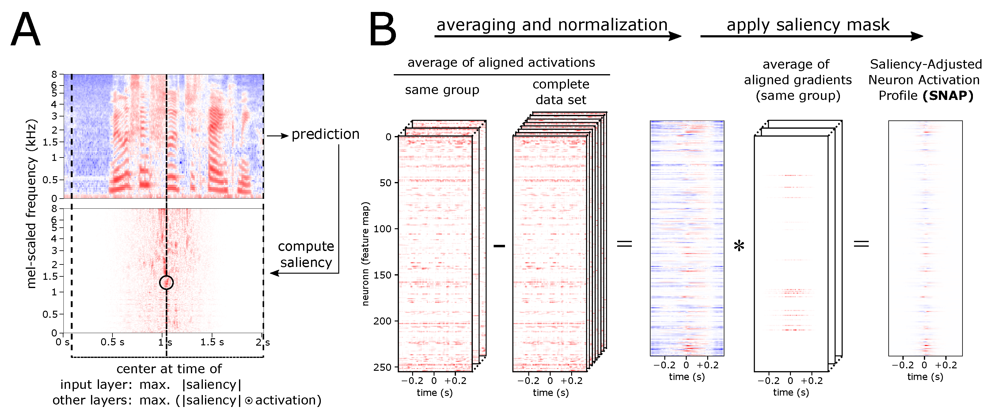
3.1. Normalized Averaging of Aligned Inputs (NAvAI)

We proposed NAvAI [8] as an adaptation of the ERP technique to ANNs. This method aims to reveal features in the input that are consistent across the group examples by averaging over inputs of the same group. We particularly evaluated NAvAI using the predicted letter as grouping. To properly apply an averaging approach, it is necessary that the input examples are temporally aligned. The reason is the same as for aligning different recordings at the same stimulus in ERP analysis: Without temporal alignment, relevant information is located at different times and hence removed when computing an average of the recordings. NAvAI follows the assumption that the predicted letter occurs in the recording at the time at which the input influences the network prediction the most. Correspondingly, NAvAI implements the alignment by centering the input spectrograms at the time of highest importance for the prediction, measured using the saliency map technique sensitivity analysis [26]. Specifically, the gradient of the logit of the predicted output unit with respect to the input values is computed as saliency map. NAvAI uses the information from sensitivity analysis only for the alignment step and only focuses on the input. SNAPs extend NAvAI by generalizing the alignment to the hidden layers of ANNs (see Section 3.3 for details). On top of that, we improve the alignment procedure by incorporating activation intensity and by reducing noise effects in the saliency maps. Furthermore, we incorporate information about prediction relevance from sensitivity analysis in the resulting SNAPs.

3.2. Neuron Activation Profile (NAPs)

We introduced the concept of NAPs in Krug et al. [9]. NAPs apply the normalized averaging procedure used in NAvAI to hidden layers of ANNs. However, in contrast to the inputs in NAvAI, feature maps in hidden layers are not aligned. Instead of using alignment, time-independence in NAPs is created by sorting the resulting averages per feature map on the time axis. This way, NAPs describe whether and how strongly each convolutional filter is activated for a particular group of inputs, but ignore the time of activation. While this simple method of creating time-independence is sufficient to compare NAPs of different groups, it neglects the temporal information that is necessary to accurately characterize feature maps in a more general context. Therefore, before averaging, our extension to SNAPs (see Section 3.3 for details) applies the alignment process from NAvAI to the feature maps in the hidden layers, as well. Moreover, taking the importance for the prediction into account is another advantage of SNAPs over NAPs.

3.3. Saliency-Adjusted Neuron Activation Profile (SNAPs)

The computation of the saliency maps used in SNAPs requires a prediction target. However, speech recognition is a transcription task, where the target output is a sequence of characters. In particular, before decoding, the output of our acoustic model is a sequence of $\lfloor t/2\rfloor$ vectors of class logits for an input of t time steps. The output has half as many time steps as the input because the initial convolutional layer is applied with a stride of 2. To compute a saliency map, we only consider the output of the model at a single time step, as if it was a classification. However, a single output time step only receives information from a part of the input corresponding to its receptive field. Therefore, using a complete input example is computationally wasteful. Instead, we split the whole input spectrogram into frames of a length equal to the receptive field size. These spectrogram frames of length $t_{rf}$ as inputs result in a sequence of $t_{out}=\lfloor t_{rf}/2\rfloor$ logit vectors. The model output for one such spectrogram frame has exactly one time step which is computed using the entire input. This time step is always in the center of the output sequence. Therefore, we use the corresponding output logit vector at $t_{target}=\lfloor t_{out}/2\rfloor$ for computation of the saliency maps.

In the first step of computing SNAPs, we center the activations of each layer and the spectrogram frames at the time of highest importance for the prediction. We refer to this step as “alignment” (Figure 1A). For the alignment, we consider activation values as important for a prediction if they have a strong activation with a high absolute sensitivity value. Therefore, we first derive neuron activations and sensitivity values in every layer for each spectrogram frame. Activation values are straight-forward to obtain from the forward pass through the network layers. To obtain sensitivity values, we compute the gradient of the (pre-softmax) logit of the highest active output unit in the center with respect to the activations of each layer.

Sensitivity analysis can result in single high gradient values at positions, where gradients of directly neighboring values are significantly smaller. This results from the independent treatment of input values during the gradient computation. To prevent that the alignment undesirably picks up these potential artifacts, we decrease the values of isolated high gradients. Because locating and decreasing them individually is computationally expensive, we instead apply average pooling with a $2\times 2$ kernel and stride 1 to the complete saliency map. This pooling operation averages adjacent values and hence decreases isolated high gradient values. At the same time, the small kernel size is applying only small changes to the values that are similar to their neighboring values. This average pooling is only used in the alignment step.

Finally, we align the activations by centering them at the time point of maximum $\left(\right|\mathrm{saliency}|\odot \mathrm{activation})$. The centering is implemented by cropping from one side and zero-padding the opposite side. Equivalently, we center the saliency maps so that they remain aligned to the activations.

Figure 1B visualizes the second part of obtaining a SNAP in a layer. First, we compute a group-specific profile by averaging the aligned activations that are obtained in the first step over a group of inputs. As some neurons show activations that are common to all inputs, we normalize the averaging result of each group by subtracting the average over the complete data set. Secondly, we similarly compute averaged aligned saliency maps for each group. However, we normalize saliency maps differently than activations to prevent that saliency values of zero lose their meaning. Instead of subtracting a global average, we scale averaged saliency maps to a range of $[0,1]$. Finally, we multiply the averaged and scaled saliency map with the normalized averaged activations to obtain a SNAP. This final step can be interpreted as masking information that is irrelevant for the prediction.

In addition, SNAP computation takes the particularities of the input and output layers into account. Input layer SNAPs are computed using spectrogram frames instead of activations. For SNAPs in the output layer, we use the logits instead of the softmax output. Otherwise, it can happen that SNAPs are vectors in which only the neuron for the predicted class is active (output value 1) and all others are not (output value 0). The distance between any pair of these vectors is the same, hence provides no informative distance for comparing the groups. This renders them useless for further analyses, for example the representational similarity analysis with clustering (Section 4.3.3). We observed this issue in our previous work [9] where we used softmax output values and obtained letter NAPs in the output layer with almost identical pairwise distances.

4. Experimental Setup

4.1. Data

ASR is typically evaluated with benchmark data sets like the LibriSpeech corpus [46]. However, this data set does not contain phoneme annotation, which limits the analysis to investigating the letter prediction. This is not optimal because letters in texts are often ambiguous as to how they are pronounced. In our previous work [9], we addressed this issue by obtaining a phoneme mapping through a letter-to-phoneme translation model. This mapping transcribed words to phonemes, which allowed analyzing how the letter prediction model responds to phonemes. Still, it was not possible to compare the predicted letters with a ground truth occurrence of phonemes in the speech recording.

For an in-depth analysis of our method, we require a data set which already provides annotation of the phonemes in the input data. Therefore, to be able to perform this kind of analysis in this work, we are training our models on the TIMIT data set [47] because it provides phoneme annotations. TIMIT is a small speech corpus in English language, containing 6300 speech recordings. Each of the 630 speakers recorded 10 out of 2345 unique sentences, but the distribution of how often each sentence was recorded is not uniform. In particular, TIMIT includes two sentences which are recorded for each of the 630 speakers, causing these sentences to be massively overrepresented. TIMIT refers to them as dialect (SA) sentences. To avoid overfitting on these instances, we only keep 7 random SA sentence recordings for training, corresponding to the number of speakers for each recording of the set of compact (CX) sentences. The models are trained using the provided data split, but excluding the majority of the SA instances. For the SNAP analyses, we use available examples from both the training and test data.

The letter transcriptions are readily available for training letter prediction models. Because the training of our model does not require targets for each time step, we can use texts as targets without mapping the letters to time steps. To obtain phoneme prediction targets, we need to adapt the provided phoneme annotations in TIMIT. These annotations provide a mapping of phonemes to time steps as a sequence of phonemes and their duration until the spoken phoneme changes. To convert this annotation into a target which can be used with the loss function of our model, we discard the information about the exact time duration and only use the phoneme sequences as transcription targets. Due to the small number of examples and speakers in TIMIT, the models trained on this data set do not generalize well in terms of ASR performance. However, this is no limitation for this work because we do not aim for high speech recognition capability but for demonstrating and evaluating our model introspection technique.

All data are preprocessed to mel-scaled log power spectrograms using the librosa library [48] using a FFT window size of 512 (32 ms) and hop size of 128 (8 ms) at 16 kHz and projecting the FFT bins to 128 mel-frequency bins. We do not normalize the spectrograms because our architecture comprises an initial batch normalization layer. For SNAP analyses, we split the spectrograms into frames of 206 steps (2 s) corresponding to the receptive field size of the model, that is, the time frame which the model uses for a single prediction. This results in about 330,000 spectrogram frames.

4.2. Model

We are using a fully-convolutional architecture to demonstrate our method. This architecture is based on Wav2Letter (W2L) by Collobert et al. [49], which is a 1D-convolutional architecture consisting of 11 layers, trained using the Connectionist Temporal Classification (CTC) loss [50]. This model can transcribe variable-length inputs of speech recordings to sequences of characters.

In this work, we train the model using the TIMIT data set [47] to transcribe speech as spectrogram to sequences of letters or phonemes. Furthermore, we made a few changes to the original architecture. As one adaptation, we changed the number of convolution filters in each layer to the closest power of two to improve computation efficiency on graphics cards [51]. Another difference to the original W2L model is that our architecture comprises one layer more in the stack of layers 2–9. We added one layer because a total of 12 layers allows for arranging information about all layers on a $2\times 6$ or $3\times 4$ grid. Although we do not make use of this property in this work, it makes the architecture a more convenient exemplary architecture for demonstrating visualization results. The parameters of the convolutional layers of the W2L architecture according to our adaptations are shown in

Table 1. Overview of parameters of 1D-convolutional layers in the used models.

Model Name	Layer	#Convolution Filters	Kernel Size	Stride
	1	256	48	2
W2L	2–9	256	7	1
W2L_TL_frozen	10	2048	32	1
W2L_TL_finetuned	11	2048	1	1
	(output) 12	29	1	1
W2P	1	256	48	2
	2–9	256	7	1
	10	2048	32	1
	11	2048	1	1
	(output) 12	62	1	1
	1	256	48	2
W2P_shallow	2–5	256	7	1
	(output) 6	62	1	1

. Before each convolutional layer, we use a batch normalization layer. In all layers except the output layer, we use ReLU as activation function.

In this work, we focus on analyzing how an ANN-based acoustic model processes speech. Accordingly, we do not use a subsequent language model because it would be independent of the acoustic model.

Model Variations

For our experiments, we use five different variations of the W2L architecture. The used parameters for the convolutional layers of all models are provided in Table 1. A summarized overview of all models used in this work is shown in

Table 2. Overview of models and which experiments they are used in. AE: Alignment Evaluation (Section 5.1), PS: Plotting SNAPs (Section 5.2), RS: Representational Similarity (Section 5.3), LP: comparing letter and phoneme representations (Section 5.4).

Model Name	#Layers	Output Type	Initializing Weights Using Model	Used in Experiments
W2L	12	letters	none	PS, RS, LP
W2P	12	phonemes	none	AE
W2P_shallow	6	phonemes	none	AE
W2L_TL_frozen	12	letters	W2P_shallow	RS
W2L_TL_finetuned	12	letters	W2L_TL_frozen	RS

at the end of this section.

The W2L architecture for letter prediction is our reference model. In our experiments, we continue to refer to the trained model as W2L.

For alignment evaluation (Section 5.1), we use W2L-based models that predict phonemes. One model is identical to the original architecture, but predicting phonemes. Accordingly, this model uses 62 output units in the output layer. We refer to this model as Wav2Phoneme (W2P). As we expect phoneme prediction to be an easier task than letter prediction, we also expect a model with fewer layers to be capable of performing this task. Therefore, we use a second phoneme prediction model that comprises only five convolutional layers and a final phoneme prediction layer, which we refer to as W2P_shallow. The used parameters of the convolutional layers are identical to the corresponding layers in the complete W2L architecture. We train both phoneme prediction models using the transcriptions generated from TIMIT phoneme annotations.

For evaluating experiments on representational similarity (Section 5.3), we train models such that there is an expected layer in which phonemes are best represented. To this end, we first train the W2P_shallow model to predict phonemes. From this model, we remove the final phoneme prediction layer (layer 6). On top of the pre-trained layers, we add layers to form the W2L model again, using letters as output. This approach of training a model and using its parameters to initialize all or some layers of another model is referred to as transfer learning. In the first step of transfer learning, we only train the added layers by disabling parameter updates of the pre-trained layers. As disabling parameter updates is commonly referred to as freezing, we call the resulting model W2L_TL_frozen. In the W2L_TL_frozen model, we expect the base layers to encode phonemes, while the top layers learn to map from the phoneme representation to letters. In the second transfer learning step, we unfreeze the base layers and perform a fine-tuning over all layers (W2L_TL_finetuned). Note that we do not fine-tune the batch normalization layers as this can lead to unlearning the pre-training information. We use the W2L_TL_finetuned model to investigate to which extent the fine-tuning process changes the pre-trained phoneme encoding in favor of better prediction of letters.

4.3. Evaluation

Proper alignment is a crucial requirement for the averaging approach. Therefore, we first evaluate this step in more detail to ensure that our alignment approach is accurate. Secondly, we present two strategies to use SNAPs for getting insight into the model. This section describes how we perform these evaluations.

4.3.1. Evaluating the Alignment Step

From the TIMIT data set, we use the phoneme annotation of each time step for evaluating the accuracy of the alignment. Alignment is supposed to center inputs (or activations) such that, for a prediction, the center of the frame is set to the actual occurrence of the predicted phoneme in the input. We test this by comparing the predicted phoneme with the annotated phoneme at the alignment position. If the alignment is only wrong by a few time steps, the averaging is slightly blurred but not entirely wrong. Therefore, we additionally test whether the predicted phoneme is contained in a small time window of +/− two steps (corresponding to +/− 16 ms) around the alignment point. We quantify the quality of the alignment by its accuracy, that is, the fraction of input frames that are aligned to the correct phoneme (or window around it). For measuring the error of the alignment of one example, we compute the alignment offset as the distance of the alignment point to the target time step. Quantifying the alignment quality and offset is only possible for models that predict phonemes because there is no unique mapping from predicted letters to annotated phonemes. Therefore, we perform a quantitative evaluation using the phoneme prediction models W2P and W2P_shallow.

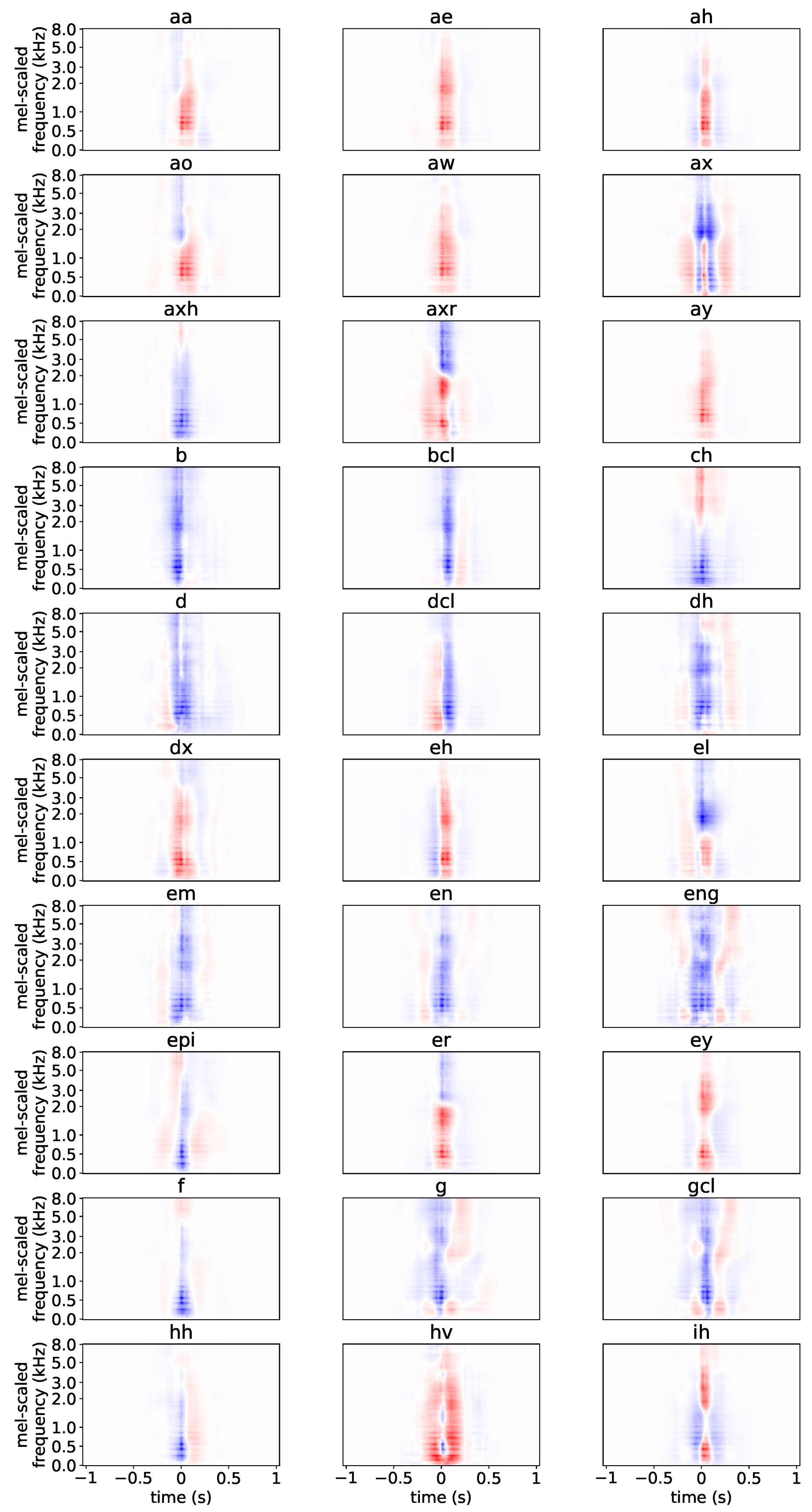
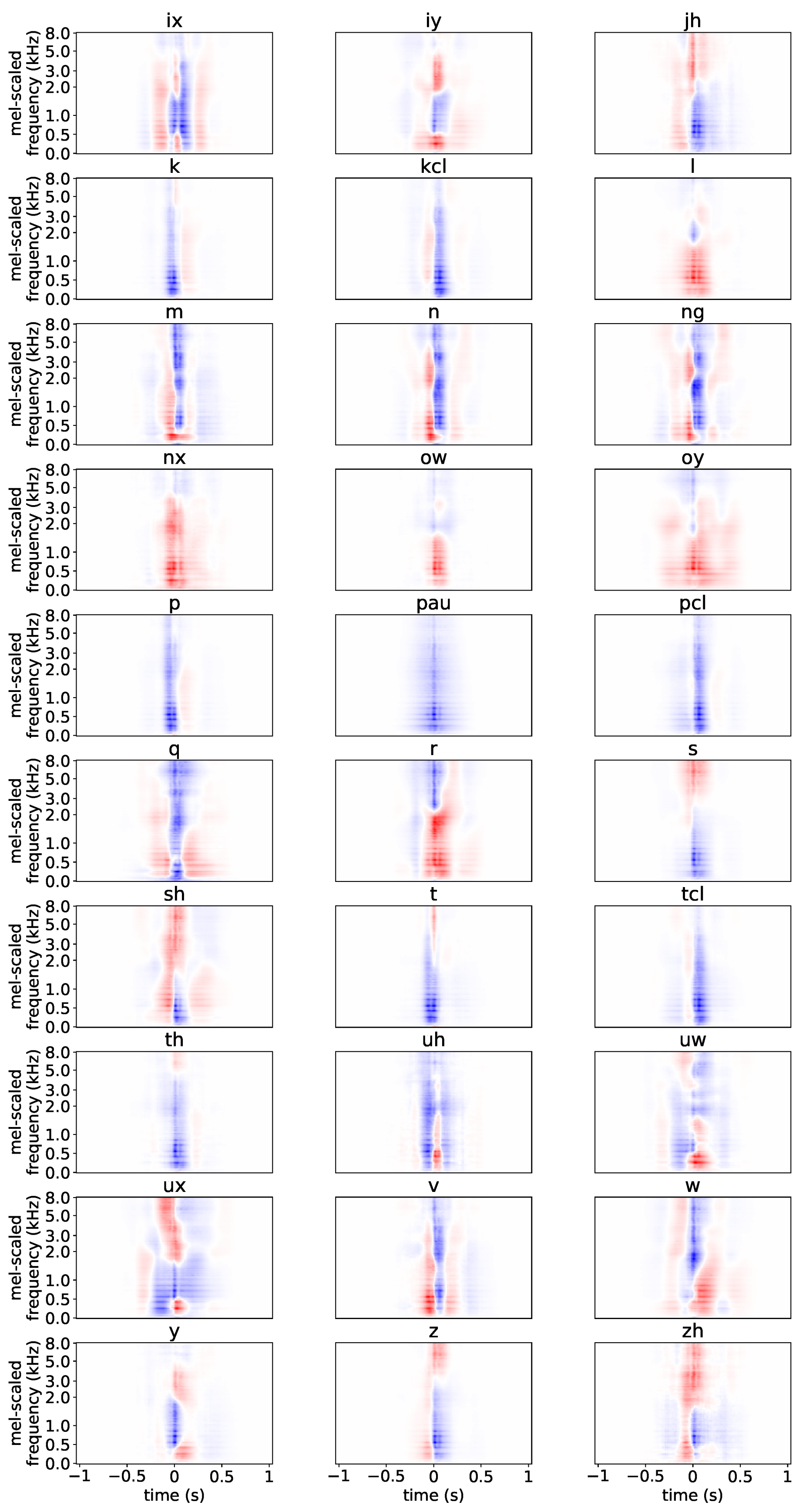
4.3.2. Plotting SNAPs

For data that are visually interpretable, input layer SNAPs are interpretable, as well. Although understanding spectrograms requires some domain knowledge, we consider them to be interpretable. However, due to the normalization, input layer SNAPs are not spectrograms but describe how the intensities of the frequencies for the represented group differ from the rest of the data. Plots of hidden layer SNAPs are interpretable in fewer cases because it requires that the hidden layer activations can be interpreted themselves. To a certain extent, this is possible for 2D-CNNs applied on visually interpretable data. In such case, SNAPs that correspond to single feature maps can be plotted and inspected. In the 1D-CNN that we use in this work, feature maps are only one-dimensional and, in contrast to the frequency dimension in the input, do not have a meaningful ordering. In a one-dimensional case, inspecting the SNAP values is possible by plotting them as line plots, where each feature map corresponds to one line. Our used models have hundreds of one-dimensional feature maps per layer, which leads to correspondingly many different lines in the line plot. Therefore, this visualization is difficult to interpret for our specific model. Hence, in this work, we demonstrate visual inspection of SNAPs only for the input layer.

We use the W2L model to evaluate visualizations of input layer SNAPs. To this end, we first compare input layer SNAPs of letters with NAvAI results to show the advantage of using saliency map information. Secondly, we evaluate whether SNAPs of phonemes reveal representative patterns by qualitatively comparing exemplary input layer SNAPs with expected phoneme-typical patterns.

4.3.3. Representation Power of Layers for Different Groups

We applied hierarchical clustering with Euclidean distance and complete linkage [52] to NAPs of letters and phonemes in our previous work [9], using a fixed threshold for the emergence of clusters. Here, we investigate the clustering approach using different distance thresholds at percentiles 87% to 96% in steps of 3%. We empirically found these thresholds to lead to different numbers of clusters for our model. Applying the clustering algorithm to other models might need other thresholds if distance value range or distribution are different due to model properties, for example the used activation function. For quantifying the quality of the clustering result, we compute its Silhouette score [53]. The Silhouette score is a measure of how similar instances in the same cluster are to each other compared to their similarity to instances of the nearest other cluster. In the context of SNAPs, a high clustering quality in terms of Silhouette score indicates that the set of observed groups is separable into disjunct subsets, such that groups in the same set activate neurons similarly and groups of different sets activate neurons differently. The resulting subsets are potential high-level concepts that the network learned to encode in the respective layer. However, high clustering quality does not guarantee that this concept is meaningful to human interpretation. Therefore, evaluating whether the clusters are interpretable subsets of groups still requires to manually inspect the clusters. In addition to investigating the Silhouette scores at individual distance thresholds, we further investigate the average Silhouette score over the four used thresholds in each layer.

We evaluate this approach by contrasting the W2L model with the models that we trained by applying transfer learning (compare Section 4.2). Through transfer learning, the five bottom layers of the models W2L_TL_frozen and W2L_TL_finetuned are pre-trained to predict phonemes. Therefore, we expect the best clustering of phonemes to emerge at this depth of the networks and to be better than in the W2L model. This expectation is independent of whether the clusters correspond to interpretable concepts like phonemic categories. Furthermore, for the W2L model, we compare the clustering of SNAPs between grouping by predicted letter and annotated phoneme.

5. Results

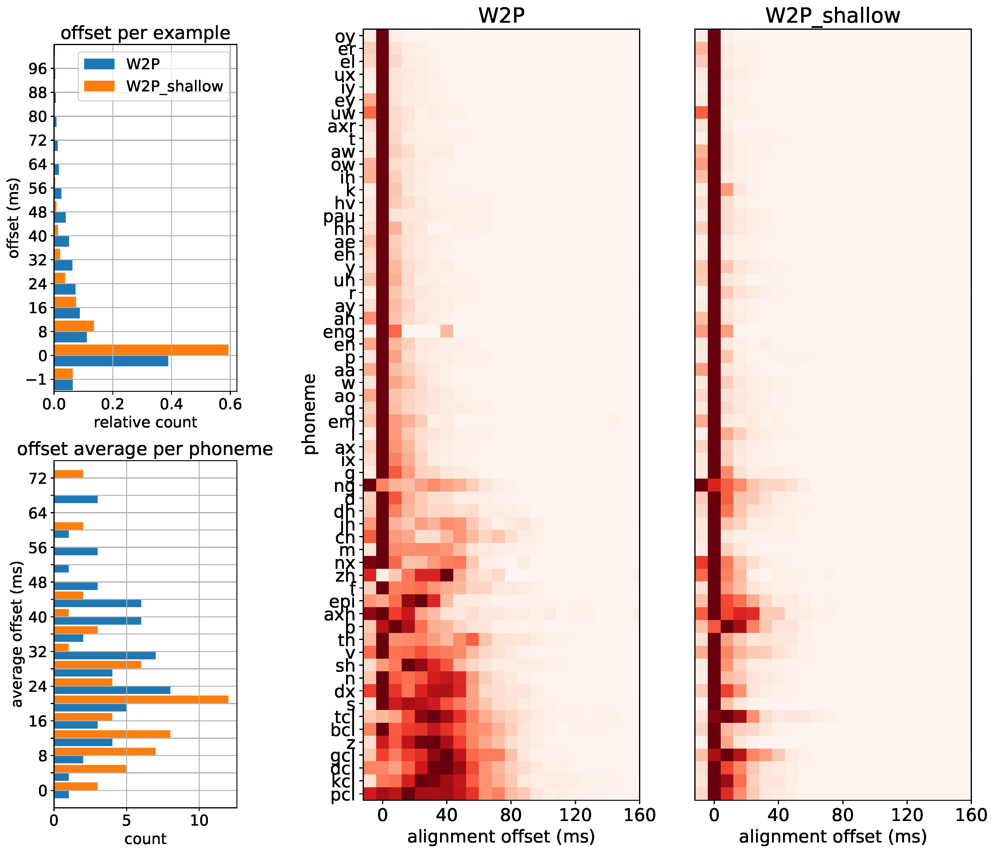
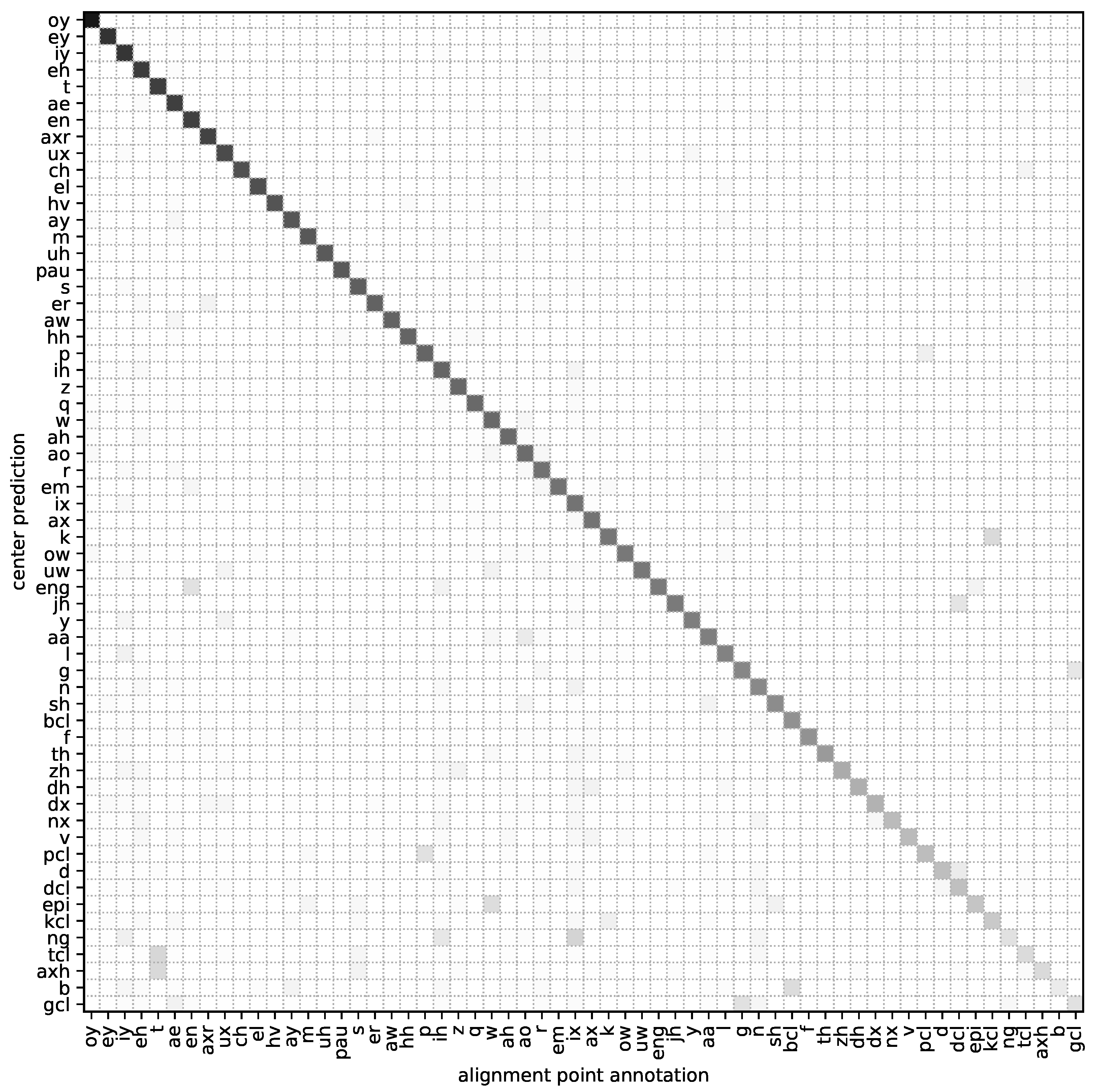
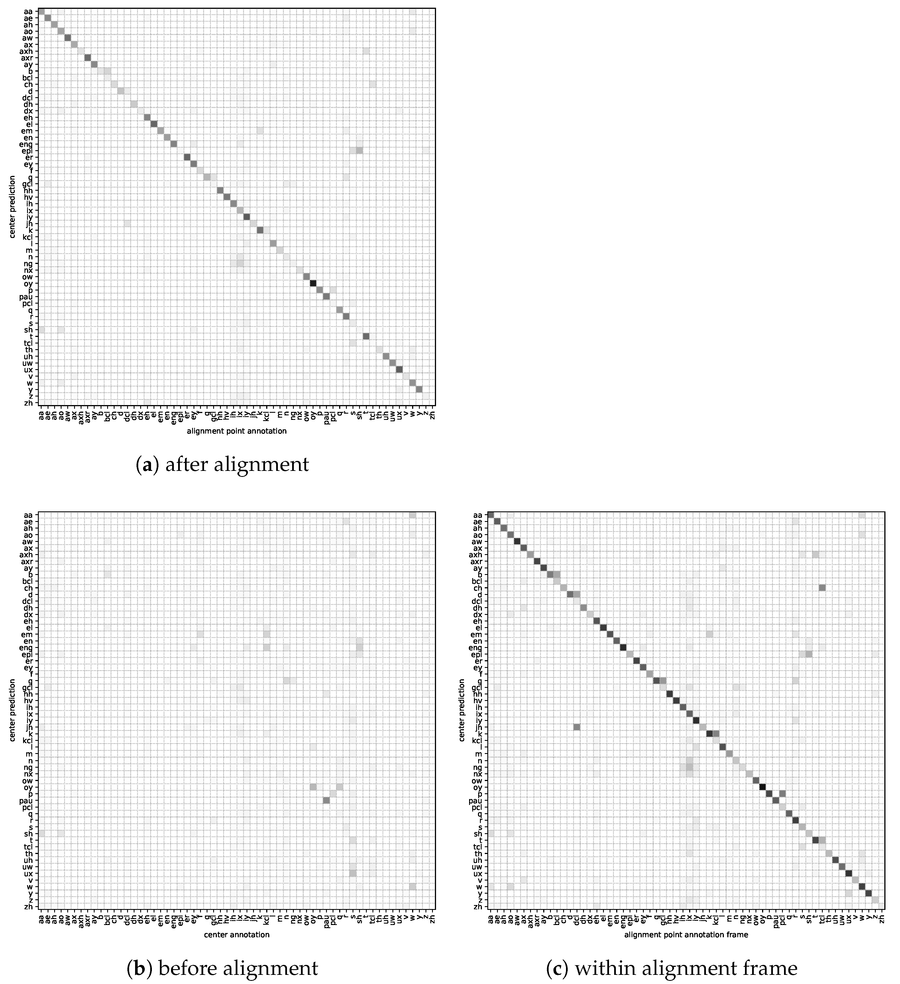
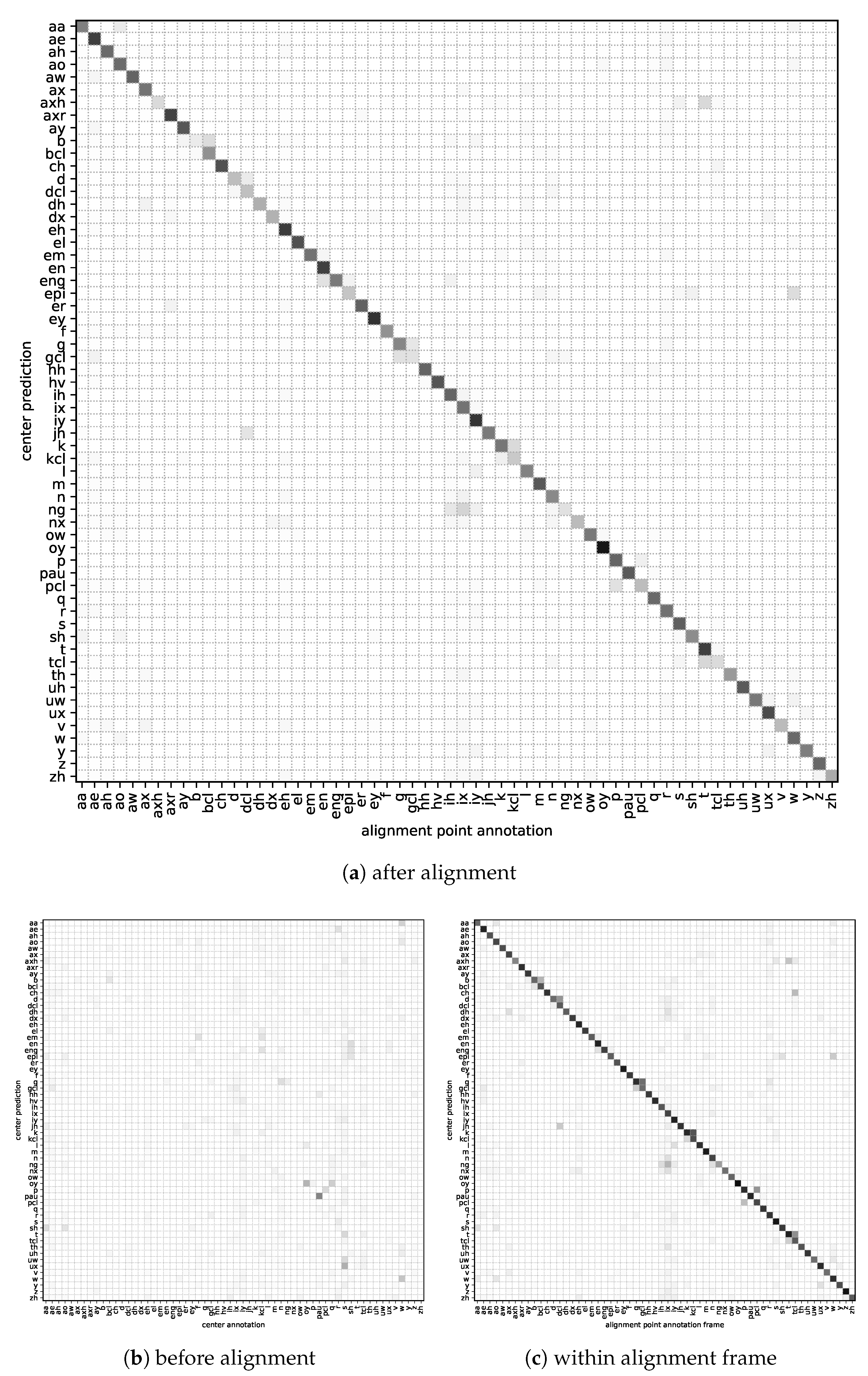
5.1. Alignment Evaluation

To evaluate the alignment step of the SNAP computation procedure, we use the two models that predict phonemes: W2P and W2P_shallow (compare Section 4.2). We expect our method to align at the time steps in the input spectrogram frame which are the actual occurrences of the predicted phonemes. Therefore, for each prediction, we additionally obtain the annotated phoneme at the center and the alignment position. Moreover, we compute the time difference of the alignment position to the real occurrence of the predicted phoneme according to the annotation. We then use this distance to quantify the alignment error and refer to this measure as “alignment offset”. For instances that are predicted as a phoneme which is not contained in the annotation of the input spectrogram frame, we define the alignment offset to be −1. Because the alignment cannot be correct in these cases, the maximum possible alignment quality for our data set and both phoneme prediction models is to align 93.6% of the instances correctly.

5.1.1. Alignment Quality—Model Average

W2P_shallow: Initially, only 3.7% of the frames are annotated with the predicted phoneme in the center. Through alignment, this can be observed for 59.3% of the frames. Allowing an alignment offset of up to two time steps (16 ms), the predicted phoneme is equal to the annotated one for 80.3% of the frames. For the W2P_shallow model, we observed an average alignment offset of 26 ms.

W2P: Only 3.6% of the frames are matching prediction and annotation at the center time step. Alignment increased this number to 38.8%. Considering also the annotated phonemes in a time frame around the alignment point, 58.6% of the frames were correctly aligned. Corresponding to the smaller alignment accuracy than the W2P_shallow model, we also observe a higher average offset of 37 ms in the W2P model.

For the two phoneme prediction models, we conclude that our alignment method works as expected in a large number of frames. Because the averaging takes all instances into account, it is sufficient to align the majority of the frames correctly. Notably, the deeper model for phoneme prediction has a significantly worse alignment accuracy than the shallower model. We suspect that this related to an overfitting of the deep model on the training data. An overfitted model is not learning meaningful features but memorizes information, which allows it to perform correct predictions without focusing on the actual occurrence of the sound. Hence, for the W2P model, we argue that the alignment works properly despite the lower accuracy. The provided alignment accuracy metric for the phoneme models is computed as average over all phonemes, yet there are substantial differences between them. Therefore, we further investigate the alignment accuracy and offset for each individual phoneme.

5.1.2. Alignment Quality—Per Phoneme

Figure 2, in the center and right columns, shows the per-phoneme alignment offset distributions for the two investigated models. The rows are sorted by the average alignment offset of the corresponding phoneme in the W2P model.

We generally observe larger offsets for W2P than for W2P_shallow corresponding to the average alignment offset of the models.

For W2P, 25 out of 60 phonemes are aligned without offset in the majority of instances. Six out of the seven phonemes of highest alignment offset are closure symbols (pcl, kcl, dcl, gcl, bcl, tcl), describing the closure of plosives. For example, pcl represents the closure of p. Because the W2P model has a higher capacity and a larger receptive field than the W2P_shallow model, it might predict phonemes by finding correlations to other phonemes. Especially for the closure symbols, we intuitively expect that the model might facilitate that they always precede the corresponding plosive. However, by manually inspecting the most frequent phonemes at the alignment point, we do not observe this behavior. We also did not find any other intuitively interpretable correlation which the model grasped.

In the smaller W2P_shallow model, 44 phonemes are correctly aligned in the majority of instances. A smaller alignment offset is also observed for all closure symbols. More specifically, all closure symbols except for gcl and tcl are aligned without error in most of the instances.

These observations support further that the decreased alignment performance for the W2P model is not attributed to our alignment technique but to the worse generalization capabilities of the model. Moreover, this contributes to considering the W2P_shallow model as being easier interpretable than the W2P model.

In addition to the alignment offset, we also investigate in more detail, which annotated phonemes the predicted phonemes are aligned to. In this section, we provide detailed plots only for W2P_shallow because it generalizes better than the W2P model. An overview of the evaluation plots for both models using alphabetical ordering of phonemes is provided in the Appendix A in Figure A1 and Figure A2. For the W2P_shallow model, we show the complete contingency table in Figure 3, for the predicted phoneme and the annotated phoneme after alignment. To get a better impression of how consistently which phonemes are aligned to a specific phoneme, we sort the table by the maximum value per row. We do not observe a clear tendency of a specific type of phoneme being better aligned than others. Moreover, the closure symbols are still aligned to various other phonemes, although the effect is not as pronounced as in the W2P and vanishes when allowing a small alignment offset.

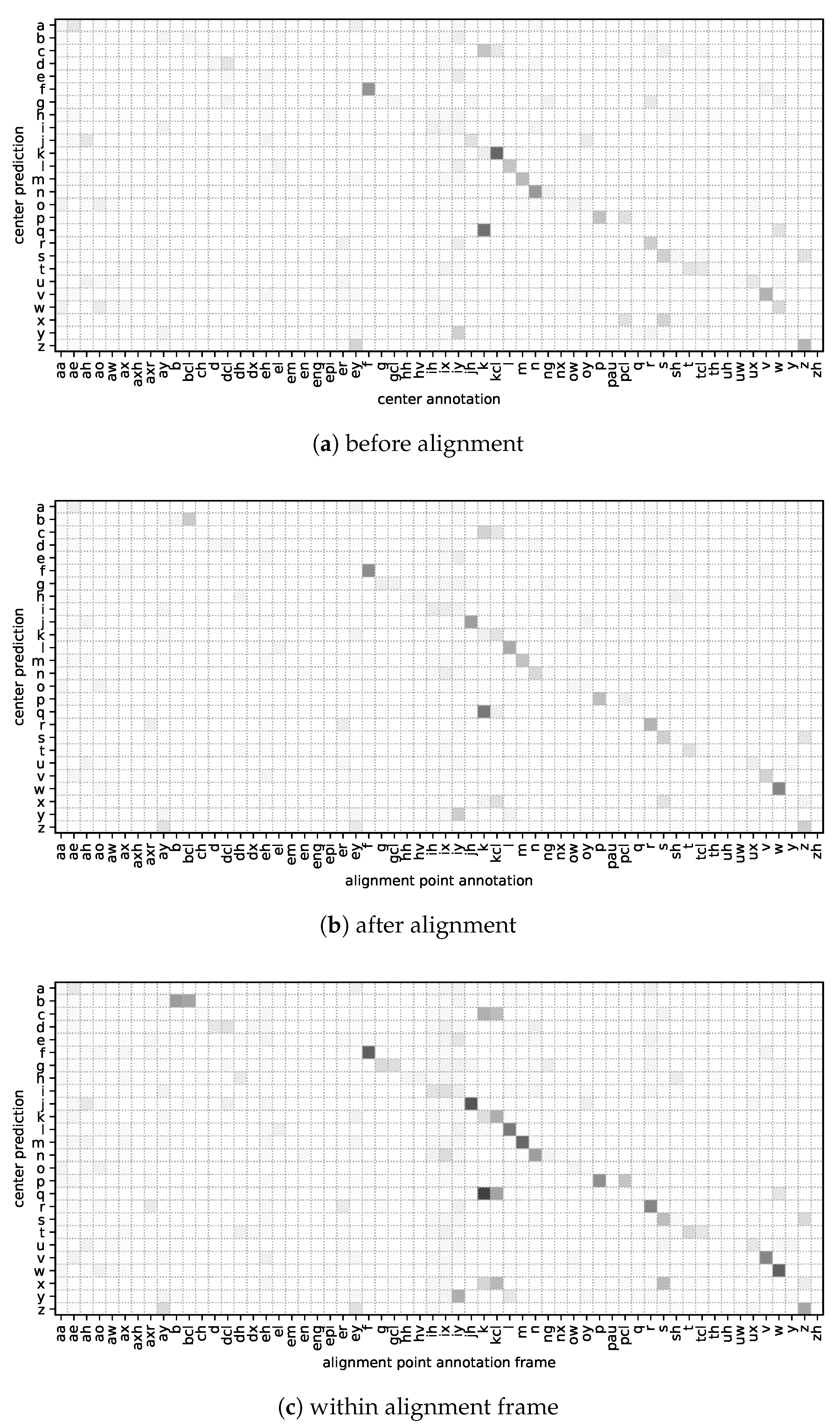
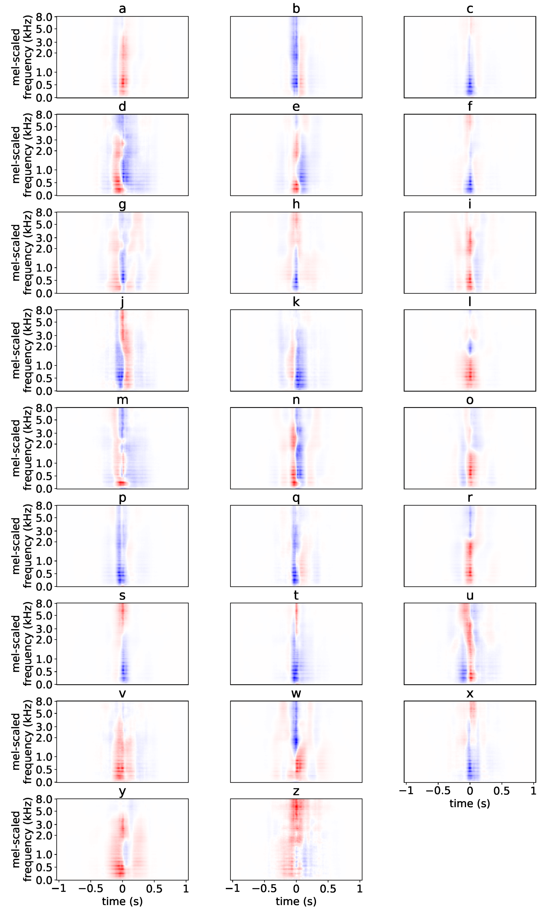
5.1.3. Applicability to Letter Prediction Models

As discussed before, performing the same quantitative analysis for a letter prediction model is not possible. There is no unique mapping from letters to the phonemes, so we cannot test for equality of prediction and annotation. Moreover, a predicted letter can be correctly aligned to different phonemes, which leads to less specific alignment results than in the phoneme prediction models. Still, we can use the phoneme annotation to investigate which phonemes the predicted letters are aligned to. The contingency tables for W2L are shown in the Appendix A in Figure A3. Qualitatively, the alignment improves how well the annotated phoneme at the center position corresponds to the predicted letter. For example, without alignment, spectrogram frames that are predicted as letter b are very rarely annotated with the phonemes b or bcl at the center time step. After alignment, the majority of the frames predicted as letter b is centered at these phonemes.

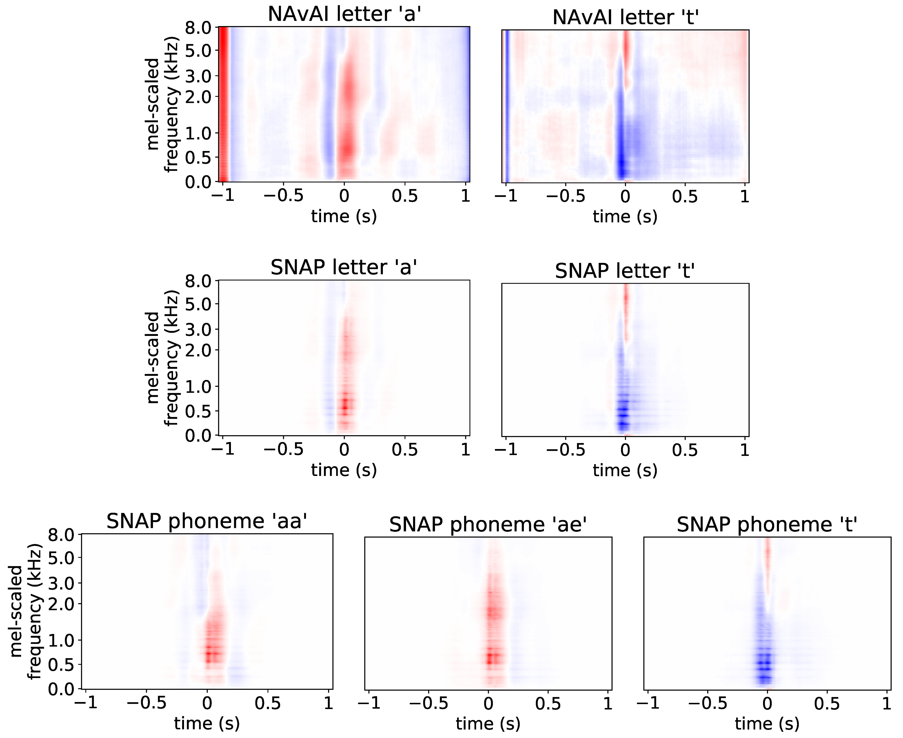
5.2. Per-Layer SNAPs

SNAPs in the input layerare an improvement of NAvAI [8]. Examples of SNAPs in the input layer compared to exemplary NAvAI results for W2L are shown in Figure 4.

Input layer SNAPs are directly interpretable. They show how the intensity of frequencies differs from the average over the complete data set, indicated with red and blue color for higher and lower intensity, respectively. The gradient-based masking guarantees that the SNAPs only show regions which are important for the prediction. This advantage over NAvAI is demonstrated comparing the top and middle row in Figure 4. While NAvAI shows a pattern over the whole receptive field size, the corresponding SNAP also identified prediction-relevant parts of the pattern. In addition to providing more information about what part of the input the model uses for prediction, SNAPs implicitly mask the padding artifacts that occur in NAvAI as a result from the alignment procedure. An example for these padding artifacts are the high values at −1 s in the NAvAI pattern of letter a.

We observe phoneme-typical patterns in the input layer SNAPs (Figure 4 bottom). Phonemes aa and ae share a high intensity formant at around 700 Hz. A second formant is identified at around 1200 Hz and 1900 Hz for aa and ae, respectively. The input pattern for t shows a change of high to low intensities of all frequencies at the alignment time. The patterns for all three observed phonemes match the expectation well. A main difference is that identified formants are spreading a wider range of frequencies, which is an expected effect when averaging recordings of different speakers.

The NAvAI and SNAP results for letter a are more similar to the input layer SNAP for phoneme ae than to the SNAP for phoneme aa. This indicates that letter a was pronounced as ae more frequently than as aa and furthermore demonstrates how the SNAP of letter a is dominated by the over-represented pronunciation ae. This dominating effect can happen for groups with high variation between the instances. Therefore, it particularly affects unbalanced groups in which a subset of instances is more homogeneous than the other instances. Because of this, SNAPs are best suitable for groups with small intra-group variance. Consequently, in this work, we compute SNAPs for individual phonemes, instead of using higher-level grouping like vowels or fricatives. Input layer SNAPs in model W2L are shown in the Appendix for all annotated phonemes in Figure A4 and Figure A5 and for predicted letters in Figure A6.

In deeper layers, feature map order is uninformative because there are no connections between feature maps in the same hidden layer. Therefore, the corresponding SNAPs cannot be interpreted by visual inspection. An example can be seen in Figure 1B (rightmost).

In all layers, we observe that SNAP values become smaller and drop to 0 the further away they are from the alignment time. This indicates that the model does not use the complete receptive field for the prediction of the majority of instances. Thus, it is possible to compress the model, for example by choosing fewer layers or filters or by decreasing the kernel sizes.

5.3. Evaluation of the Representational Similarity

We evaluate whether SNAP clustering can indicate representational quality. To this end, we first investigate Silhouette score correspondence to a ground truth obtained through transfer learning and, based on the findings, inspect the emerged clusters in specific layers. For this evaluation, we compare the three models W2L, W2L_TL_frozen and W2L_TL_finetuned (compare Section 4.2).

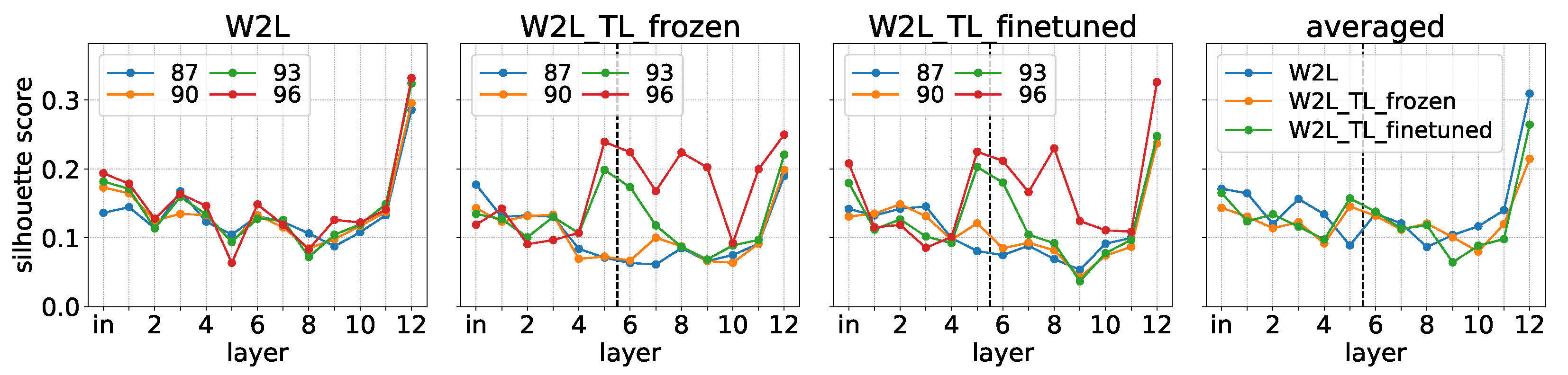
5.3.1. Silhouette Scores

Figure 5 shows an overview of the Silhouette scores for clusterings in all layers of the used models at different distance thresholds as well as averaged over all the used distance thresholds. In general, higher Silhouette scores indicate better clustering quality. By increasing the distance threshold, the number of clusters decreases.

Regarding the average Silhouette scores, the models do not differ substantially. We observe the highest difference between any two models in the output layer, where the W2L model had an average Silhouette score of 0.31 and the W2L_TL_frozen model only 0.21. The second largest difference is in layer 5, where the Silhouette score is higher for the TL models (frozen: 0.15, finetune: 0.16) than for the W2L model (0.09).

The non-averaged Silhouette score curves are more clearly distinguishable between the transfer learning models and the W2L model. Using smaller distance thresholds (87th and 90th percentile), the Silhouette scores are higher for the W2L model than for the transfer learning models, but the difference between the clustering qualities of the models varies between layers. However, for the W2L model, we do not observe a change in clustering quality when increasing the distance threshold. This is contrary to the transfer learning models, in which Silhouette scores increase strongly from layer 4 to 5 when using higher distance thresholds (93th and 96th percentile). At the same layer, the W2L model decreases in Silhouette score. We consider this a random co-occurrence because it is independent of our choice of the depth of the transfer learning base model.

We expected that phonemes are best represented in the fifth layer of the transfer learning models because it is the deepest layer of the ones that are pre-trained on phoneme prediction. For the higher distance thresholds, the Silhouette scores correspond to this encoding that is induced through pre-training. This demonstrates that clustering quality can be used to investigate representation of groups. However, the result is sensitive to the choice of parameters for the clustering algorithm. We therefore recommend not to rely on a single parameter setting but to perform the clustering evaluation with different parameters even though it multiplies the computation time.

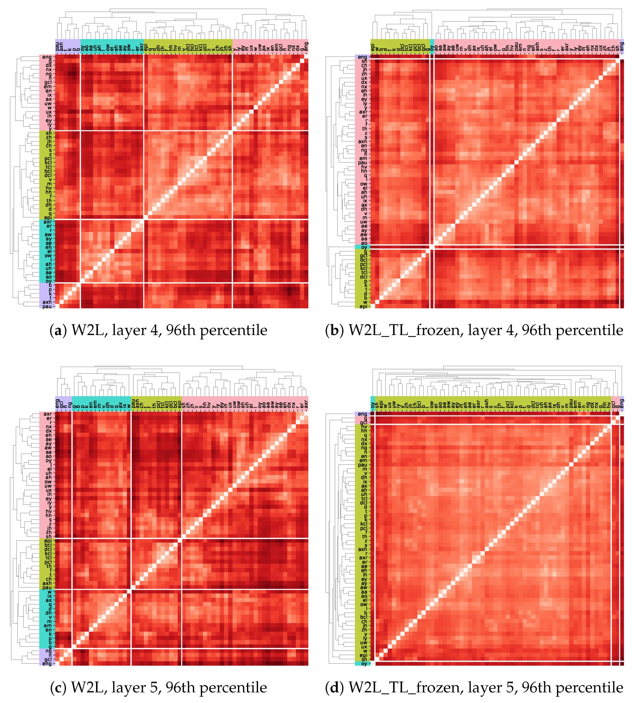
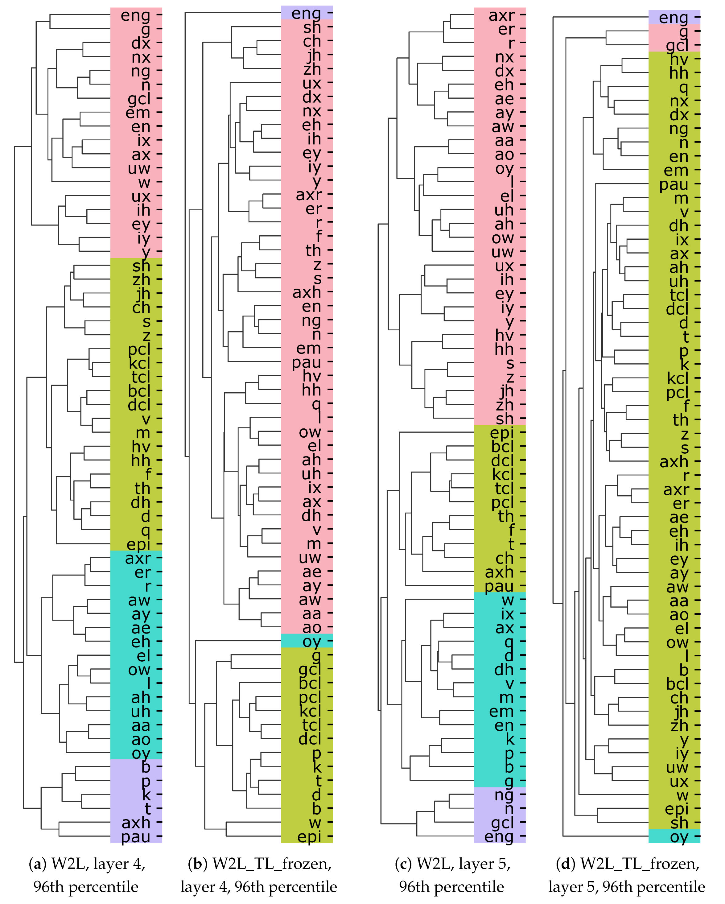
5.3.2. Emerged Clusters

In addition to only observing the Silhouette score as a metric, we investigate the emerged clusters in more detail. As described before, there is a high change in Silhouette score in both the W2L_TL models and the W2L model from layer 4 to 5, which is the highest for the clustering at the 96th percentile. Therefore, we investigate the clustering result at the 96th percentile threshold in layers 4 and 5 in more detail. As the frozen and finetuned model do not differ substantially, we only further compare W2L and W2L_TL_frozen. A visualization of the SNAP clustermaps is shown in Figure 6 and an enlarged view of the corresponding clustering assignments is shown in Figure 7. In the following, we will refer to clusters of at least three grouped phonemes as “main clusters” and focus on them because they indicate groups of similar representation.

For W2L_TL_frozen, two distinguishable main clusters emerge in layer 4, while in layer 5 there is only a single large cluster. Observing a single large cluster with high pairwise similarity values indicates good representation on the level of individual phonemes. Because the model distributes phonemes evenly in the representation space, it is able to distinguish between each of the individual phonemes. This is our expected result because the fifth layer of the W2L_TL_frozen model is the deepest layer that is pre-trained on phoneme prediction trough the transfer learning approach. Decreasing the clustering distance threshold in the transfer learning model forces the clustering to divide the homogeneous cluster, leading to significantly smaller Silhouette scores.

The W2L model, in contrast, showed more distinct subclusters in both the 4th and 5th layers. The number of clusters is the same in both layers but the sets of phonemes being assigned to the same cluster is substantially different. 35.4% of phoneme pairs change from being assigned to the same cluster to being in different clusters or vice versa. At the same time, distances between SNAP in the W2L model are much higher and vary more than in the transfer learning model. Phoneme clusters in the W2L model indicate that the model encodes high-level concepts of similar sounds. For example, the red cluster in the 5th layer (Figure 6c and Figure 7c) contains most vowels.

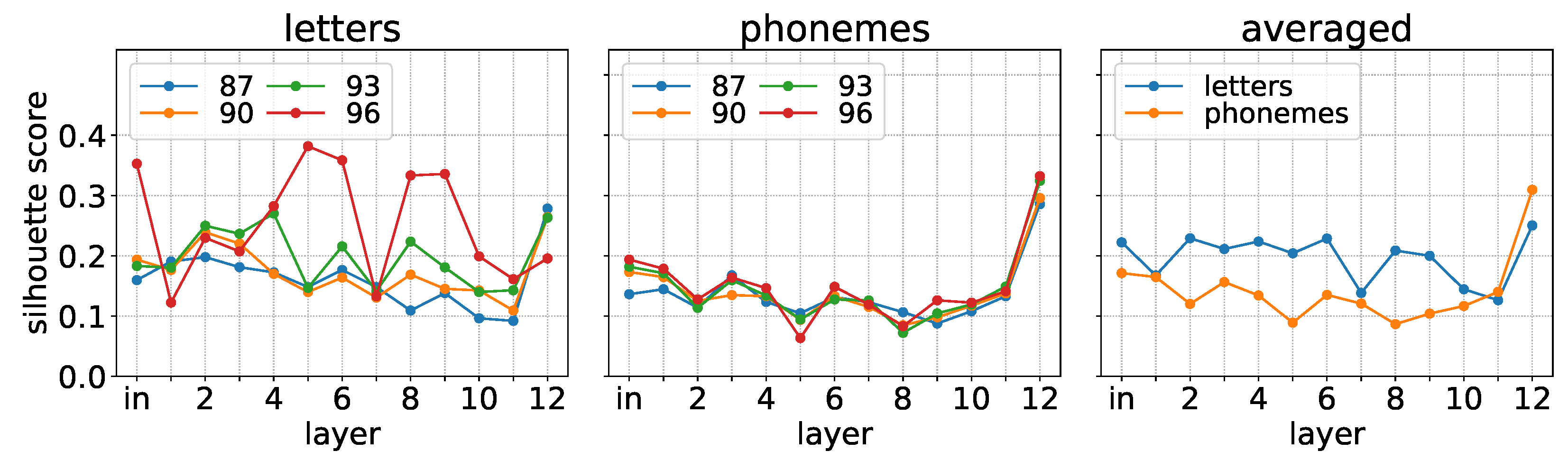
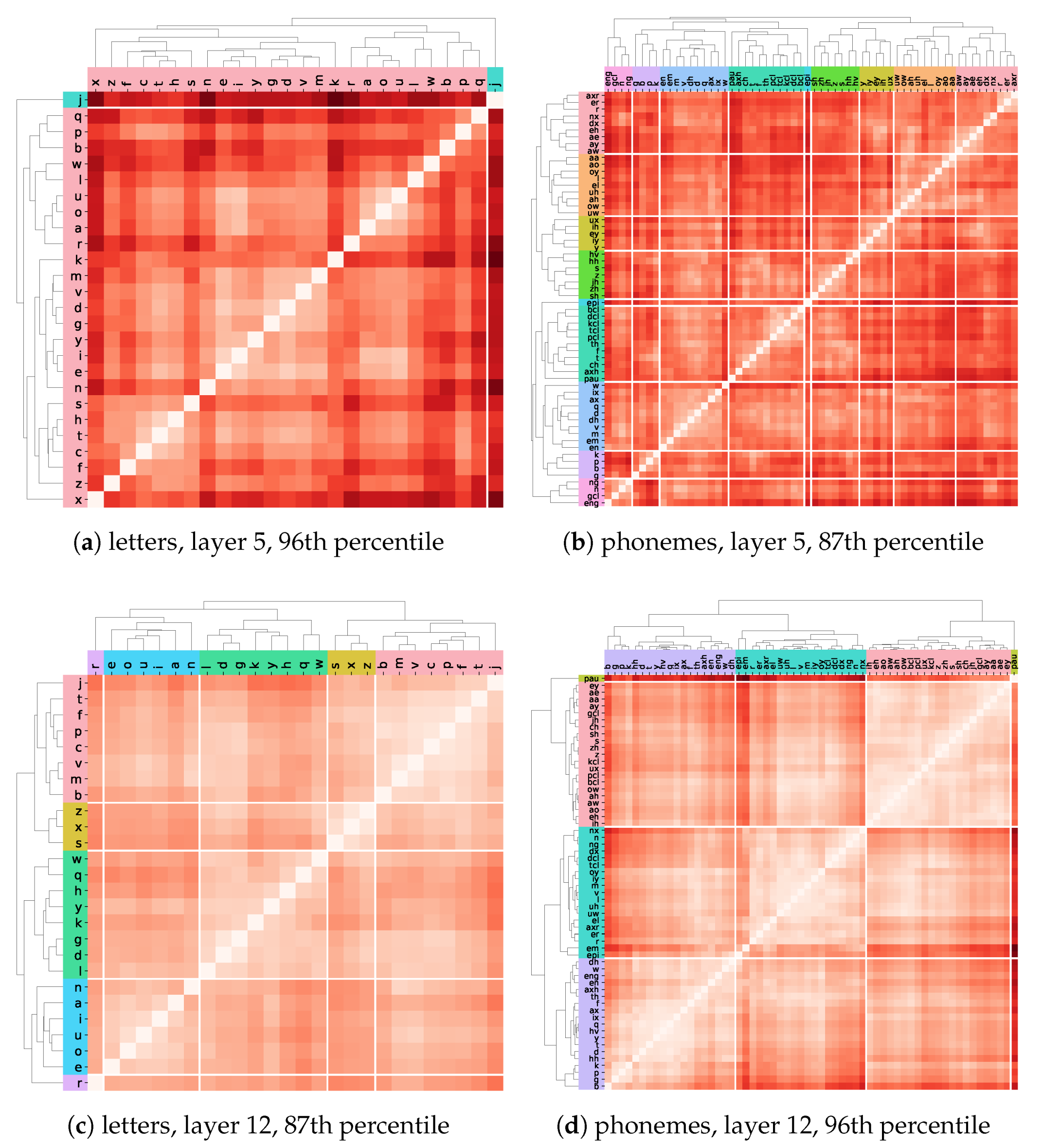
5.4. Comparing Letter and Phoneme Representations in W2L

To demonstrate an application of SNAP clustering, we investigate whether the W2L model implicitly encodes phonemes as intermediate representation for predicting letters. First, we compute SNAPs for the W2L model using phonemes and letters as grouping, respectively. Grouping by letter uses the predictions of the model and phoneme grouping is based on the annotated phonemes at the center time step of the input spectrogram frame. We then cluster both sets of SNAPs in each layer and compute the Silhouette scores at different distance thresholds. In the input layer, we cluster the spectrogram frames. Figure 8 shows the result for letters (left), phonemes (center) and the averages over distance thresholds for both groupings (right).

For letters, the clustering quality strongly depends on the chosen distance threshold, while the threshold has only minor influence on the phoneme clustering quality. Particularly, clustering at 96th percentile of letter SNAPs differs from clustering at smaller distance thresholds. Compared to the evaluation experiment in the previous Section 5.3, the observed Silhouette score curves are not as conclusive. According to the Silhouette scores, letters are clustered better than phonemes in all except the two final layers. This is surprising as we expect a letter prediction model to specifically cluster letters well in the output layer. Moreover, letter clustering has the highest Silhouette score in layer 5 (at 96th percentile), while phoneme clustering has its minimum clustering quality in this layer.

Because layers 5 and 12 stand out in terms of clustering quality, we investigate clustering in these layers in more detail. We particularly compare the SNAPs for letters and phonemes in the W2L model, using the respective distance threshold with the highest respective clustering quality. A detailed visualization of the pairwise distances between the SNAPs as clustermaps is shown in Figure 9, while Figure 10 shows the corresponding clustering assignments as enlarged view.

Although the Silhouette scores indicate better clustering for letters in layer 5, only a single-letter cluster for j is distinguishable from all other letters. In addition, several similarities are not reflecting interpretable concepts. For example, unexpectedly, letter r is most similar to letters a, o and u. We similarly observed a single large cluster for the transfer learning model in the evaluation experiment (Section 5.3, Figure 6d). The main difference is that the distance values between letter SNAPs are much higher than the distances between phoneme SNAPs. In this case, we suspect that the high clustering quality is an artifact from distinguishing the SNAP of j as the rarest group (only 160 frames are predicted as j). Emerging phoneme clusters in layer 5 are representing more meaningful groups, although having lower Silhouette score. The pink cluster encompasses nasals (ng, n, eng). Green contains multiple fricatives (s, z, zh, sh). Purple only consists of plosives (k, p, b, g). Red, orange and yellow are mainly grouping different similar sets of vowels (and semivowels).

In the output (12th) layer, we observe more meaningful clustering of letters, for example, a cluster containing all vowel letters and a cluster of sibilant-typical letters (blue and yellow cluster in Figure 9c, respectively). However, other letters that we expected to be close (for example, p and b or t and d) are far apart from each other. We hypothesize that this indicates how certain the model is when predicting particular letters. For example, p and b might be easy for the model to distinguish, which leads to output layer activations and corresponding SNAPs that are more distant from each other.

In the previous Section 5.3, we observed a similar pattern for the phoneme clustering in the fifth layer of the W2L_TL_frozen model (Figure 6d). There, we suspected that the W2L_TL_frozen model can easily distinguish between the phonemes in the fifth layer and therefore distributes them more evenly in the representation space. For letter prediction in the W2L model, however, it appears to be harder to distinguish between some of the letters, which leads to the corresponding output layer SNAPs being more similar to each other. We conclude that this difference of the clustering results between the models reflects that it is more difficult to distinguish between letters than phonemes, which is reasonable considering the high variability of how letters are pronounced.

For phonemes in layer 12, emerging clusters are more distinct from each other, both compared to the letter clustering as well as compared to phoneme clustering in layer 5. Phoneme pau as pause marker is clearly distinguishable from the other phonemes. Apart from that, we observe that the clustering of phoneme SNAPs in layer 12 is worse than in the fifth layer. The emerged clusters do not represent any phonemic category both in terms of their size and the phoneme similarities. This observation supports our expectation that phonemes are worse represented in deeper layers of the letter prediction model, in particular in the output layer. In addition, the phoneme SNAP clustering result demonstrates that there cannot be a strong correspondence between phonemes and letters. If there was such correspondence, a phoneme SNAP in the output layer would show high activations for a particular letter output neuron, hence show clustering behavior that is similar to the corresponding letter.

6. Conclusions

SNAPs are a promising tool to gain insight into ANNs. They combine strengths of existing introspection techniques, extend them and allow for more comprehensive analyses. With our method, introspection is not limited to the predicted classes but can be performed for any grouping of inputs. Moreover, model introspection is flexibly possible for different parts of the network, for example inputs, any layer or specific subsets of neurons.

In this work, we presented per-layer clustering of SNAPs for different groups and investigated Silhouette score to measure how well groups are represented. We found that observing the clustering quality alone cannot reveal layers which encode meaningful and interpretable concepts of particular groups. However, it helps to make an informed choice about which layers to inspect in more detail with additional introspection methods. Considering the increasing depth of modern ANNs, this already is a valuable aid in model analysis. A limitation of the clustering is that the visualization becomes cluttered if there are too many groups, which can be circumvented by choosing higher-level groups or a smaller subset of groups of interest.

Notably, computing SNAPs is generally possible for any type of data and is not limited to CNNs. Only the interpretability of the specific analyses that use SNAPs depends on the used data and model. Moreover, computing SNAPs is not restricted to models that perform a particular task. Because SNAPs are describing and comparing neuron activations, they can be obtained for any model. In particular, we demonstrated the application to a transcription model in this work. Implicitly, we also showed that SNAPs can be used to analyze DL-based classifiers because we analyzed the transcription task as a series of classifications. Our technique can even be applied to unsupervised models with minor adaptations. Averaging neuron activations is straight-forward in unsupervised models, as well. However, as there are no target predictions in unsupervised models, the alignment step needs to be adapted. For example, to compute SNAPs of layers of an autoencoder model, a possible adaptation of the alignment is to compute it based on the highest relevance for the encoding layer. Future work will utilize our method to analyze the network during training. This can shed light on when and how the network learns to detect features for particular groups.

References

1. Szegedy, C.; Liu, W.; Jia, Y.; Sermanet, P.; Reed, S.; Anguelov, D.; Erhan, D.; Vanhoucke, V.; Rabinovich, A. Going deeper with convolutions. In Proceedings of the IEEE Conference on Computer Vision and Pattern Recognition (CVPR), Boston, MA, USA, 7–12 June 2015; pp. 1–9. [Google Scholar]
2. Yosinski, J.; Clune, J.; Nguyen, A.; Fuchs, T.; Lipson, H. Understanding Neural Networks Through Deep Visualization. arXiv 2015, arXiv:1506.06579. [Google Scholar]
3. Zeiler, M.D.; Fergus, R. Visualizing and Understanding Convolutional Networks. In Proceedings of the European Conference on Computer Vision (ECCV), Zurich, Switzerland, 6–12 September 2014; pp. 818–833. [Google Scholar]
4. Selvaraju, R.R.; Cogswell, M.; Das, A.; Vedantam, R.; Parikh, D.; Batra, D. Grad-CAM: Visual Explanations From Deep Networks via Gradient-Based Localization. In Proceedings of the IEEE International Conference on Computer Vision (ICCV), Venice, Italy, 22–29 October 2017; pp. 618–626. [Google Scholar]
5. Krug, A.; Stober, S. Adaptation of the Event-Related Potential Technique for Analyzing Artificial Neural Networks. In Proceedings of the Cognitive Computational Neuroscience (CCN), New York, NY, USA, 6–8 September 2017. [Google Scholar]
6. Makeig, S.; Onton, J. ERP features and EEG dynamics: An ICA perspective. In Oxford Handbook of Event-Related Potential Components; Oxford University Press: Oxford, UK, 2011; pp. 51–87. [Google Scholar]
7. Luck, S.J. An Introduction to the Event-Related Potential Technique. Monogr. Soc. Res. Child Dev. 2005, 78, 388. [Google Scholar]
8. Krug, A.; Stober, S. Introspection for Convolutional Automatic Speech Recognition. In Proceedings of the EMNLP Workshop BlackboxNLP: Analyzing and Interpreting Neural Networks for NLP, Brussels, Belgium, 31 October–4 November 2018; pp. 187–199. [Google Scholar]
9. Krug, A.; Knaebel, R.; Stober, S. Neuron Activation Profiles for Interpreting Convolutional Speech Recognition Models. In Proceedings of the NeurIPS Workshop IRASL: Interpretability and Robustness for Audio, Speech, and Language, Montréal, QC, Canada, 2–8 December 2018. [Google Scholar]
10. Gollapudi, S. Practical Machine Learning; Packt Publishing Ltd.: Birmingham, UK, 2016. [Google Scholar]
11. Goodfellow, I.; Bengio, Y.; Courville, A.; Bengio, Y. Deep Learning; MIT Press: Cambridge, MA, USA, 2016; Volume 1. [Google Scholar]
12. Dargan, S.; Kumar, M.; Ayyagari, M.R.; Kumar, G. A survey of deep learning and its applications: A new paradigm to machine learning. Arch. Comput. Methods Eng. 2019, 27, 1071–1092. [Google Scholar] [CrossRef]
13. Kiranyaz, S.; Avci, O.; Abdeljaber, O.; Ince, T.; Gabbouj, M.; Inman, D.J. 1D convolutional neural networks and applications: A survey. Mech. Syst. Signal Process. 2021, 151, 107398. [Google Scholar] [CrossRef]
14. Kiranyaz, S.; Ince, T.; Abdeljaber, O.; Avci, O.; Gabbouj, M. 1-D Convolutional Neural Networks for Signal Processing Applications. In Proceedings of the IEEE International Conference on Acoustics, Speech and Signal Processing (ICASSP), Brighton, UK, 12–17 May 2019; pp. 8360–8364. [Google Scholar]
15. Kriman, S.; Beliaev, S.; Ginsburg, B.; Huang, J.; Kuchaiev, O.; Lavrukhin, V.; Leary, R.; Li, J.; Zhang, Y. Quartznet: Deep Automatic Speech Recognition with 1D Time-Channel Separable Convolutions. In Proceedings of the IEEE International Conference on Acoustics, Speech and Signal Processing (ICASSP), Barcelona, Spain, 4–8 May 2020; pp. 6124–6128. [Google Scholar]
16. Smith, J.O., III. Spectral Audio Signal Processing; W3K Publishing: Stanford, CA, USA, 2011. [Google Scholar]
17. Khan, M.A.; Kim, J. Toward Developing Efficient Conv-AE-Based Intrusion Detection System Using Heterogeneous Dataset. Electronics 2020, 9, 1771. [Google Scholar] [CrossRef]
18. Chen, G.; Na, X.; Wang, Y.; Yan, Z.; Zhang, J.; Ma, S.; Wang, Y. Data Augmentation For Children’s Speech Recognition—The “Ethiopian” System For The SLT 2021 Children Speech Recognition Challenge. arXiv 2020, arXiv:2011.04547. [Google Scholar]
19. Abdel-Hamid, O.; Mohamed, A.R.; Jiang, H.; Deng, L.; Penn, G.; Yu, D. Convolutional neural networks for speech recognition. IEEE/ACM Trans. Audio Speech Lang. Process. 2014, 22, 1533–1545. [Google Scholar] [CrossRef] [Green Version]
20. Senior, A.; Heigold, G.; Ranzato, M.; Yang, K. An empirical study of learning rates in deep neural networks for speech recognition. In Proceedings of the IEEE International Conference on Acoustics, Speech and Signal Processing (ICASSP), Vancouver, BC, Canada, 26–31 May 2013; pp. 6724–6728. [Google Scholar]
21. Trigeorgis, G.; Ringeval, F.; Brueckner, R.; Marchi, E.; Nicolaou, M.A.; Schuller, B.; Zafeiriou, S. Adieu features? End-to-end speech emotion recognition using a deep convolutional recurrent network. In Proceedings of the IEEE International Conference on Acoustics, Speech and Signal Processing (ICASSP), Shanghai, China, 20–25 March 2016; pp. 5200–5204. [Google Scholar]
22. Cummins, N.; Amiriparian, S.; Hagerer, G.; Batliner, A.; Steidl, S.; Schuller, B.W. An Image-based Deep Spectrum Feature Representation for the Recognition of Emotional Speech. ACM Int. Conf. Multimed. 2017, 478–484. [Google Scholar] [CrossRef]
23. Badshah, A.M.; Ahmad, J.; Rahim, N.; Baik, S.W. Speech Emotion Recognition from Spectrograms with Deep Convolutional Neural Network. In Proceedings of the IEEE International Conference on Platform Technology and Service (PlatCon), Busan, Korea, 13–15 February 2017; pp. 1–5. [Google Scholar]
24. Bach, S.; Binder, A.; Montavon, G.; Klauschen, F.; Müller, K.R.; Samek, W. On pixel-wise explanations for non-linear classifier decisions by layer-wise relevance propagation. PLoS ONE 2015, 10, e0130140. [Google Scholar] [CrossRef] [Green Version]
25. Osindero, S.; Hinton, G.E. Modeling image patches with a directed hierarchy of Markov random fields. In Proceedings of the Advances in Neural Information Processing Systems (NIPS), Vancouver, BC, Canada, 8–11 December 2008; pp. 1121–1128. [Google Scholar]
26. Erhan, D.; Bengio, Y.; Courville, A.; Vincent, P. Visualizing higher-layer features of a deep network. Univ. Montr. 2009, 1341, 1. [Google Scholar]
27. Mordvintsev, A.; Olah, C.; Tyka, M. Inceptionism: Going deeper into neural networks. Google Res. Blog. Retrieved June 2015, 20, 5. [Google Scholar]
28. Krug, A.; Stober, S. Visualizing Deep Neural Networks for Speech Recognition with Learned Topographic Filter Maps. arXiv 2019, arXiv:1912.04067. [Google Scholar]
29. Simonyan, K.; Vedaldi, A.; Zisserman, A. Deep inside convolutional networks: Visualising image classification models and saliency maps. arXiv 2013, arXiv:1312.6034. [Google Scholar]
30. Springenberg, J.T.; Dosovitskiy, A.; Brox, T.; Riedmiller, M. Striving for simplicity: The all convolutional net. arXiv 2014, arXiv:1412.6806. [Google Scholar]
31. Kindermans, P.J.; Schütt, K.T.; Alber, M.; Müller, K.R.; Erhan, D.; Kim, B.; Dähne, S. Learning how to explain neural networks: PatternNet and PatternAttribution. In Proceedings of the International Conference on Learning Representations (ICLR), Vancouver, BC, Canada, 30 April–3 May 2018. [Google Scholar]
32. Schulz, K.; Sixt, L.; Tombari, F.; Landgraf, T. Restricting the Flow: Information Bottlenecks for Attribution. In Proceedings of the International Conference on Learning Representations (ICLR), New Orleans, LA, USA, 6–9 May 2019. [Google Scholar]
33. Becker, S.; Ackermann, M.; Lapuschkin, S.; Müller, K.R.; Samek, W. Interpreting and explaining deep neural networks for classification of audio signals. arXiv 2018, arXiv:1807.03418. [Google Scholar]
34. Thuillier, E.; Gamper, H.; Tashev, I.J. Spatial audio feature discovery with convolutional neural networks. In Proceedings of the IEEE International Conference on Acoustics, Speech and Signal Processing (ICASSP), Calgary, AB, Canada, 15–20 April 2018; pp. 6797–6801. [Google Scholar]
35. Perotin, L.; Serizel, R.; Vincent, E.; Guérin, A. CRNN-based multiple DoA estimation using acoustic intensity features for Ambisonics recordings. IEEE J. Sel. Top. Signal Process. 2019, 13, 22–33. [Google Scholar] [CrossRef] [Green Version]
36. Adebayo, J.; Gilmer, J.; Muelly, M.; Goodfellow, I.; Hardt, M.; Kim, B. Sanity checks for saliency maps. In Proceedings of the 32nd Conference on Neural Information Processing Systems (NeurIPS), Montréal, QC, Canada, 2–8 December 2018; pp. 9525–9536. [Google Scholar]
37. Nie, W.; Zhang, Y.; Patel, A. A theoretical explanation for perplexing behaviors of backpropagation-based visualizations. In Proceedings of the International Conference on Machine Learning (ICML), Stockholm, Sweden, 10–15 July 2018; pp. 3809–3818. [Google Scholar]
38. Sixt, L.; Granz, M.; Landgraf, T. When Explanations Lie: Why Many Modified BP Attributions Fail. International Conference on Machine Learning (ICML). In Proceedings of the International Conference on Machine Learning (ICML), Vienna, Austria, 12–18 July 2020; pp. 9046–9057. [Google Scholar]
39. Alain, G.; Bengio, Y. Understanding intermediate layers using linear classifier probes. In Proceedings of the International Conference on Learning Representations (ICLR), Workshop Track Proceedings, Toulon, France, 24–26 April 2017. [Google Scholar]
40. Kim, B.; Wattenberg, M.; Gilmer, J.; Cai, C.; Wexler, J.; Viegas, F.; Sayres, R. Interpretability Beyond Feature Attribution: Quantitative Testing with Concept Activation Vectors (TCAV). In Proceedings of the International Conference on Machine Learning (ICML), Stockholm, Sweden, 10–15 July 2018; pp. 2668–2677. [Google Scholar]
41. Fiacco, J.; Choudhary, S.; Rose, C. Deep neural model inspection and comparison via functional neuron pathways. In Proceedings of the Annual Meeting of the Association for Computational Linguistics (ACL), Florence, Italy, 28 July–2 August 2019; pp. 5754–5764. [Google Scholar]
42. Morcos, A.S.; Raghu, M.; Bengio, S. Insights on representational similarity in neural networks with canonical correlation. arXiv 2018, arXiv:1806.05759. [Google Scholar]
43. Nagamine, T.; Seltzer, M.L.; Mesgarani, N. Exploring how deep neural networks form phonemic categories. In Proceedings of the Sixteenth Annual Conference of the International Speech Communication Association (Interspeech), Dresden, Germany, 6–10 September 2015. [Google Scholar]
44. Nagamine, T.; Mesgarani, N. Understanding the representation and computation of multilayer perceptrons: A case study in speech recognition. In Proceedings of the International Conference on Machine Learning (ICML), Sydney, Australia, 6–11 August 2017; pp. 2564–2573. [Google Scholar]
45. Goodfellow, I.; Shlens, J.; Szegedy, C. Explaining and Harnessing Adversarial Examples. In Proceedings of the International Conference on Learning Representations (ICLR), San Diego, CA, USA, 7–9 May 2015. [Google Scholar]
46. Panayotov, V.; Chen, G.; Povey, D.; Khudanpur, S. Librispeech: An ASR corpus based on public domain audio books. In Proceedings of the IEEE International Conference on Acoustics, Speech and Signal Processing (ICASSP), South Brisbane, QLD, Australia, 19–24 April 2015; pp. 5206–5210. [Google Scholar]
47. Garofolo, J.S.; Lamel, L.F.; Fisher, W.M.; Fiscus, J.G.; Pallett, D.S. DARPA TIMIT acoustic-phonetic continous speech corpus CD-ROM. NIST speech disc 1-1.1. NASA STI/Recon Tech. Rep. 1993, 93, 27403. [Google Scholar]
48. McFee, B.; Raffel, C.; Liang, D.; Ellis, D.P.; McVicar, M.; Battenberg, E.; Nieto, O. librosa: Audio and Music Signal Analysis in Python. In Proceedings of the 14th Python in Science Conference, Austin, TX, USA, 6–12 July 2015; Volume 8, pp. 18–25. [Google Scholar]
49. Collobert, R.; Puhrsch, C.; Synnaeve, G. Wav2Letter: An End-to-End ConvNet-based Speech Recognition System. arXiv 2016, arXiv:1609.03193. [Google Scholar]
50. Rao, K.; Peng, F.; Sak, H.; Beaufays, F. Grapheme-to-phoneme conversion using Long Short-Term Memory recurrent neural networks. In Proceedings of the IEEE International Conference on Acoustics, Speech and Signal Processing (ICASSP), South Brisbane, QLD, Australia, 19–24 April 2015; pp. 4225–4229. [Google Scholar]
51. Hughes, C.J. Single-Instruction Multiple-Data Execution. Synth. Lect. Comput. Archit. 2015, 10, 1–121. [Google Scholar] [CrossRef]
52. Murtagh, F.; Contreras, P. Algorithms for hierarchical clustering: An overview. Wiley Interdiscip. Rev. Data Min. Knowl. Discov. 2012, 2, 86–97. [Google Scholar] [CrossRef]
53. Rousseeuw, P.J. Silhouettes: A graphical aid to the interpretation and validation of cluster analysis. J. Comput. Appl. Math. 1987, 20, 53–65. [Google Scholar] [CrossRef] [Green Version]
Figure 1. (A) Alignment procedure and (B) Saliency-Adjusted Neuron Activation Profile (SNAP) computation for a layer.
Electronics 10 01350 g001
Figure 2. Alignment offset overview in phoneme prediction models. Distribution of offsets for all examples (top left) and of the average alignment offset per phoneme (bottom left). The center and right plots show offset distributions per phoneme in models W2P and W2P_shallow. Counts in the heat map plots are scaled to the range [0, 1] for each phoneme, respectively. An offset value of −1 indicates that the predicted phoneme is not in the annotation of the example. The highest 5% of the alignment offset values are excluded for plotting as their frequency was too low to be visible.
Electronics 10 01350 g002
Figure 3. Alignment evaluation overview W2P_shallow. For each predicted class on the y-axis the relative frequency of the corresponding phoneme annotation on the x-axis after alignment is shown. Color scale [0, 1] from white to black.
Electronics 10 01350 g003
Figure 4. Comparison of NAvAI patterns with input layer SNAPs in model W2L for letters and phonemes. The plots visualize the difference of intensity of frequencies between group-average and the average over the complete data set. White indicates zero difference, red and blue color indicate higher and lower intensity, respectively. Lighter color also indicates small importance for the prediction. Colors represent the same values only for subfigures in the same row.
Electronics 10 01350 g004
Figure 5. Silhouette scores at different distance thresholds. Through transfer learning, models W2L_TL_frozen and W2L_TL_finetuned are expected to have best phoneme encoding in layer 5. Transition from pre-trained layers to added layers is indicated by a vertical dashed line.
Electronics 10 01350 g005
Figure 6. Clustermaps for W2L (a,c) and W2L_TL_frozen (b,d) in layer 4 (a,b) and 5 (c,d) at the percentile with highest change of Silhouette score from layer 4 to layer 5. Heat map colors do not represent same distance values in different plots. Colors of clusters in different subfigures do not represent mapping of the clusters. See Figure 7 for an enlarged clustering view.
Electronics 10 01350 g006
Figure 7. Clustering result for W2L (a,c) and W2L_TL_frozen (b,d) compared between layer 4 (a,b) and 5 (c,d) at the percentile with highest change of Silhouette score from layer 4 to layer 5 Clustering assignment is shown by coloring. Colors of clusters in different subfigures do not represent mapping of the corresponding clusters. Pairwise distances are visualized in Figure 6.
Electronics 10 01350 g007
Figure 8. Silhouette scores at different distance thresholds, derived from SNAP clustering in the W2L model comparing grouping by predicted letters and by phoneme annotation.
Electronics 10 01350 g008
Figure 9. Clustermaps of SNAPs of the W2L model in layers 5 and 12 using grouping by predicted letter and annotated phoneme. Each subfigure shows the clustering at the respective percentile of best quality according to Silhouette score. Equal heat map colors represent same distance values in the same layer, but are not comparable between layers. Colors of clusters in different plots do not represent mapping of the clusters. An enlarged view of the clustering without the heat map of pairwise distances is shown in Figure 10.
Electronics 10 01350 g009
Figure 10. Clustering result of SNAPs of the W2L model in layers 5 and 12 using grouping by predicted letter and annotated phoneme. Each subfigure shows the clustering at the respective percentile of best clustering quality according to Silhouette score. Clustering assignment is shown by coloring. Colors of clusters in different subfigures do not represent mapping of the corresponding clusters. Pairwise distances are visualized in Figure 9.
Electronics 10 01350 g010