GPR B-Scan Image Denoising via Multi-Scale Convolutional Autoencoder with Data Augmentation

Abstract

Ground-penetrating radar (GPR), as a non-invasive instrument, has been widely used in civil engineering. In GPR B-scan images, there may exist random noise due to the influence of the environment and equipment hardware, which complicates the interpretability of the useful information. Many methods have been proposed to eliminate or suppress the random noise. However, the existing methods have an unsatisfactory denoising effect when the image is severely contaminated by random noise. This paper proposes a multi-scale convolutional autoencoder (MCAE) to denoise GPR data. At the same time, to solve the problem of training dataset insufficiency, we designed the data augmentation strategy, Wasserstein generative adversarial network (WGAN), to increase the training dataset of MCAE. Experimental results conducted on both simulated, generated, and field datasets demonstrated that the proposed scheme has promising performance for image denoising. In terms of three indexes: the peak signal-to-noise ratio (PSNR), the time cost, and the structural similarity index (SSIM), the proposed scheme can achieve better performance of random noise suppression compared with the state-of-the-art competing methods (e.g., CAE, BM3D, WNNM).

1. Introduction

Ground-penetrating radar (GPR), as an effective tool of underground non-destructive detection, is widely used to study near-surface geophysical structures and detect buried targets [1,2,3,4,5]. It transmits high-frequency electromagnetic waves and receives reflections to infer the composition of the underground medium and the dielectric properties, spatial location, and structural dimensions of the detected targets [6,7,8]. The GPR antenna scans in a certain direction and transmits electromagnetic waves at different positions. Each position will receive a one-dimensional signal. Many one-dimensional signals are combined into a two-dimensional signal, which is called GPR B-scan image. However, due to the inhomogeneity of the underground medium and the complexity of the embedded targets, the GPR signal is easily damaged by random noise, and it often appears in the form of non-stationary signals and spikes in the GPR data. Therefore, there exists random noise in the GPR B-scan images that complicates the interpretability of the useful information and seriously affects the detection performance of GPR [9]. It is necessary to develop an advanced algorithm to suppress random noise in GPR B-scan images.

In the field of GPR, image denoising methods can be divided into four groups: those based on spatial filtering, those based on transform domain, those based on subspace, and those based on deep learning (DL) [10,11,12]. Lee et al. [13] proposed a denoising filter, Lee filter, which is based on a linear noise model and a minimum mean square error model to obtain enhanced pixel points by calculating the neighborhood of a pixel. Frost [14] and Kuan [15] filters are improved from the Lee filter. The improved filters can not only better suppress noise but also better preserve image texture information. However, the performance of these spatial filters is greatly affected by the size of the filter window. A smaller window cannot effectively suppress noise, while a larger window inevitably leads to the loss of image texture details. Kumlu et al. [16] employed the non-local mean (NLM) denoising algorithm to denoise GPR images. NLM uses sub-block similarity to filter noisy images, and according to the similarity between the current noisy image block and adjacent blocks, calculates the weight. Although the output of the NLM algorithm is ideal for removing low-level noise, the performance deteriorates sharply when the noise increases.

Compared with the methods based on spatial filtering, the methods based on transform domain are more effective for the separation between signal and noise. In References [17,18], wavelet transform and multi-wavelet transform were proposed to remove the random noise of GPR images. Although it has been proven that wavelet-based denoising methods have better efficiency than classical filters, the limitation of applying wavelet transform is that the basis of wavelet transform is usually fixed and cannot fully represent the image. In order to overcome the problem of non-sparseness and lack of direction selectivity of coefficients in high-dimensional wavelet transform, Wang et al. [19] proposed Shearlet transform to remove clutter from GPR images. However, the translation robustness of Shearlet transform is poor, and the edge pseudo-Gibbs distortion phenomenon is obvious. Yahya et al. [20] proposed a block-matching and 3D filtering (BM3D) image denoising algorithm based on adaptive filtering that can achieve optimal noise reduction performance and preserve the high spatial frequency detail. However, BM3D has too large an amount of calculation to achieve real-time processing.

The GPR image denoising methods based on subspace include singular value decomposition (SVD) [21,22], principal component analysis (PCA) [11,23], and independent component analysis (ICA) [24]. These methods use various constraints in the cost function to decompose the matrix. Liu et al. [25] used the SVD method to decompose the signal and then used the PCA method to reconstruct the signal to achieve the PCA–SVD hybrid method for noise reduction. This method effectively removes the random noise of GPR images. In References [26,27], the weighted nuclear norm minimization (WNNM) algorithm was used to denoise the image. The algorithm is improved on the nuclear norm minimization (NNM) algorithm and uses the non-local similarity of images to construct a low-rank matrix to achieve noise cancellation. Compared with NNM, WNNM performs shrinking according to the size of the singular value itself, which can better retain effective information. However, the WNNM algorithm refers to a non-convex minimization problem, and its optimization is difficult.

In recent years, with the rapid development of DL technology, a large number of research methods using DL for image denoising have emerged. The DL-based technology handles the complex relationship between high-quality images and low-quality images by training a DL model so that denoised images can be obtained in a short time. In Reference [28], a convolutional neural network (CNN) with residual learning and batch normalization was applied for synthetic aperture radar (SAR) image denoising. In Reference [29], an autoencoder (AE) method was used to remove noise and proved the feasibility for noise reduction in the spectral domain of hyperspectral images. Choi et al. [30] combined the convolutional structure with the autoencoder and used the convolutional autoencoder (CAE) to remove image noise, which achieved a good denoising effect for random noise. However, the performance of CAE will drop sharply when the image in a high-level noise. In terms of GPR research, image denoising algorithms based on DL are few and immature.

In this paper, we propose a multi-scale convolutional autoencoder (MCAE) algorithm for GPR image denoising. In order to solve the problem of insufficient training dataset, we designed a data augmentation strategy—Wasserstein generative adversarial network (WGAN)—to increase the training dataset of MCAE, and a better denoising effect was achieved. The flow chart is shown in Figure 1. First, the obtained 1800 noise-free GPR images were used to train the discriminator and generator of the WGAN, and then the trained WGAN generated 3200 noise-free GPR images. Second, the 5000 noise-free GPR images had Gaussian white noise added in order to form a noisy GPR dataset. Finally, the noisy dataset and its corresponding noise-free data label were used to train MCAE. After the training was completed, the noisy GPR image was put into the trained MCAE and reconstructed to a denoised GPR image. The generated data, simulated data, and field data examples demonstrated that the proposed method can achieve better performance in random noise suppression when compared with the existing methods.

The contributions of this paper are summarized as follows:

(1)

We developed a scheme for GPR image denoising based on DL techniques.

(2)

We proposed a MCAE algorithm that improved the CAE model by introducing a multi-scale convolution kernel to extract higher-level features of the image.

(3)

We designed a WGAN algorithm to augment the GPR training dataset of MCAE.

2. Data Augmentation via the WGAN Algorithm

The MCAE for GPR image denoising requires a large GPR training dataset. If the training dataset is too small, it will cause problems such as unstable network training, difficulty in decreasing loss function, or over-fitting of the network [31,32]. At present, there are almost no public GPR datasets. In the field measurement process, collecting and storing large, heterogeneous radar data is quite time-consuming and expensive. In the simulation process, gprMax3.0 software [33] uses the finite difference time domain (FDTD) method to simulate GPR data, which is also relatively time-consuming. At present, generative adversarial networks (GANs) are widely used in data augmentation, such as medical [34], construction [35], climate science [36], and earth observation [37,38,39], but they are rarely used in GPR. Compared with the other types of augmentation, such as rotation, translation, and cropping, the GAN-based augmentation provides a powerful tool to generate more diverse artificial data by learning the data distribution of the training set [40,41]. In order to solve the problem of training dataset insufficiency, we designed a WGAN network to generate GPR images for expanding the training dataset of MCAE.

As depicted in Figure 2, WGAN consists of a generator (G) and a discriminator (D). The generator is composed of five deconvolutional layers. The size of kernels is 4 × 4 in all layers. The number of kernels in each layer is 512, 256, 128, 64, and 1, respectively. The stride in each layer is 1, 4, 4, 4, and 1, respectively. The discriminator is composed of three convolutional layers and one fully connected layer. The size of kernels in each convolutional layer is 4 × 4, 4 × 4, and 3 × 3, respectively. The number of kernels in each convolutional layer is 64, 128, and 256, respectively, and the stride is 4 in all layers. In the fully connected (FC) layer, the number of nodes is set as 1.

In the generator, a random variable z is input to the generator and a fake GPR image is generated through a series of deconvolutional layers. In the discriminator, the images generated by the generator and real images are put into the discriminator. Then, the discriminator outputs a value, which indicates the probability that the input image is the real image and guides the generator update. The purpose of the generator is to make the generated sample the same as the real sample, and the purpose of the discriminator is to distinguish whether the input image is the real image or the fake image generated by the generator. After WGAN training is completed, the data generated by the generator is close to the distribution of real GPR data, which can expand the training dataset of MCAE.

The generator and discriminator of WGAN have their own training goals. The generator learns the distribution of real data, and the discriminator estimates the probability that the sample comes from the real data instead of the data generated by the generator. Wasserstein loss [42] is used as the optimization target in order to minimize the difference between the generated data and the real data. At the same time, in order to improve the stability of network training, we introduced a gradient penalty term [43]. Therefore, the training goal of the discriminator can be expressed as

$$\underset{\theta }{\max }L(G,D)=E_{x_f\sim p_g}[D_{\theta }(x_f)]-E_{x_r\sim p_r}[D_{\theta }(x_r)]+\lambda E_{\widehat{x}\sim p_{\widehat{x}}}[{({\Vert {\nabla }_{\widehat{x}}{D}_{\theta }(\widehat{x})\Vert }_2-1)}^2]$$

(1)

where $E_{x_f\sim p_g}[D_{\theta }(x_f)]-E_{x_r\sim p_r}[D_{\theta }(x_r)]$ is Wasserstein loss and $E_{\widehat{x}\sim p_{\widehat{x}}}[{({\Vert {\nabla }_{\widehat{x}}D(\widehat{x})\Vert }_2-1)}^2]$ is the gradient penalty. $D_{\theta }(x_r)$ represents the output of the real sample $x_r$ through the discriminator. $\theta$ is the parameter set of the discriminator, and $D_{\theta }(x_f)$ represents the output of the generated sample $x_f$ through the discriminator. $\lambda$ is the penalty coefficient. $\widehat{x}$ comes from the linear difference between $x_r$ and $x_f$. The equation is as follows:

$$\widehat{x}=t{x}_r+(1-t)x_f,t\in [0,1]$$

(2)

The goal of the discriminator D is to maximize the above-mentioned error $L(G,D)$ and force the Wasserstein distance between the distribution $p_g$ of the generator and the real distribution $p_r$ to be as small as possible. The training goal of WGAN’s generator is as follows:

$$\underset{\varphi }{\min }L(G,D)=-E_{z\sim p_z}[D_{\theta }(G_{\varphi }(z)]$$

(3)

where z is a random variable sampled from the prior distribution $p_z$. $G_{\varphi }(z)$ represents the generated sample, which is the output of the random variable z through the generator $G_{\varphi }$, $D_{\theta }(G_{\varphi }(z))$ represents the output of the generated sample $G_{\varphi }(z)$ through the discriminator, and $\varphi$ is the parameter set of the generator. The goal of the generator is to minimize the above error $L(G,D)$ so that the Wasserstein distance between the generator’s distribution $p_g$ and the real distribution $p_r$ is as small as possible. Algorithm 1 is the process we follow for training the WGAN.

Algorithm 1 WGAN with Gradient Penalty

Default values of λ = 5, $n_{critic}$ = 5, $\alpha$ = 0.0001, ${\beta }_1$ = 0.5, ${\beta }_2$ = 0.5

1: Require: The gradient penalty coefficient λ, the number of discriminator iterations per generator $n_{critic}$, the batch size m, Adam hyper-parameter $\alpha$, ${\beta }_1$, ${\beta }_2$. 2: Require: initial discriminator parameters ${\theta }_0$, initial generator parameters ${\varphi }_0$. 3: while loss is still decreasing do    4: for j = 1, …, $n_{critic}$ do      5: for i = 1, …, m do        6: Sample GPR B-scan $x_r~p_r$, latent variable $z~p_z$

7: $x_f\leftarrow G_0(z)$

8: $\widehat{x}\leftarrow t{x}_r+(1-t)x_f$

9: $L_{}^{(i)}\leftarrow D_{\theta }(x_f)-D_{\theta }(x_r)+\lambda {({\Vert {\nabla }_{\widehat{x}}D(\widehat{x})\Vert }_2-1)}^2$      10: end for      11: Update the discriminator by gradient ascent:      12: $\theta \leftarrow Adam({\nabla }_{\theta }\frac{1}{m}{\displaystyle {\sum }_{i=1}^m{L}^{(i)},\theta ,\alpha ,{\beta }_1,{\beta }_2})$

13: end for    14: Sample a batch of latent variable ${\left\{z^{(i)}\right\}}_{i=1}^m~p_z$    15: Update the generator by gradient ascent:    16: $\varphi \leftarrow Adam({\nabla }_{\varphi }\frac{1}{m}{\displaystyle {\sum }_{i=1}^m-D_{\theta }(G_{\varphi }(z)),\varphi ,\alpha ,{\beta }_1,{\beta }_2})$

17: end while

3. Image Denoising via the MCAE Algorithm

The convolutional auto-encoder is a DL algorithm that uses convolutional neural networks to learn image features. It can be used for image denoising and generally consists of an encoder and a decoder. The encoder is used to encode and compress the information of the noisy image, and the decoder is used to reconstruct and output the denoised image. A multi-scale convolution operation is introduced to learn multi-scale features of GPR images in MCAE. The proposed MCAE consists of an encoder and a decoder. The encoder is composed of three multi-scale convolutional blocks (ConvBlock). Each multi-scale convolutional block includes three parallel convolutional layers and one feature map fusion layer. The decoder consists of three multi-scale deconvolutional blocks (DeconvBlock) and a 3 × 3 convolutional layer. The deconvolutional block includes three parallel deconvolutional layers and a feature map fusion layer. Figure 3 shows the diagram of the MCAE model.

In the encoder, the input image is first processed by the first multi-scale convolutional block. The three parallel convolutional layers of the first convolutional block extract features of the input image using eight kernels. A total of 24 kernels in the first convolutional block and the size of the kernels in each convolutional layer are 1 × 1, 3 × 3, and 5 × 5 respectively. In addition, the dimension of the input image is reduced by half due to the convolution stride is 2. After feature map confusion processing, 24 feature maps are obtained and put into the second multi-scale convolutional block. The processing flow of the second and the third multi-scale convolutional block is similar to that of the first multi-scale convolutional block. The difference is that the three parallel convolutional layers of the second convolutional block use 16 kernels to extract the feature of the input maps, and the three parallel convolution layers of the third convolutional block use 32 kernels to extract the feature of the input maps. Therefore, there are a total of 48 kernels in the second convolutional block, and a total of 96 kernels in the third convolutional block. The input image is processed by the three convolutional blocks of the encoder to output encoded feature maps, and the encoded feature map are input to the decoder.

In the decoder, the encoded feature maps are first processed by the first multi-scale deconvolutional block. The three parallel deconvolutional layers of the first deconvolutional block extract features of the encoded feature maps using 32 kernels. A total of 96 kernels in the first deconvolutional block and the size of the kernels in each deconvolutional layer are 1 × 1, 3 × 3, and 5 × 5, respectively. In addition, the dimension of the encoded feature maps is increased twofold due to the deconvolution stride being 2. After feature map confusion processing, 96 feature maps are obtained and put into the second multi-scale deconvolutional block. The processing flow of the second and the third multi-scale deconvolutional blocks is similar to that of the first multi-scale deconvolutional block. The difference is that the three parallel deconvolutional layers of the second deconvolutional block use 16 kernels to extract the feature of the input maps, and the three parallel deconvolutional layers of the third deconvolutional block use 8 kernels to extract the feature of the input maps. Therefore, there are a total of 48 kernels in the second deconvolutional block, and a total of 24 kernels in the third deconvolutional block. After the third deconvolution block processing, the feature maps are put into a convolutional layer that uses a 3 × 3 kernel to process the input feature maps, and finally output the reconstructed image.

In the convolutional layer, the processing steps include convolutional operation, batch normalization (BN) and rectified linear unit (ReLu) activation. First, N convolutional kernels with the same size k × k are convolved with the input feature map to generate N output feature maps. The convolutional operation [44] between the k × k kernel and the input feature map can be expressed as follows:

$$h_{m,n}^{k\times k}={\displaystyle \sum _{c=1}^C({\displaystyle \sum _{i=1}^k{\displaystyle \sum _{j=1}^k{w}_{i,j}^c{x}_{m-i+k,n-j+k}^c}}})+b$$

(4)

where $h_{m,n}^{k\times k}$ indicates the value of the output feature map at position (m,n), $w_{i,j}^c$ represents the value of the c-th channel of the convolutional kernel at position (i,j), $x_{m-i+k,n-j+k}^c$ denotes the value of the c-th channel of the input feature map at position (m − i + k, n − j + k), and b is the bias. After that, in order to speed up the training process, BN is performed on the feature maps obtained by convolution. The BN [45] can be expressed as

$${\widehat{h}}_{m,n}^c=\gamma \cdot \frac{h_{m,n}^c-{\mu }_{}^c}{\sqrt{{\left({\sigma }_{}^c\right)}^2+\epsilon }}+\beta$$

(5)

with

$${\mu }_{}^c=\frac{1}{S}{\displaystyle \sum _{s=1}^S(\frac{1}{M\times N}{\displaystyle \sum _{m=1}^M{\displaystyle \sum _{n=1}^N{h}_{m,n}^{c,s}}}})$$

(6)

$${\sigma }_{}^c=\frac{1}{S}{\displaystyle \sum _{s=1}^S(\frac{1}{M\times N}{\displaystyle \sum _{m=1}^M{\displaystyle \sum _{n=1}^N{(h_{m,n}^{c,s}-{\mu }_{}^c)}^2}}})$$

(7)

where $h_{m,n}^c$ represents the value of the c-th channel of the feature map at position (m,n), and ${\widehat{h}}_{m,n}^c$ denotes the corresponding normalized result. S is the batch size; $\gamma$ and $\beta$ are the scale and shift, which are set to 1 and 0 in this paper, respectively; and $\epsilon$ is a constant to ensure the numerical stability. After BN, the ReLu activation [46] is executed. ReLu activation can improve the non-linear expression ability of the model and overcome the problem of gradient disappearance, which is a common operation in neural network. Its processing expression is as follows:

$${\widehat{y}}_{m,n}^{}=\max ({\widehat{h}}_{m,n}^{},0)$$

(8)

In the deconvolution layer, the processing steps are similar to those in the convolutional layer, including deconvolution operation, batch normalization, and ReLu activation. The deconvolution operation is also called transposed convolution [47], and its processing formula is the same as that of the convolution operation.

A loss function that is able to evaluate the difference between the output image denoised by the MCAE model and the noise-free image is set to mean squared error (MSE). MSE is one of the most generally used loss functions for evaluating the accuracy of the DL model. The MCAE model is optimized by minimizing the pixel-by-pixel difference using Equation (9).

$$L(w,b)=\frac{1}{M\times N}{\displaystyle \sum _{m=1}^M{\displaystyle \sum _{n=1}^N{\Vert {\widehat{y}}_{m,n}(w,b)-y_{m,n}\Vert }^2}}$$

(9)

where $y_{m,n}$ represents the pixel value of the m-th row and n-th column in the noise-free GPR image. ${\widehat{y}}_{m,n}$ indicates the pixel value of the m-th row and n-th column in the denoised GPR image. Algorithm 2 is the process we follow for training the MCAE.

Algorithm 2 MCAE

$\alpha$ = 0.000005

1: Input: Train data $T=\{(x_1,y_1),\dots ,(x_n,y_n)\}(x_i:data,y_i:label)$ 2: Output: MCAE parameters $\omega$ 3: Require: Initialize MCAE parameters ${\omega }_0$ 4: Require: The batch size S, Adam hyper-parameter $\alpha$ 5: for epochs do   6: for batch do     7: Sample ${\{(x_1,y_1)\}}_{i=1}^S$ a batch from T     8: $L_{}^{(i)}\leftarrow {\Vert MCA{E}_{\omega }(x)-y\Vert }^2$     9: $\omega \leftarrow Adam({\nabla }_{\omega }\frac{1}{S}{\displaystyle {\sum }_{i=1}^S{L}^{(i)},\omega ,\alpha })$ 10: end for 11: Return MCAE

4. Experiment and Analysis

A series of simulated and field data were used to evaluate the proposed method. In our experiment, the gprMax3.0 [33] tool based on the principle of FDTD was used to carry out GPR detection simulations and obtain 1400 simulated noise-free GPR images of different rebars in the concrete. At the same time, the SIR 4000 GPR equipment manufactured by GSSI (Nashua, NH, USA) was used to obtain 400 GPR field images of different rebars in the concrete. The mean preprocessing method [4] was executed to eliminate the air-ground reflectance strip in GPR images. Its basic principle is that the value of each pixel in the GPR image subtracts the mean value of the row where the pixel is located. In addition, in order to verify the performance of the proposed method, we compared the proposed MCAE algorithm with several state-of-the-art image denoising methods. All the programs were executed on an Intel (Santa Clara, CA, USA) Core i7-9700k server clocked at 3.6 GHz with 32 GB RAM and an NVIDIA (Santa Clara, CA, USA) GeForce RTX 2070 super GPU with 8 GB.

4.1. Data Augmentation Results by WGAN

We employed the WGAN to learn hyperbola features from simulated GPR images and field GPR images. The 1400 simulated GPR images generated by the gprMax tool and the 400 field GPR images obtained by SIR 4000 were used as the training dataset of the WGAN. The dimensions of the input and output images were set to 256 × 256 pixels. In addition, in order to verify the advantages of WGAN, other GANs such as deep convolutional GAN (DCGAN) and auxiliary classifier GAN (ACGAN) were used for comparison.

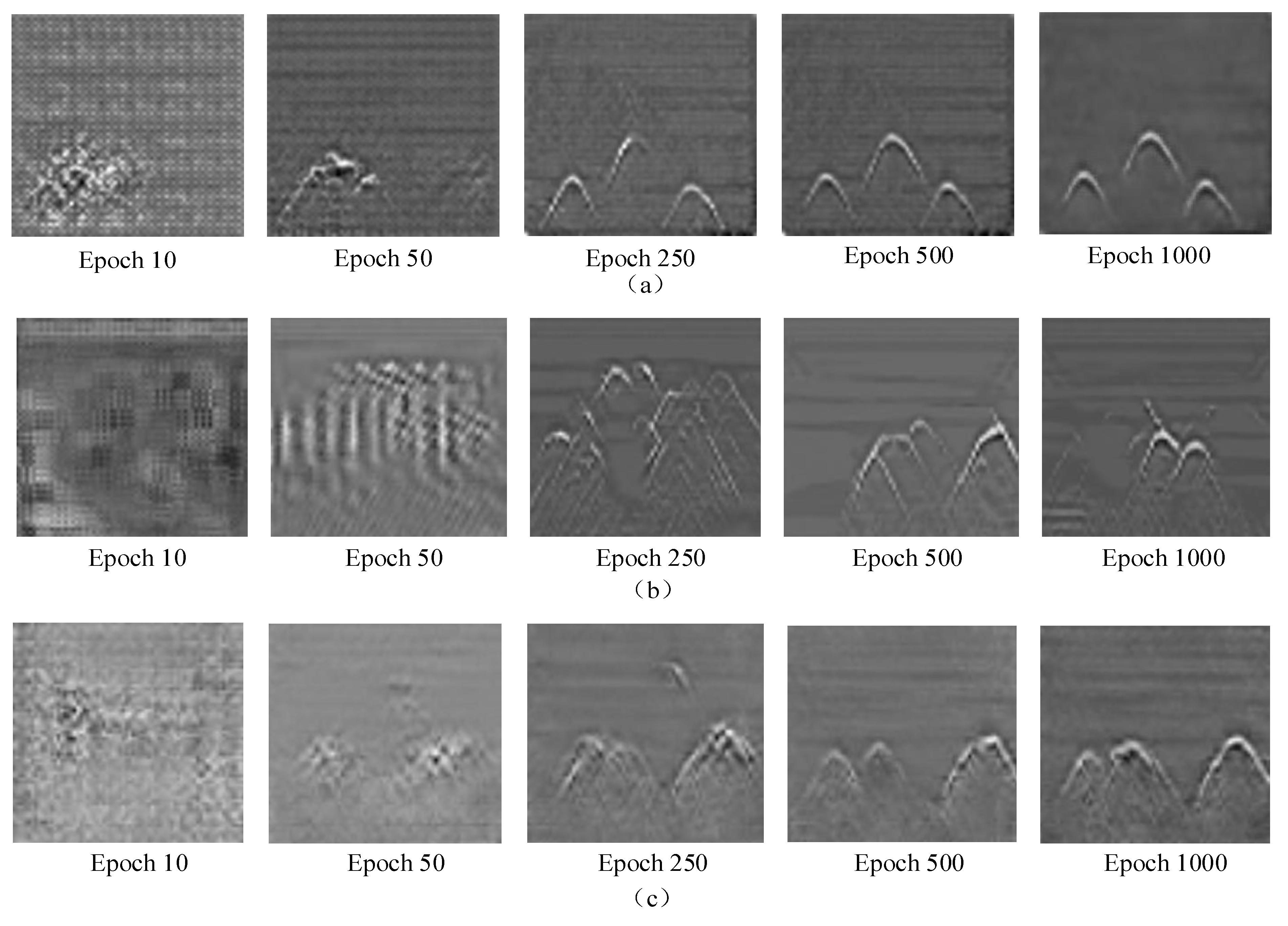
A visual inspection of the WGAN training process is displayed in Figure 4a. The generator of WGAN learnt the hyperbolic characteristics of GPR images from the training dataset and updated the network parameters under the guidance of the discriminator to generate realistic GPR images. The generated image started from an image with random noise. After 10 epochs, there was a concentration of noise in the generated image. After 50 epochs, some prominent features appeared in the generated image, but it lacked details. When it reached 250 epochs, some subtle features similar to the reflection of rebar were observed, but there were cases where the tail of the hyperbola was missing. After 500 epochs, the generated image revealed more details and was very similar to the real GPR image. Figure 4b,c shows that when the epoch was 1000, the hyperbola of GPR image generated by DCGAN and ACGAN was still blurred, while the image generated by WGAN was clear and realistic. Therefore, the performance of WGAN was better than that of DCGAN and ACGAN. With the help of well-trained WGAN, we were able to generate 3200 generated images to expand the MCAE training dataset.

4.2. Denoising Results by MCAE

After data augmentation, the dataset contained 400 field GPR images, 1400 FDTD-simulated images, and 3200 WGAN-generated images. A total of 5000 noise-free GPR images were used as the label. Then, these 5000 images were added with noise to form the noisy dataset of MCAE, for which PSNR was 11.0 dB. Among them, 4000 (80%) noisy GPR images were used as the training dataset to train the MCAE model, and the remaining 1000 (20%) were used as the test dataset to test the MCAE model performance.

In the training process of the MCAE model, for each noisy GPR image, the data format was first converted, and the size of the converted image was 256 × 256 × 1. The input noisy image was encoded and compressed into a low-dimensional feature map by the MCAE encoder, and the denoised image was output through the decoder. After that, the mean square error between the image output by the decoder and the noise-free GPR image was calculated, and the weight parameters of MCAE were continuously optimized through the reverse gradient propagation algorithm to reduce the mean square error. In the experiment, the batch size was set to 100, and the learning rate was set to 0.000005. After 400 epochs, the mean square error L stabilized, and the model was well trained. As shown in Figure 5, after implementing the data augmentation method, we found that the model converged faster, and the stable loss value was lower.

In the verification stage, the noisy image was put into the trained MCAE model, and the denoised GPR image was reconstructed and output through encoding and decoding. The peak signal-to-noise ratio (PSNR) of the denoised image was calculated. The calculation expression of PSNR is shown as follows:

$$\mathrm{PSNR}=10{\log }_{10}\frac{{(2^a-1)}^2}{\frac{1}{M\times N}{\displaystyle \sum _{m=1}^M{\displaystyle \sum _{n=1}^N{\Vert {\widehat{y}}_{m,n}-y_{m,n}\Vert }^2}}}$$

(10)

where $y_{m,n}$ represents the value of the m-th row and n-th column of the noise-free GPR image; ${\widehat{y}}_{m,n}$ represents the value of the m-th row and n-th column of the GPR image after denoising; and M and N are the height and width of the image, respectively. a is the bit per pixel and is usually set to 8, which means that the number of pixel gray levels is 256. The larger the PSNR value, the smaller the distortion.

The experimental results are shown in Figure 6. In the simulated image, the noisy GPR image with PSNR of 11.23 dB was denoised by MCAE, and its PSNR can be increased to 30.18 dB. In the field image, the noisy GPR image with PSNR of 11.25 dB was denoised by MCAE, and its PSNR can be increased to 32.41 dB. In the generated image, the noisy GPR image with PSNR of 11.28 dB was denoised by MCAE, and its PSNR can be increased to 31.82 dB.

4.3. Comparison of Experimental Results

The proposed MCAE algorithm was compared with several state-of-the-art image denoising methods, including BM3D, WNNM, NLM, and CAE. The classic Wavelet denoising method was also compared. PSNR is an important performance metric in terms of analyzing the performance of the different denoising methods; in addition, the structural similarity index (SSIM) and time cost were also introduced to analyze the different denoising methods. The value range of SSIM was between 0 and 1. The larger the SSIM value, the smaller the image distortion.

We evaluated the competing methods on 30 test images consisting of 10 simulated images obtained by the gprMax tool, 10 field images obtained by SIR 4000, and 10 generated images obtained by WGAN. Figure 7 shows the image scenes. Zero mean additive white Gaussian noise with different standard deviations (σ = 10, 30, 50, and 70) were added to these test images to generate the noisy images.

Table 1. Average PSNR (dB) for different standard deviations with various denoising methods.

-	Noisy Image	Proposed	CAE	NLM	WNNM	BM3D	Wavelet
σ = 10	Simulated images	31.61	30.46	30.77	28.89	30.95	29.92
	Field images	38.12	35.62	34.36	36.98	38.92	38.06
	Generated images	36.35	32.68	32.12	32.53	36.59	35.74
σ = 30	Simulated images	30.61	28.92	29.13	28.75	29.96	28.66
	Field images	35.82	32.56	31.50	32.63	31.85	30.23
	Generated images	34.42	32.46	30.83	30.63	31.36	29.83
σ = 50	Simulated images	30.39	27.64	16.12	27.92	25.95	25.61
	Field images	33.32	30.89	15.44	29.14	27.24	26.15
	Generated images	32.66	29.72	16.60	29.83	26.82	26.22
σ = 70	Simulated images	30.18	27.18	12.28	27.81	22.56	23.67
	Field images	32.41	30.34	15.98	27.09	24.51	23.69
	Generated images	31.82	28.23	12.43	28.67	21.85	23.74

shows the PSNR results of different denoising methods. The result for each image and on each noisy level is highlighted in bold, which denotes the highest PSNR. The proposed MCAE achieved the highest PSNR in almost every case. When the noise level was relatively low (σ = 10), on the simulated image, the proposed method achieved the highest PSNR of 31.61 dB. On the field and generated images, the BM3D method achieved the highest PSNRs of 38.92 dB and 36.59 dB, respectively. However, as the noise level continued to increase (σ = 30, 50, and 70), the performance of the proposed method could be maintained, and it achieved the highest PSNR on all images. This was followed by CAE and WNNM methods, which could also maintain a relatively high PSNR. However, when the noise level σ exceeded 50, the PSNR values achieved by both BM3D and Wavelet were relatively low, and the NLM method was not even effective. These indicate that the proposed MCAE method is more robust to noise intensity than other methods.

Table 2. Average SSIM for different standard deviations with various denoising methods.

-	Noisy Image	Proposed	CAE	NLM	WNNM	BM3D	Wavelet
σ = 10	Simulated images	0.91	0.86	0.85	0.89	0.91	0.87
	Field images	0.95	0.93	0.93	0.95	0.95	0.93
	Generated images	0.93	0.88	0.87	0.90	0.92	0.90
σ = 30	Simulated images	0.87	0.85	0.78	0.84	0.71	0.68
	Field images	0.94	0.92	0.84	0.93	0.76	0.74
	Generated images	0.90	0.87	0.80	0.86	0.72	0.69
σ = 50	Simulated images	0.89	0.82	0.20	0.81	0.47	0.51
	Field images	0.93	0.90	0.21	0.90	0.57	0.56
	Generated images	0.86	0.83	0.19	0.84	0.46	0.52
σ = 70	Simulated images	0.85	0.79	0.11	0.82	0.42	0.43
	Field images	0.92	0.89	0.12	0.88	0.52	0.44
	Generated images	0.85	0.81	0.09	0.83	0.37	0.41

shows the SSIM results of different denoising algorithms. In each noise level, the highest SSIM result of each image is bolded. In all four noise levels, the proposed method achieved the highest SSIM. Under a low noise level (σ = 10), BM3D and WNNM achieved the same SSIM of 0.95 as the proposed method on the field image, which had good denoising performance. However, as the noise level increased, the SSIM of the BM3D, Wavelet, and NLM methods dropped sharply, being lower than 0.5 when the σ was 70. The CAE method and the WNNM method can also maintain a high SSIM, but they were still lower than the proposed method.

Table 3. Average time cost (s) for different denoising methods.

Noisy Image	Proposed	CAE	NLM	WNNM	BM3D	Wavelet
Simulated images	0.242	0.227	3.865	40.56	120.71	0.751
Field images	0.240	0.231	4.062	39.67	114.37	0.762
Generated images	0.241	0.236	3.735	40.72	113.75	0.663
AVE.	0.241	0.231	3.887	40.31	116.28	0.725

shows the time cost of different denoising algorithms for processing each image. It can be seen that BM3D consumed the most time, with an average time consumption of 116.28 s on the three images, followed by WNNM, with an average time consumption of 40.31 s. Both the proposed method and the CAE method had good performance. Their average consumption times were only 0.241 s and 0.231 s, respectively, which could realize real-time processing.

In Figure 8 and Figure 9, we show a comparison of the visual quality of denoised images processed by different methods. Figure 8 shows that when the noise level was relatively low (σ = 30), all denoising methods obtained good image visual quality and the proposed method was able to reconstruct more image details from noisy observations. Figure 9 shows that when the image was at a strong noise level (σ = 70), the proposed method could still reconstruct the details of the image and maintain a clear edge structure. However, the image visual quality of other methods was greatly reduced. Compared with the MCAE method, the method such as NLM, BM3D, and Wavelet still retained a large amount of noise. Although CAE and WNNM could suppress random noise effectively, the reconstructed image lost the hyperbolic tail features and edge information. In summary, MCAE had a powerful denoising ability, producing a visually pleasing denoising output while having higher PSNR.

5. Conclusions

In this paper, we propose a scheme for GPR image denoising based on DL techniques, which consisted of WGAN and MACE. The MCAE algorithm improved the CAE model by introducing a multi-scale convolution kernel to extract higher-level features of the image. The WGAN was designed for increasing the GPR images to solve the problem of insufficient MCAE training dataset. The MCAE achieved a better denoising effect with the data augmentation. The experimental results showed that MCAE could not only bring significant PSNR improvements over state-of-the-art methods such as CAE, WNNM, and BM3D, but also could reconstruct better local structures of the image and less visual artifacts. However, the factors that affect GPR image quality included not only random noise but also clutter caused by multi-target interference. In future work, we will continue to study the methods based on DL technology to remove the GPR image clutter.