Mitigation of the Effects of Network Outage on Video QoE Using a Sender Buffer

Abstract

With the growth of multimedia applications and the mobile Internet, quality sense and quality expectation of the end-user are rising rapidly. A small notable distortion in the multimedia applications may degrade the degree of delight of the user, who is very considerate of the video Quality of Experience (QoE). During live streaming, a network outage may result in video freezes and video jumps. To dampen the impact of a network outage on the video QoE, we propose the use of a well-sized sender buffer. We present the concept, derive key analytical relations, and perform a set of subjective tests. Based on those, we report a significant enhancement of user ratings due to the proposed sender buffer in the presence of network outages.

1. Introduction

The use of multimedia applications is tremendously increasing with the rapid growth of wireless and mobile wireless Internet. Mobile devices, such as smartphones, pads, and laptops, are capable of connecting to the Internet via mobile (e.g., 3G, 4G, or 5G) and wireless (Wi-Fi) interfaces. Moreover, mobile devices are continuously improving in terms of computing capabilities and power, data speed, and screen resolution. This exposure strengthens the quality sense of the user, and she expects a good Quality of Experience (QoE), describing the degree of delight or annoyance of a user’s experience with a service [1]. However, multimedia applications are sensitive to jitter, bandwidth limitation, and delay. The disruption of the network is more noticeable in multimedia applications than in other applications. As glitches and artifacts are more perceivable in multimedia applications, they can easily affect users’ QoE. Live video transmission may undergo QoE degradation due to interruptions such as video freezes, jumps, and misses.

The use of Internet services increased by factor 2.5 as compared to COVID-19 pre-lockdown [2]. Due to the COVID-19 pandemic, many businesses and other activities have moved online. This increases the use of live multimedia applications, e.g., online meetings, lectures, discussions, etc. For example, during an online lecture, when a teacher is teaching, the students may miss key information and lecture material due to a network problem. Similarly, watching a cricket match online and missing a big shot of six of one’s favorite team can dramatically lower QoE ratings. We will see subsequently that buffering some content on the sender-side can help with mitigating the impact of network problems on QoE and its ratings, especially when buffered data are sent to the recipient at a higher rate than the required data rate. The theoretical download speed of 5G ranges from 1 Gbps to 10 Gbps, and the average download speed of 5G is 50 Mbps and above [3]. Therefore, getting high data rates in 5G is not a big challenge.

Nowadays, the user has more options to select both network provider and service provider. One may leave or join a network or a service provider based on personal or cumulative QoE ratings. Thus, in this user-centric era, the satisfaction and good perception of users are vital for the network providers and service providers to survive in the competitive market. Studying QoE and related user perception has been attracting the attention of researchers, manufacturers, network, and service providers for about two decades. In Reference [4], the authors discuss the QoE management challenge for multimedia applications and also identify future research directions. In References [5,6,7,8], the authors have studied video QoE related to network performance parameters, while others also have looked into web QoE [9,10]. In these studies, the parameters of interest are network performance parameters and their impact on QoE. Despite the advances of networks and mobile devices, maintaining acceptable QoE under the Internet’s best-effort networking paradigm is a challenge. The transmitted data suffer from impairments through both transmissions over congested links and error-prone channels. This results in a degradation of user ratings. The most frequent network-induced issues that arise with video transmission are throughput variability, packet loss, packet delay, and packet delay variation. The receiver buffer is used to accommodate throughput variability and jitter. It stores the data temporarily to smooth the throughput variation and the jitter, and provides data with the required data rate to the client. The receiver buffer is also referred to as the jitter buffer in this article.

The packet delay variation in the Internet is very small, and is typically measured in milliseconds. However, in the case of mobile Internet, it may reach the order of seconds, which is jitter of a completely different order of magnitude that has to be taken care of by a properly dimensioned jitter buffer. In Reference [11], the authors measured the one-way delay on the down-link in mobile networks and realised spans of one-way delays (OWD) between less than 50 ms to 2.1 s and beyond. Similar results were reported in [12], in which the authors performed active delay measurements in the 3G HSPA network on the application level. Long delays in the down-link at the application layer in the live stream may empty the jitter buffer. This results in video freezes, which may hamper the user’s QoE. Moreover, it may happen that the receiver is not receiving any valid data during periods due to other reasons such as bit errors corrections, handoffs, congestion, etc. In Reference [13], the authors built an argument based upon previous studies that handover delay and packet loss due to path change and binding updates may degrade the QoS. In Reference [14], the authors reported that, from server to UE, some pings experienced long RTTs (>500 ms) as compared to the expected RTTs of 35 ms with a 100% success rate on handover. The consequence of such communication break is a paused play-out until new data are available. During the live streaming, when the sender is sending continuously, data may be lost during such a network outage. In this case with paused play-out, the user may miss multimedia content. This phenomenon is more likely to appear in mobile and wireless networks as compared to wired networks. In the case of video streaming, video freezes degrade the QoE of the user remarkably [15,16]. Multiple freeze events have a severe impact on QoE, while the impact of data loss also depends on the video content [17].

Along with the evaluation of QoE, various efforts have been made to maintain an acceptable level of QoE. These efforts included the use of different codecs, error recovery schemes, recovery of the lost or dropped frames, jitter buffer, lost packet recovery, and so on. A dynamic transport architecture was proposed for next-generation mobile networks adapted to video service requirements and aiming at improving the QoE [18]. In Reference [19], the authors proposed an intelligent packet drop concept to improve the QoE in case of congestion.

In this article, we propose a solution by using a sender buffer for the live video stream to diminish the impact of the network outages, which may be the result of the delay, hand-off, or any other network interruption, on video QoE. The proposed approach can be implemented within the existing setup and within the available resources.

The first part of the article covers the theoretical modeling, analysis, discussion, and comparison of the proposed solution with existing streaming service configuration. We also discuss the proper dimensioning of the sender buffer size in relation to the jitter buffer.

The second part of the article discusses the experimental result of videos streamed without and with the proposed sender buffer solution, in the presence of network outages. The experimental data are statistically analyzed, in terms of Mean Opinion Scores (MOS) and MOS gains due to sender buffer as well as due to increased transmission rates between sender and receiver buffer.

Moreover, to the best of our knowledge, there is no specific work in which the sender buffer is used only on a need-basis to resolve the network outage problem, nor has there been any study that is addressing the dimensioning of the sender buffer in comparison to the jitter buffer for optimizing QoE, which are the main contributions of this article.

The remainder of the paper is organized as follows: Section 2 presents related work. Section 3 describes artifacts in video delivery and play-out, such as freezes, jumps, and misses. Section 4 elaborates on the video stream, while Section 5 discusses the proposed video stream model. Section 6 explains the role of the jitter buffer in multimedia streaming, and Section 7 figures out the role of the sender buffer in relation to the receiver buffer. Section 8 covers the discussion of the analytical part. Section 9 provides the user ratings of videos for different scenarios and compares the existing and proposed streaming approaches in terms of the user ratings. Finally, Section 10 concludes this article.

2. Related Work

The data packets that constitute a live stream over a network may experience varying OWD, which is usually referred to as packet delay variation or jitter [20]. There are many reasons for such kind of behavior: Different queues (at sender, receiver and in the network), network congestion, route changes, or mobile or wireless link layer impairments are major causes for varying OWD of packets. For instance, the error correction of the radio channels usually delivers error-free packets using the Automatic Repeat reQuest (ARQ) process at the price of jitter [21].

In multimedia applications, a stream whose packets are affected by jitter may create artifacts and degrade user perception, due to late arrival of essential information. In Reference [22], the authors used the measured Quality of Service (QoS) distribution to evaluate the distribution of QoE metrics. In Reference [23], the authors investigated the buffer size and video QoE for Netflix and found that improved buffer size can improve the video QoE. In addition, they found that TCP Reno with a smaller buffer is causing higher loss and has a negative impact on applications. In Reference [24], the authors examined latency and throughput in the face of heterogeneous buffer sizes of the network router for live video streaming application, and recommended the middle-of-the-road scope of buffer sizes. As many others, these rather recent publications focus on TCP-based content streaming, as opposed to UDP-based live streaming as addressed by our work.

In Reference [25], the authors studied the effect of jitter on the perceptual video quality and found that even low amounts of jitter or packet loss degrade the video quality severely as compared to the perceptual video quality of the reference video. To overcome the after effects of the jitter, and to smooth the incoming stream, jitter buffer is used. The jitter buffer plays a useful role in multimedia streaming by buffering the variable-rate data and maintains the required data rate for playback. However, the jitter buffer compensates the jitter at the expense of latency. Different efforts have been made to manage the jitter for multimedia applications [26,27]. In Reference [28], the authors proposed a mechanism by distributing the buffer space requirements more uniformly over the route of an end-to-end path to control the jitter for packet-switching internetworks.

The size of the jitter buffer can vary according to the requirement of the application and the availability of resources. The data in the jitter buffer may shrink or expand. The size of the jitter buffer is a trade-off between the initial play-out delay and packet loss. To reduce the initial delay, a jitter threshold level is set for data in the jitter buffer, from where play-out begins. The jitter threshold level is smaller than the jitter buffer. The threshold level of the jitter buffer is very critical because the initial delay of the video depends on the threshold level. The threshold level of the jitter buffer should not be so small that the player consumes the buffer data during a very short period of time, which may anyway result in a video freeze. Moreover, a comparably high threshold level of jitter buffer may increase the initial delay which may degrade the user experience [29]. Similarly, after a network outage, it may take longer to restart playout, also resulting in a poor user experience.

To maintain the QoE and for smooth play-out of multimedia content on the Internet various efforts have been made besides the use of a jitter buffer. The use of the sender buffer is one of them. In Reference [30], the authors propose a buffer-driven adaptation streaming scheme for a stored video, which scales the quality of transmission, based on both receiver buffer occupancy and sender buffer occupancy, instead of bandwidth. In Reference [31], the authors investigate the double-buffer traffic shaper, implemented using Token and Leaky Bucket techniques, to adjust the video frame rate inflow into the TCP sender buffer of a multimedia application source across a slow-speed link. The authors of [32] introduced a scheduling algorithm based on the sender buffer backlog for real-time application. It schedules time slots based on the sender buffer backlog at the base station, which is believed to be correlated with a play-out buffer backlog at the receiver.

In Reference [33], the authors proposed enhanced transport named paceline to improve the performance and availability of streaming video and time-sensitive media by reducing the TCP queuing delay at the sender-side. To address the shortcoming of the existing error control solution for real-time streaming, the authors of [34] proposed packet reliability-based real-time streaming (RERES). In this solution, the authors came up with scheduling algorithms for reliable adaptation and buffer control. In Reference [35], the authors proposed to send all the packets via sender buffer using a UDP socket. On receiving negative acknowledgment packets (NAK), based on previous information and the sender buffer level, they decide whether to retransmit the video packet or not. The important factors used for the decision of retransmission of a video packet are the timeout counter and transmission rate.

3. Video Freeze, Jump, and Miss Artifacts

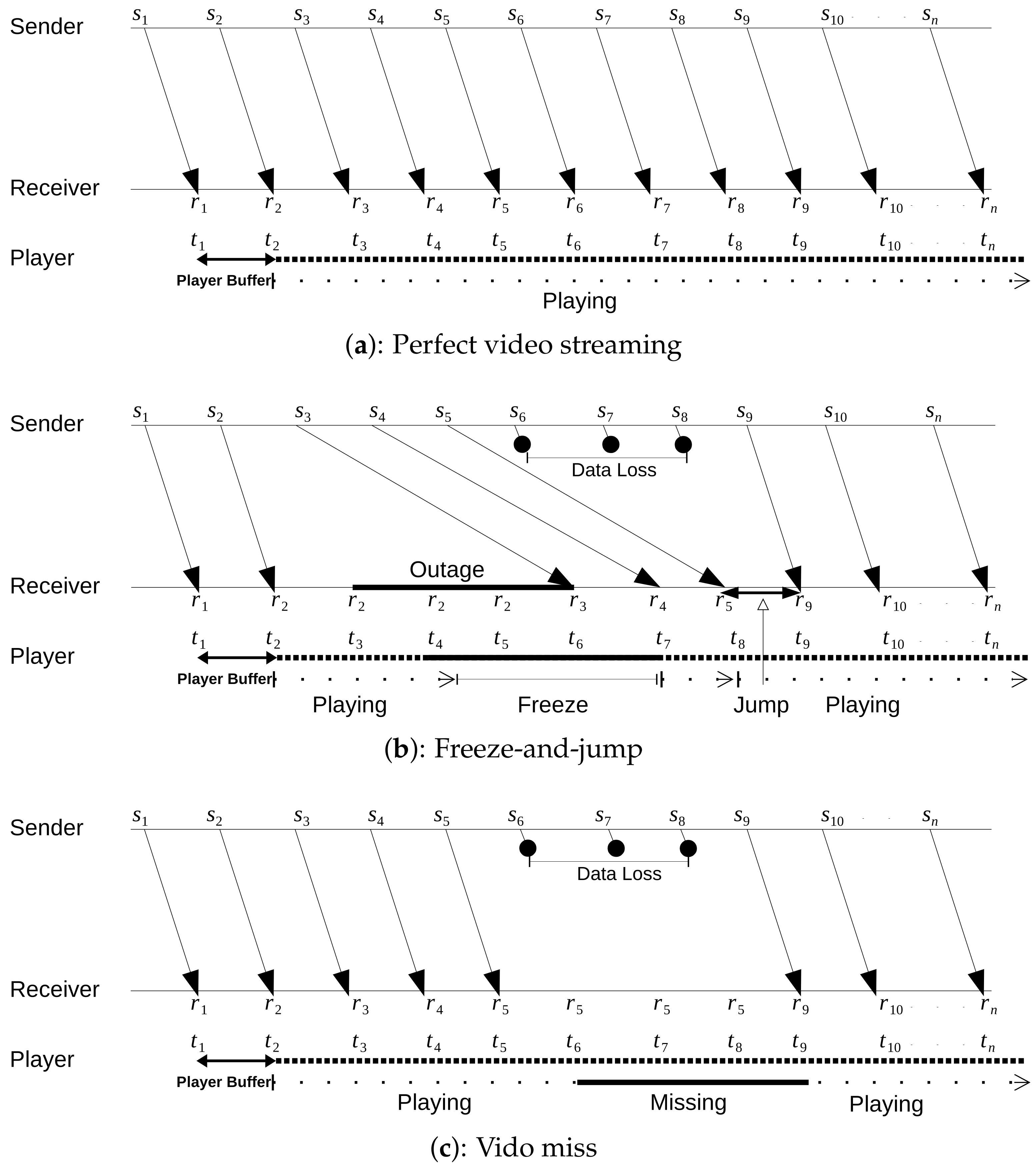
During live video transmission over an error-prone channel, data may be lost or delayed. As a result, the user may face temporal artifacts. Along with other temporal artifacts, video freezes, jumps, and misses are the common artifacts of live video transmission. Figure 1 illustrates the freeze, jump, and miss artifacts of video streaming.

Perfect Video Streaming: Figure 1a shows video streaming without any artifact like freeze-jump and miss. Initially, the player fills the player buffer before starting the play-out. After that, if the arrival rate of data is not less than the playing rate, the video will play smoothly.

Video Freeze-and-Jump: Video freeze-and-jump occurs due to excessive delay or data loss. On regaining the network, the on-demand video starts playing from the frame where it stalled. However, in the case of live transmission, video starts playing from the new frame that is transmitted at that instant. Figure 1b demonstrates the freeze-and-jump case. After receiving the video chunk ${\mathrm{r}}_2$ at time $t_2$, the video stream stopped due to network outage and resumed back at time $t_6$. The player remains halted at the last displayed picture ${\mathrm{r}}_2$ for the duration of $t_2$ to $t_6$. The freeze-time is the time duration for which the player remains paused at the last displayed frame, without losing the connection with the server.

In video streaming, there are several causes of data loss, such as intermediate buffer overflow, network outage, etc. As a result of this data loss, the player jumps from the last successfully played frame to the new correctly received frame. Figure 1b explains the jump of the video, after playing ${\mathrm{r}}_5$, the player jumps to ${\mathrm{r}}_9$ in the next time interval. The video jump-length is the duration of the skipped video due to data loss, which is a result of a network outage.

Video Miss: In live streaming, usually, the video freeze is followed by a video jump. However, when freeze-and-jump both take place together simultaneously, this implies a video miss, depicted in Figure 1c. The miss-time is the time interval for which video freeze and jump occur simultaneously.

4. Live Video Streaming

Video streaming requires a steady frame rate for smooth play-out. However, during the transmission of the data over the networks, packet arrival time may vary due to congestion, time drift, routing, etc. This irregularity in the arrival time of the packets is called jitter. To combat the jitter, a jitter buffer or receiving buffer is used at the receiving end. The presence of a jitter or application buffer is very common in multimedia applications [36]. However, the jitter buffer introduces some initial delay equal to the time length of the jitter in the play-out. Larger jitter buffers provide more tolerance to the streaming applications, as they have enough data to support the play-out during the network disturbance. Nevertheless, a larger jitter buffer increases the initial delay, and the user needs to wait extra time during re-filling of the larger buffer.

A jitter buffer is measured in time units (typically milliseconds) and can be sized to the number of video frames. Let ${\tau }_{\mathrm{j}}$ represent the jitter buffer in time units. In the presence of ${\tau }_{\mathrm{j}}$, the end-user will face an initial delay $d_{\mathrm{i}}$ equal to ${\tau }_{\mathrm{j}}$, when starting the video play-out. The jitter buffer usually has a minimum threshold level, from which the play-out begins. However, for the sake of simplicity of the discussion, the size of jitter buffer is considered equal to the player buffer threshold to start the playing.

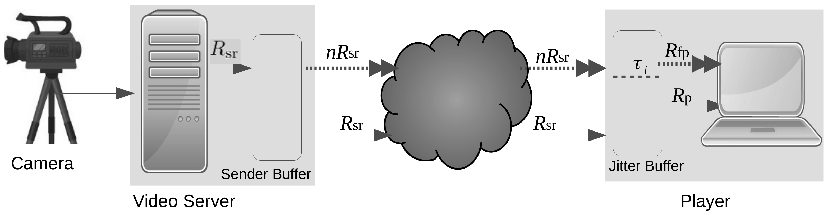
Figure 2 shows the video streaming model, which includes the camera attached to the sender and the jitter buffer players. Let us assume that the receiver is receiving the video from the sender with the data rate $R_{\mathrm{sr}}$, and the jitter buffer can be filled with this data rate in time ${\tau }_{\mathrm{j}}$. Then, the size of jitter buffer is given as

$$X_{\mathrm{sr}}^{{\tau }_{\mathrm{j}}}=R_{\mathrm{sr}}{\tau }_{\mathrm{j}}$$

(1)

The player starts consuming the data from the jitter buffer after the initial delay $d_{\mathrm{i}}$. The initial delay is the time needed to fill the jitter buffer up to threshold level ${\tau }_{\mathrm{j}}$. Once the jitter buffer is full and ready, the player starts consuming the data. Let $R_{\mathrm{p}}$ be the video consumption rate, i.e., the decoding rate for smooth play-out. For smooth play-out, $R_{\mathrm{sr}}$ should not be smaller than $R_{\mathrm{p}}$; otherwise, the jitter buffer may underrun. Consequently, the video will freeze until re-buffering is over. In this case, play-out and freeze occur periodically.

Moreover, the jitter buffer may underrun due to network outage. The latter is a temporary downtime of network, during which the data flow is interrupted. It may occur due to network performance issues, such as loss of link, delay, handover, packet loss, etc. The outage duration ${\tau }_{\mathrm{o}}$ refers a time-period in which the network fails to deliver valid data to the receiver.

Due to a network outage and a subsequent underrun of the jitter buffer, the video will freeze at play-out. When a channel becomes available again after a network outage, the restart of the play-out depends on a number of factors, such as packet loss, loss recovery, and loss flexibility of the codec. The authors of [7] have discussed these factors as Quality of Delivery (QoD) and how the QoD has an impact on the QoE. The play-out may restart from the freeze frame or jump to the new location of video by skipping the video equal to the duration of the outage. If the retransmission is possible, then the video play-out restarts from the freezing point. Otherwise, play-out restarts from the newly arrived frame, i.e., there is no retransmission. For example, in live transmission, after the network outage, there is no option to retransmit the data transmitted during the network outage unless it was saved for retransmission at the sender. In case of live transmission, network outage may entail video freeze-and-jump. In this case, the video freeze duration $F_{\Delta t}$ and amount of data lossL are directly proportional to the outage duration.

The video freeze-and-jump has an adverse impact on the user QoE [15,16,29]. In case of a video jump, users may feel to be deprived for missing video content of an important moment, e.g., a goal or an attempt for goal in a soccer match, and this may degrade the user QoE. The length of freeze-and-jump depends on the duration of outage. To reduce the duration of these artifacts and to improve the QoE of the user, we propose a buffer at the sender side to save the data during the network outage.

Before discussing the proposed model, we present the variables and related key relations used in this article in

Table 1. Terminology used.

Variable	Description	Expression
C	Capacity of the channel between sender and receiver	$C=n{R}_{\mathrm{sr}}$ for $n>1$
$F_{\Delta t}$	Video freeze duration due to outage
L	Data loss during the outage
n	Capacity factor
$R_{\mathrm{sr}}$	Data rate from sender to receiver for smooth play-out
$R_{\mathrm{p}}$	Player data consumption rate for smooth play-out
$t_{\mathrm{e}}\left({\tau }_{\mathrm{s}}\right)$	Time to empty the sender buffer at data rate C	$t_{\mathrm{e}}\left({\tau }_{\mathrm{s}}\right)=\frac{{\tau }_{\mathrm{s}}}{n-1}$ for $n>1$
$t_{\mathrm{f}}\left({\tau }_{\mathrm{j}}\right)$	Time to fill the jitter buffer at data rate $n{R}_{\mathrm{sr}}$	$t_{\mathrm{f}}\left({\tau }_{\mathrm{j}}\right)=\frac{{\tau }_{\mathrm{j}}}{n}$
${\tau }_{\mathrm{o}}$	Network outage duration
${\tau }_{\mathrm{j}}$	Time to fill the jitter buffer at data rate $R_{\mathrm{sr}}$
${\tau }_{\mathrm{s}}$	Time to fill the sender buffer at data rate $R_{\mathrm{sr}}$
$X_{\mathrm{s}r}\left({\tau }_{\mathrm{j}}\right)$	Data buffering capacity of the jitter buffer at data rate $R_{\mathrm{sr}}$	$X_{\mathrm{s}r}\left({\tau }_{\mathrm{j}}\right)=R_{\mathrm{sr}}{\tau }_{\mathrm{j}}$
$X_{\mathrm{s}r}\left({\tau }_{\mathrm{s}}\right)$	Data buffering capacity of the sender buffer at data rate $R_{\mathrm{sr}}$	$X_{\mathrm{s}r}\left({\tau }_{\mathrm{s}}\right)=R_{\mathrm{sr}}{\tau }_{\mathrm{s}}$
$X_{{\tau }_{\mathrm{s}}}\left({\tau }_{\mathrm{o}}\right)$	Data sent to the sender buffer during the network outage	$X_{{\tau }_{\mathrm{s}}}\left({\tau }_{\mathrm{o}}\right)=R_{\mathrm{sr}}{\tau }_{\mathrm{o}}$

.

5. Proposed Video Streaming Model

Figure 3 illustrates the proposed video streaming model, which consists of a receiver and a proposed sender buffer. The sender sends the data directly to the receiver while the sender buffer is used under adverse conditions. In case of network outage, the sender’s data are stored in the sender buffer. After the outage, when the channel gets available again, the sender buffer provides the saved data for quick rebuffering of the jitter buffer, which may be empty due to the outage. For quick rebuffering of the jitter buffer, it is assumed that the sender transmits the buffered data with maximum possible capacity

$$C=n{R}_{\mathrm{sr}}\mathrm{where}n>1$$

(2)

If the sender fails to send the buffer data with higher speed, i.e., if $n=1$, then the sender buffer may not be emptied at the end of the transmission. In this case, it is up to the user to play delayed video or skip the sender buffer content to watch the video in real time. Thus, a higher data speed $(n>1)$ is required to empty the sender buffer and get back the video in real time.

The presence of the sender buffer helps to save the data during the outage and reduces the video freeze time, which is described through the following key formulae for data loss (3) and freeze time (4)

$$L=R_{\mathrm{sr}}({\tau }_{\mathrm{o}}-min\{{\tau }_{\mathrm{s}},{\tau }_{\mathrm{j}}\})\mathrm{where}{\tau }_{\mathrm{o}}\ge min\{{\tau }_{\mathrm{s}},{\tau }_{\mathrm{j}}\}$$

(3)

$$F_{\Delta t}={\tau }_{\mathrm{o}}-min\{{\tau }_{\mathrm{s}},{\tau }_{\mathrm{j}}\}\left(1-\frac{1}{n}\right)\mathrm{where}{\tau }_{\mathrm{o}}\ge min\{{\tau }_{\mathrm{s}},{\tau }_{\mathrm{j}}\}$$

(4)

The derivation and discussion of Equations (3) and (4) will follow in Section 7 and Section 8, respectively.

There will be no data loss if the outage duration ${\tau }_{\mathrm{o}}$ is smaller than or equal to ${\tau }_{\mathrm{s}}$. However, if ${\tau }_{\mathrm{o}}$ is greater than ${\tau }_{\mathrm{s}}$, then data will be lost due to overflow of the sender buffer. Moreover, any network outage ${\tau }_{\mathrm{o}}$ greater than the jitter buffer ${\tau }_{\mathrm{j}}$ results in a video freeze equal to ${\tau }_{\mathrm{o}}$. The minimum duration of the video freeze the user has to face is the time to re-fill the empty jitter buffer to start the play-out. After the outage, this freeze duration can be reduced by flushing the sender buffer data with maximum channel capacity C. In this way, the sender buffer is used for saving the data during the outage and reducing the freeze duration after the outage.

In the following sections, we will quantify and discuss the usefulness of sender buffer, along with the jitter buffer, in detail. In Section 6, we will discuss the role of the jitter buffer in multimedia streaming without sender buffer using Equations (3) and (4). In addition, Section 7 and Section 8 will estimate the size of the sender buffer corresponding to the size of the jitter buffer.

6. The Role of the Jitter Buffer in Live Multimedia Streaming

To overcome the after effects of the jitter, and to smooth the incoming stream, an application jitter buffer is used. The size of the jitter buffer can vary according to the requirement of the application and the availability of resources. The data in the jitter buffer may shrink or expand. As mentioned earlier in this article, the size of the jitter buffer is considered equal to the threshold of the jitter buffer from where the play-out starts.

In case there was only the jitter buffer, then ${\tau }_{\mathrm{s}}=0$. If ${\tau }_{\mathrm{o}}<{\tau }_{\mathrm{j}}$, then, during the network outage, the jitter buffer will not become empty, and the user will not see any impact on play-out. On the other hand, if ${\tau }_{\mathrm{o}}\ge {\tau }_{\mathrm{j}}$, then, during the network outage, the jitter buffer will dry-out, and the user will face data loss and video freeze.

With ${\tau }_{\mathrm{s}}=0$ in (3), we obtain

$$L=R_{\mathrm{sr}}({\tau }_{\mathrm{o}}-min\{0,{\tau }_{\mathrm{j}}\})=R_{\mathrm{sr}}{\tau }_{\mathrm{o}}\mathrm{for}{\tau }_{\mathrm{o}}\ge {\tau }_{\mathrm{j}},\mathrm{i}.\mathrm{e}.,L\propto {\tau }_{\mathrm{o}}$$

(5)

The data loss is proportional to the network outage. Thus, all data sent during the network outage will be lost.

Similarly, by using Equation (4), the video freeze duration can be calculated as

$$F_{\Delta t}={\tau }_{\mathrm{o}}-min\{0,{\tau }_{\mathrm{j}}\}\left(1-\frac{1}{n}\right)={\tau }_{\mathrm{o}}\mathrm{for}{\tau }_{\mathrm{o}}\ge {\tau }_{\mathrm{j}},\mathrm{i}.\mathrm{e}.,F_{\Delta t}\propto {\tau }_{\mathrm{o}}$$

(6)

which shows that the video freeze duration will be equal to that of the network outage.

In the absence of the sender buffer, the network outage results in the jump-and-freeze artifact, the length of which is determined by the duration of the network outage.

7. The Role of the Proposed Sender Buffer in Live Multimedia Streaming

The proposed sender buffer at the sender provides the option to save the data during the network outage. During a normal flow of data, the sender sends the data directly to the receiver. However, during a network outage, the sender saves the data in sender buffer. After the network outage, the sender sends that data through the sender buffer unless the sender buffer empties. As a result, the user receives delayed data until the sender buffer is empty. It is important to empty the sender buffer as quickly as possible to get the live stream back.

To recover the live stream in a shorter time, it is necessary to flush the sender buffer data with maximum channel capacity. In this way, the sender buffer helps to save the data and reduce the video freeze duration by quickly re-filling the jitter buffer. Ultimately, it improves the user video QoE. Thus, the outlet data rate must be greater than the inlet data rate of the sender buffer. Otherwise, if the inlet and outlet data rates of the sender buffer are the same, then the user may not get the live data stream back. If the sender buffer holds data, then the sender sends data through the sender buffer. As a result, the sender buffer will not empty, and the user will face latency equal to the sender buffer time, i.e., ${\tau }_{\mathrm{s}}$.

If a higher data rate is not achievable, then the user may have to skip the sender buffer data to get the live stream. Hence, a higher bit rate for the sender buffer data is an important and required factor in this proposed solution. Otherwise, no timely recovery is possible.

In live transmission, the sender continuously transmits data regardless of the network status. The sender buffer saves the data during the network outage and reduces the freeze time after the network outage. During the network outage, the player continues the play-out unless the jitter buffer dries out. The corresponding video freeze starts at this moment and ends when the jitter buffer gets re-filled. The video freezes duration ($F_{\Delta t}$) depends on the network outage duration (${\tau }_{\mathrm{o}}$), time length of jitter buffer (${\tau }_{\mathrm{j}}$), and time to re-buffer the jitter buffer $t_{\mathrm{f}}\left({\tau }_{\mathrm{j}}\right)$:

$$F_{\Delta t}={\tau }_{\mathrm{o}}-{\tau }_{\mathrm{j}}+t_{\mathrm{f}}\left({\tau }_{\mathrm{j}}\right)$$

(7)

During the network outage, data may be lost at the sender side when the network outage duration is bigger than ${\tau }_{\mathrm{s}}$. Similarly, after the network outage, data may be lost at the receiver side, especially when ${\tau }_{\mathrm{j}}<{\tau }_{\mathrm{s}}$ and data are sent with high speed $C>R_{\mathrm{p}}$, i.e., the player consumption rate. The total data loss (L) is the sum of data loss at the sender ($L_{\mathrm{s}}$) and the data loss at the receiver ($L_{\mathrm{r}}$), given by

$$L=L_{\mathrm{s}}+L_{\mathrm{r}}$$

(8)

After the network outage, the amount of time it takes until the play-out restarts depends on the time to fill up the jitter buffer

$$t_{\mathrm{f}}\left({\tau }_{\mathrm{j}}\right)=\frac{{\tau }_{\mathrm{j}}}{n}$$

(9)

Similarly, after the network outage, it is also important how fast the user gets to see the live stream. Obviously, this depends on the time it takes to empty the sender buffer

$$t_{\mathrm{e}}\left({\tau }_{\mathrm{s}}\right)=\frac{{\tau }_{\mathrm{s}}}{n-1}$$

(10)

Let $\Delta t$ denote the time to get back the live stream after the play-out restarts. In the absence of the sender buffer, the time to start the smooth play-out is equal to ${\tau }_{\mathrm{j}}$. Thus, in this case,

$$\Delta t={\tau }_{\mathrm{j}}\mathrm{when}{\tau }_{\mathrm{s}}=0$$

(11)

However, in the presence of the sender buffer, $\Delta t$ depends on the time to empty the sender buffer ($t_{\mathrm{e}}\left({\tau }_{\mathrm{s}}\right)$) and the time to re-fill the jitter buffer ($t_{\mathrm{f}}\left({\tau }_{\mathrm{j}}\right)$):

$$\Delta t=\left|t_{\mathrm{e}}\left({\tau }_{\mathrm{s}}\right)-t_{\mathrm{f}}\left({\tau }_{\mathrm{j}}\right)\right|$$

(12)

The performance of the proposed sender buffer in the streaming setup can be evaluated in terms of the freeze-time ($F_{\Delta t}$), total data loss (L), and the time to get back the live stream ($\Delta t$).

As discussed, the network outage has a direct impact on the video jump and the video freeze. The presence of the sender buffer helps in reducing the length of the video jump and the video freeze. The duration of the network outage ${\tau }_{\mathrm{o}}$ may vary with respect to the size of the sender buffer ${\tau }_{\mathrm{s}}$ and the jitter buffer ${\tau }_{\mathrm{j}}$. However, the end-user will face the artifacts in the video only when ${\tau }_{\mathrm{o}}$ is greater than or equal to ${\tau }_j$. Along with the channel capacity, the performance of the proposed setup depends on the right combination of the sender buffer and the jitter buffer. With the assumption that ${\tau }_{\mathrm{o}}\ge {\tau }_{\mathrm{j}}$, the following three possible combinations are of interest:

• The sender buffer is larger than the jitter buffer;
• The jitter buffer is larger than the sender buffer;
• Sender and jitter buffer are equally sized.

7.1. Sender Buffer Is Larger Than Jitter Buffer

With given ${\tau }_{\mathrm{s}}>{\tau }_{\mathrm{j}}$, there are two possibilities with respect to the network outage. Either, the network outage is greater than or equal to the sender buffer, i.e.,

$${\tau }_{\mathrm{o}}\ge {\tau }_{\mathrm{s}}>{\tau }_{\mathrm{j}}$$

(13)

or the network outage is smaller than the sender buffer but greater than the jitter buffer, i.e.,

$${\tau }_{\mathrm{s}}\ge {\tau }_{\mathrm{o}}>{\tau }_{\mathrm{j}}$$

(14)

Let us evaluate the performance of these cases in terms of video freeze duration, data loss, and time to get back the live stream.

Video Freeze Duration (${\mathit{F}}_{\Delta \mathbf{t}}$): In both cases, either ${\tau }_{\mathrm{o}}\ge {\tau }_{\mathrm{s}}$ or ${\tau }_{\mathrm{o}}<{\tau }_{\mathrm{s}}$, the $F_{\Delta t}$ depends on ${\tau }_{\mathrm{o}}$, ${\tau }_{\mathrm{j}}$, and $t_{\mathrm{f}}\left({\tau }_{\mathrm{j}}\right)$ as given in Equation (7). The data capacity of the jitter buffer is given as

$$X_{\mathrm{sr}}\left({\tau }_{\mathrm{j}}\right)=R_{\mathrm{sr}}{\tau }_{\mathrm{j}}$$

(15)

After the network outage, the jitter buffer fills with data rate C. Thus, $t_{\mathrm{f}}\left({\tau }_{\mathrm{j}}\right)$ is given as

$$\begin{array}{c}\hfill t_{\mathrm{f}}\left({\tau }_{\mathrm{j}}\right)=\frac{X_{\mathrm{sr}}\left({\tau }_{\mathrm{j}}\right)}{C}=\frac{R_{\mathrm{sr}}{\tau }_{\mathrm{j}}}{n{R}_{\mathrm{sr}}}=\frac{{\tau }_{\mathrm{j}}}{n}\end{array}$$

Thus, Equation (7) becomes

$$F_{\Delta t}={\tau }_{\mathrm{o}}-{\tau }_{\mathrm{j}}+\frac{{\tau }_{\mathrm{j}}}{n}={\tau }_{\mathrm{o}}-{\tau }_{\mathrm{j}}\left(1-\frac{1}{n}\right)\mathrm{where}{\tau }_{\mathrm{s}}>{\tau }_{\mathrm{j}}$$

(16)

Data Loss ($\mathit{L}$): If ${\tau }_{\mathrm{o}}>{\tau }_{\mathrm{s}}$, then the data loss on the sender side equals the difference between the data sent during the network outage and data saved in the sender buffer:

$$L_{\mathrm{s}}=R_{\mathrm{sr}}{\tau }_{\mathrm{o}}-R_{\mathrm{sr}}{\tau }_{\mathrm{s}}\mathrm{where}{\tau }_{\mathrm{s}}>{\tau }_{\mathrm{j}}\mathrm{and}{\tau }_{\mathrm{o}}>{\tau }_{\mathrm{s}}$$

(17)

After a network outage, the sender buffer data are sent to the jitter buffer with a higher data rate (C). The sender buffer data are bigger than the size of the jitter buffer, so the data loss at the jitter buffer is given as

$$L_{\mathrm{r}}=R_{\mathrm{sr}}{\tau }_{\mathrm{s}}-R_{\mathrm{sr}}{\tau }_{\mathrm{j}}\mathrm{where}{\tau }_{\mathrm{s}}>{\tau }_{\mathrm{j}}$$

(18)

By using Equations (17) and (18), Equation (8) becomes

$$\begin{array}{cc}\hfill L& =R_{\mathrm{sr}}({\tau }_{\mathrm{o}}-{\tau }_{\mathrm{j}})\hfill \end{array}$$

(19)

Now, if ${\tau }_{\mathrm{o}}<{\tau }_{\mathrm{s}}$, then there will be no data loss at the sender as the data sent by the sender during the network outage is less than the size of the sender buffer. Thus,

$$L_{\mathrm{s}}=0$$

(20)

After the network outage, the data may be lost from the jitter buffer, as the data stored in the sender buffer are greater than the size of the jitter buffer:

$$L_{\mathrm{r}}=R_{\mathrm{sr}}{\tau }_{\mathrm{o}}-R_{\mathrm{sr}}{\tau }_{\mathrm{j}}\mathrm{where}{\tau }_{\mathrm{s}}>{\tau }_{\mathrm{j}}\mathrm{and}{\tau }_{\mathrm{s}}>{\tau }_{\mathrm{o}}$$

(21)

With Equations (20) and (21), Equation (8) becomes

$$\begin{array}{cc}\hfill L& =R_{\mathrm{sr}}({\tau }_{\mathrm{o}}-{\tau }_{\mathrm{j}})\hfill \end{array}$$

(22)

Latency to the Live Stream ($\Delta \mathit{t}$): $\Delta t$ defines the time to get back the live stream after the play-out restarts and is defined in Equation (12). As the sender buffer is bigger than the jitter buffer,

$$\begin{array}{cc}\hfill {\tau }_{\mathrm{s}}>{\tau }_{\mathrm{j}}& \Rightarrow \frac{{\tau }_{\mathrm{s}}}{n-1}>\frac{{\tau }_{\mathrm{j}}}{n},\mathrm{then}\mathrm{using}\mathrm{Equations}(9)\mathrm{and}(10)\hfill \\ \hfill & \Rightarrow t_{\mathrm{e}}\left({\tau }_{\mathrm{s}}\right)>t_{\mathrm{f}}\left({\tau }_{\mathrm{j}}\right)\hfill \end{array}$$

(23)

A larger sender buffer takes more time to empty as compared to the re-buffering of the jitter buffer. As a result, the latter delays the live stream even beyond the end of the very outage.

As the sender buffer is larger than the jitter buffer, it saves more data during the network outage as compared to the size of the jitter buffer. However, after the network outage, when data are transmitted at the higher data rate, the jitter buffer may overflow. This data loss occurs after saving and transmitting the data, which is not an efficient approach.

7.2. Sender Buffer Is Smaller Than Jitter Buffer

In this section, we will analyze the performance of the sender buffer in the proposed video streaming scenario when the sender buffer is smaller than the jitter buffer, i.e., ${\tau }_{\mathrm{s}}<{\tau }_{\mathrm{j}}$. With respect to the network outage, there are two possibilities: Either the network outage is smaller than the jitter buffer and greater than or equal to the sender buffer, i.e.,

$${\tau }_{\mathrm{s}}\le {\tau }_{\mathrm{o}}<{\tau }_{\mathrm{j}}$$

(24)

or the network outage is greater than or equal to the jitter buffer, i.e.,

$${\tau }_{\mathrm{s}}<{\tau }_{\mathrm{j}}\le {\tau }_{\mathrm{o}}$$

(25)

Video Freeze Duration (${\mathit{F}}_{\Delta \mathit{t}}$): Let us first consider that the duration of the network outage ${\tau }_{\mathrm{o}}$ is smaller than the size of the jitter buffer and greater than or equal to the size of sender buffer. As ${\tau }_{\mathrm{o}}<{\tau }_{\mathrm{j}}$, the jitter buffer will not dry-out during the network outage, so there will be no video freeze.

Now, let us consider that the network outage is bigger than the sender buffer and the jitter buffer. In this case, the jitter buffer dries out during the network outage and the user faces a video freeze. As shown in Equation (7), the video freeze duration depends on ${\tau }_{\mathrm{o}}$, ${\tau }_{\mathrm{j}}$ and $t_{\mathrm{f}}\left({\tau }_{\mathrm{j}}\right)$. During the network outage, the data saved in the sender buffer are not sufficient to fill the jitter buffer, as ${\tau }_{\mathrm{s}}<{\tau }_{\mathrm{j}}$. Thus,

$$t_{\mathrm{f}}\left({\tau }_{\mathrm{j}}\right)=\frac{{\tau }_{\mathrm{s}}}{n}+({\tau }_{\mathrm{j}}-{\tau }_{\mathrm{s}})$$

(26)

Equation (7) becomes

$$F_{\Delta t}={\tau }_{\mathrm{o}}-{\tau }_{\mathrm{j}}+\frac{{\tau }_{\mathrm{s}}}{n}+({\tau }_{\mathrm{j}}-{\tau }_{\mathrm{s}})={\tau }_{\mathrm{o}}-{\tau }_{\mathrm{s}}\left(1-\frac{1}{n}\right)\mathrm{where}{\tau }_{\mathrm{s}}<{\tau }_{\mathrm{j}}$$

(27)

Data Loss ($\mathit{L}$): If ${\tau }_{\mathrm{s}}\le {\tau }_{\mathrm{o}}<{\tau }_{\mathrm{j}}$, then the data sent by the sender during the network outage exceeds the size of the sender buffer. Thus,

$$L_{\mathrm{s}}=R_{\mathrm{sr}}{\tau }_{\mathrm{o}}-R_{\mathrm{sr}}{\tau }_{\mathrm{s}}\mathrm{where}{\tau }_{\mathrm{j}}>{\tau }_{\mathrm{o}}\ge {\tau }_{\mathrm{s}}$$

(28)

However, there will be no loss at the receiver because the jitter buffer is bigger than the sender buffer, i.e.,

$$L_{\mathrm{r}}=0$$

(29)

Then, the total loss amounts to

$$L=R_{\mathrm{sr}}{\tau }_{\mathrm{o}}-R_{\mathrm{sr}}{\tau }_{\mathrm{s}}=R_{\mathrm{sr}}({\tau }_{\mathrm{o}}-{\tau }_{\mathrm{s}})\mathrm{where}{\tau }_{\mathrm{s}}<{\tau }_{\mathrm{j}}$$

(30)

Now, if the duration of the network outage is larger than both the sender buffer and the jitter buffer, then, during the network outage, there will be data loss at the sender, which is given as

$$L_{\mathrm{s}}=R_{\mathrm{sr}}{\tau }_{\mathrm{o}}-R_{\mathrm{sr}}{\tau }_{\mathrm{s}}\mathrm{where}{\tau }_{\mathrm{o}}\ge {\tau }_{\mathrm{j}}>{\tau }_{\mathrm{s}}$$

(31)

After the network outage, there will be no data loss at the receiver because the data stored in the sender buffer are less than the size of the jitter buffer:

$$L_{\mathrm{r}}=0$$

(32)

so the total loss amounts to

$$L=R_{\mathrm{sr}}({\tau }_{\mathrm{o}}-{\tau }_{\mathrm{s}})\mathrm{where}{\tau }_{\mathrm{s}}<{\tau }_{\mathrm{j}}$$

(33)

Latency to the Live Stream ($\Delta \mathit{t}$): As the sender buffer is smaller than the jitter buffer,

$${\tau }_{\mathrm{s}}<{\tau }_{\mathrm{j}}\Rightarrow \frac{{\tau }_{\mathrm{s}}}{n-1}<\frac{{\tau }_{\mathrm{j}}}{n}·\frac{n}{n-1}$$

(34)

Using Equations (9) and (10), we obtain

$$t_{\mathrm{e}}\left({\tau }_{\mathrm{s}}\right)<t_{\mathrm{f}}\left({\tau }_{\mathrm{j}}\right)\left(\frac{n}{n-1}\right)(n>1)$$

(35)

The latter inequality indicates the condition under which a smaller sender buffer may take less time to empty as compared to the time needed for re-buffering. Consequently, the user may need to wait to restart the play-out even after receiving the data from the sender buffer. In any case, the user will get to see the live stream in less time as compared to the assumption discussed in Section 7.1.

As the sender buffer is smaller than the jitter buffer, the sender buffer may not hold enough data to re-buffer the jitter buffer after the network outage. Unlike the above case, after the network outage, no data loss occurs at the receiving side. However, during the network outage, data may be lost at the sender side. Indeed, longer freezes or waiting to restart the play-out may affect the user’s QoE. Thus, a sender buffer that is smaller than the jitter buffer does not save enough data during the network outage that can help to resume the play-out faster after the network outage.

7.3. Sender Buffer Size Is Equal to Jitter Buffer Size

Besides the benefit of the sender buffer, we have seen the shortcomings of having it sized smaller or larger than the jitter buffer. Hence, based on the above discussion, it is more convincing to argue that, for the optimum results of the proposed streaming method, the size of both buffers should be equal, denoted by ${\tau }_{\mathrm{sj}}$.

In that particular case, the network outage will be either greater or smaller than these buffers. If the network outage is shorter than the corresponding buffer time ${\tau }_{\mathrm{sj}}$, then there will be no data loss or video freeze. However, if the network outage is greater than both jitter and sender buffer, then video freeze, data loss, and time to get back the live stream can be calculated as follows.

Video Freeze Duration (${\mathit{F}}_{\Delta \mathit{t}}$): As ${\tau }_{\mathrm{o}}>{\tau }_{\mathrm{sj}}$, the receiver buffer be will drained during the outage. As a result of this, the video will freeze and the freeze time can be calculated using Equation (4):

$$F_{\Delta t}=\left\{\begin{array}{cc}{\tau }_{\mathrm{o}}-{\tau }_{\mathrm{sj}}\left(1-\frac{1}{n}\right)\hfill & \mathrm{if}{\tau }_{\mathrm{o}}>{\tau }_{\mathrm{sj}}\\ \frac{{\tau }_{\mathrm{sj}}}{n}\hfill & \mathrm{if}{\tau }_{\mathrm{o}}={\tau }_{\mathrm{sj}}\end{array}\right.$$

(36)

Data Loss ($\mathit{L}$): As both the sender buffer and the jitter buffer are equal, we consider ${\tau }_{\mathrm{o}}\ge {\tau }_{\mathrm{sj}}$:

$$\Rightarrow R_{\mathrm{sr}}{\tau }_{\mathrm{o}}\ge R_{\mathrm{sr}}{\tau }_{\mathrm{sj}}\Rightarrow X_{\mathrm{sr}}^{{\tau }_{\mathrm{o}}}\ge X_{\mathrm{sr}}^{{\tau }_{\mathrm{sj}}}$$

(37)

The data sent by the sender during the network outage are greater than or equal to the sender buffer. As a result, the sender buffer may overflow. The data loss is the difference of the data sent during the network outage and data buffered by the sender buffer, and is given as

$$L_{\mathrm{s}}=X_{\mathrm{sr}}^{{\tau }_{\mathrm{o}}}-X_{\mathrm{sr}}^{{\tau }_{\mathrm{sj}}}=R_{\mathrm{sr}}({\tau }_{\mathrm{o}}-{\tau }_{\mathrm{sj}})$$

(38)

The data sent by the sender during after the network outage is equal to the size of the jitter buffer, so there is no more additional data loss at the receiver, i.e.,

$$L_{\mathrm{r}}=0$$

(39)

The total data loss is the sum of losses at the sender side and the jitter side.:

$$L=L_{\mathrm{s}}+L_{\mathrm{r}}=R_{\mathrm{sr}}({\tau }_{\mathrm{o}}-{\tau }_{\mathrm{sj}})$$

(40)

Latency to the Live Stream ($\Delta \mathit{t}$): Equation (12) defines the time to get back the live stream ($\Delta t$) after the end of the outage. With the time to empty the sender buffer given by Equation (10) and the time to re-fill the jitter buffer given by Equation (9), we obtain

$$\Delta t=\frac{{\tau }_{\mathrm{sj}}}{n-1}-\frac{{\tau }_{\mathrm{sj}}}{n}=\frac{{\tau }_{\mathrm{sj}}}{n(n-1)}$$

(41)

Obviously, the data saved in the sender buffer helps to re-fill the jitter buffer faster, the larger that the capacity factor n becomes. Consequently, the time required to get the live stream back ($\Delta t$) decreases quickly as n grows.

8. Discussion

Section 7 discussed the role of the sender buffer in the proposed streaming setup. Clearly, the sender buffer helps to reduce the data loss (L), the video freeze duration ($F_{\Delta t}$) as well as the latency to the live stream ($\Delta t$) after the network outage (${\tau }_{\mathrm{o}}$). To find out the balance between the size of the sending buffer and the size of the jitter buffer, in order to obtain the best results in terms of L, $F_{\Delta t}$, and $\Delta t$, we will analyze and compare the results discussed in Section 7.1, Section 7.2 and Section 7.3.

8.1. Data Loss

The equations that discuss the data loss under different conditions with respect to the sender buffer, the jitter buffer, and outage are given in Section 7.1, Section 7.2 and Section 7.3. These equations are

$$\begin{array}{cc}\hfill L& =R_{\mathrm{sr}}({\tau }_{\mathrm{o}}-{\tau }_{\mathrm{j}})\mathrm{where}{\tau }_{\mathrm{o}}>{\tau }_{\mathrm{s}}>{\tau }_{\mathrm{j}}(19)\hfill \\ \hfill L& =R_{\mathrm{sr}}({\tau }_{\mathrm{o}}-{\tau }_{\mathrm{j}})\mathrm{where}{\tau }_{\mathrm{s}}>{\tau }_{\mathrm{o}}>{\tau }_{\mathrm{j}}(22)\hfill \\ \hfill L& =R_{\mathrm{sr}}({\tau }_{\mathrm{o}}-{\tau }_{\mathrm{s}})\mathrm{where}{\tau }_{\mathrm{s}}<{\tau }_{\mathrm{j}}(33)\hfill \\ \hfill L& =R_{\mathrm{sr}}({\tau }_{\mathrm{o}}-{\tau }_{\mathrm{sj}})\mathrm{where}{\tau }_{\mathrm{s}}={\tau }_{\mathrm{j}}={\tau }_{\mathrm{sj}}(40)\hfill \end{array}$$

Equations (19), (22), and (33) show that the loss depends on the network outage duration ${\tau }_{\mathrm{o}}$ and the smaller of either the sender or the jitter buffer Equations (19), (22), (33) and (40) can be summarized as

$$L=R_{\mathrm{sr}}({\tau }_{\mathrm{o}}-min\{{\tau }_{\mathrm{s}},{\tau }_{\mathrm{j}}\})\mathrm{where}{\tau }_{\mathrm{o}}\ge min\{{\tau }_{\mathrm{s}},{\tau }_{\mathrm{j}}\}$$

(42)

which is the same as the proposed Equation (3). Considering equally sized buffers (${\tau }_{\mathrm{sj}}$), Equation (42) simplifies to

$$L=R_{\mathrm{sr}}({\tau }_{\mathrm{o}}-{\tau }_{\mathrm{sj}})\mathrm{where}{\tau }_{\mathrm{o}}\ge {\tau }_{\mathrm{sj}}$$

(43)

Taking the partial derivative of Equation (43) w.r.t ${\tau }_{\mathrm{sj}}$ yields

$$\frac{\partial L}{\partial {\tau }_{\mathrm{sj}}}=-R_{\mathrm{sr}}$$

(44)

Equation (44) shows the rate of change of loss with respect to the jitter buffer or the sender buffer. The negative sign of the data rate indicates that larger buffers result in less data loss and vice versa. Furthermore, taking the partial derivative of Equation (43) w.r.t ${\tau }_{\mathrm{o}}$ yields

$$\frac{\partial L}{\partial {\tau }_{\mathrm{o}}}=R_{\mathrm{sr}}$$

(45)

Equation (45) shows the rate of change of data loss with respect to the network outage. The positive sign of the data rate shows that the data loss is directly proportional to the network outage, i.e., if ${\tau }_{\mathrm{o}}$ increases, the loss will increase and vice versa.

8.2. Video Freeze Duration

In Section 7.1, Section 7.2 and Section 7.3, the video freeze duration is described by

$$\begin{array}{cc}\hfill F_{\Delta t}& ={\tau }_{\mathrm{o}}-{\tau }_{\mathrm{j}}\left(1-\frac{1}{n}\right)\mathrm{where}{\tau }_{\mathrm{s}}>{\tau }_{\mathrm{j}}(16)\hfill \\ \hfill F_{\Delta t}& ={\tau }_{\mathrm{o}}-{\tau }_{\mathrm{s}}\left(1-\frac{1}{n}\right)\mathrm{where}{\tau }_{\mathrm{s}}<{\tau }_{\mathrm{j}}(27)\hfill \\ \hfill F_{\Delta t}& ={\tau }_{\mathrm{o}}-{\tau }_{\mathrm{j}}\left(1-\frac{1}{n}\right)\mathrm{where}{\tau }_{\mathrm{s}}={\tau }_{\mathrm{sj}}={\tau }_{\mathrm{sj}}(36)\hfill \end{array}$$

Equation (16) shows that, when the jitter buffer is smaller than the sender buffer, then the freeze time depends on the network outage duration, jitter butter size, and capacity factor n. In comparison to this, Equation (27) indicates that sender and jitter buffer have basically changed their roles, whereas, in Equation (36), any buffer size can be used. Obviously, the video freeze duration is determined by the the smaller one of the two buffers:

$$F_{\Delta t}={\tau }_{\mathrm{o}}-\min ({\tau }_{\mathrm{s}},{\tau }_{\mathrm{j}})\left(1-\frac{1}{n}\right)\mathrm{where}{\tau }_{\mathrm{o}}\ge \min ({\tau }_{\mathrm{s}},{\tau }_{\mathrm{j}})$$

(46)

The latter equation is identical to the proposed Equation (4). With ${\tau }_{\mathrm{sj}}$ representing the same-sized sender and jitter buffers, the above Equation (46) simplifies to

$$F_{\Delta t}={\tau }_{\mathrm{o}}-{\tau }_{\mathrm{sj}}\left(1-\frac{1}{n}\right)\mathrm{where}{\tau }_{\mathrm{o}}\ge {\tau }_{\mathrm{sj}}$$

(47)

Taking the partial derivative of Equation (47) w.r.t ${\tau }_{\mathrm{sj}}$ yields

$$\frac{\partial F_{\Delta t}}{\partial {\tau }_{\mathrm{sj}}}=-\left(1-\frac{1}{n}\right)$$

(48)

The rate at which the duration of video freeze changes as a function of the size of the jitter buffer is determined by the capacity factor n. When ${\tau }_{\mathrm{sj}}$ increases by one unit, then $F_{\Delta t}$ decreased by ($1-\frac{1}{n}$) if $n>1$; otherwise,

$$\frac{\partial F_{\Delta t}}{\partial {\tau }_{\mathrm{sj}}}=0\mathrm{for}n=1$$

(49)

Taking the partial derivative of Equation (46) w.r.t. n

$$\frac{\partial F_{\Delta t}}{\partial n}=-\frac{{\tau }_{\mathrm{sj}}}{n^2}\mathrm{where}n>1$$

(50)

The latter illustrates that, as n increases, the freeze duration decreases quickly.

8.3. Latency to Live Stream

The receiver gets the back the live stream after the network outage when the sender buffer empties, which takes time according to Equation (10). Furthermore, after the network outage, the play-out starts when the jitter buffer gets re-filled, which takes time according to Equation (9).

The latency to live stream $\Delta t$ is discussed in Section 7.1–Section 7.3. The inequalities (23) and (35) together with Equation (41) describe $\Delta t$ under the different conditions:

$$\begin{array}{cc}\hfill t_{\mathrm{e}}\left({\tau }_{\mathrm{s}}\right)& >t_{\mathrm{f}}\left({\tau }_{\mathrm{j}}\right)\mathrm{where}{\tau }_{\mathrm{s}}>{\tau }_{\mathrm{j}}(23)\hfill \\ \hfill t_{\mathrm{e}}\left({\tau }_{\mathrm{s}}\right)& <t_{\mathrm{f}}\left({\tau }_{\mathrm{j}}\right)\left(\frac{n}{n-1}\right)\mathrm{where}{\tau }_{\mathrm{s}}<{\tau }_{\mathrm{j}}(35)\hfill \end{array}$$

$$\Rightarrow \Delta t=\left|t_{\mathrm{e}}\left({\tau }_{\mathrm{s}}\right)-t_{\mathrm{f}}\left({\tau }_{\mathrm{j}}\right)\right|$$

(51)

Obviously, the “slower” one of the two buffers governs the time the user has to wait for the live stream. In case both buffers are the same size, we obtain

$$\Delta t=\frac{{\tau }_{\mathrm{sj}}}{n(n-1)}\mathrm{where}{\tau }_{\mathrm{s}}={\tau }_{\mathrm{j}}={\tau }_{\mathrm{sj}}(41)$$

The corresponding partial derivatives

$$\begin{array}{cc}\frac{\partial \Delta t}{\partial {\tau }_{\mathrm{sj}}}\hfill & =\frac{1}{n(n-1)}\hfill \end{array}$$

(52)

$$\begin{array}{cc}\frac{\partial \Delta t}{\partial n}\hfill & =-\frac{2{\tau }_{\mathrm{sj}}}{n^2(n-1)}\hfill \end{array}$$

(53)

underline the damping impact of the capacity factor n, which decreases quickly as n grows beyond 1.

8.4. Limitations of the Model

Our model did not particularly include a mechanism to detect a network outage, inform the sender, and take countermeasures. While TCP appears to be a natural solution, it might cause additional jitter when mitigating loss [37]. Thus, UDP is the best choice to keep the real-time streaming character intact. Furthermore, control mechanisms on top of UDP can be used to identify and communicate the occurrence of network outages through (a) the exchange of regular “hello’’ or echo messages, and detection of delivery issues of the same, and (b) the observation of the fill-level of the sender buffer. Indeed, once a network outage becomes effective, the sender buffer will start filling up without delay, which may trigger some countermeasure at the sender side immediately. For instance, a bit rate reduction might imply shorter outage durations [38]. Now that the basic model has been established, it would be interesting to study a corresponding extension of this work.

The effect of the outage mitigation depends on the capacity factor n, which is not necessarily known beforehand. In an outage-prone mobile context, the authors in [3] report an average download speed of at least 50 Mbps and peak values in the order of Gbps, while Zoom recommends 3.8 Mbps for HD live streaming [39]. These values imply $n>10$. At this point, it is important (a) to realize the sinking impact of n as it grows, cf. the partial derivative of the freeze duration (25) with respect to n that reveals a quick decay, cf. Section 8.3; and (b) that capacity sharing will reduce the effective n per user, which calls for further studies, using, for example, the stochastic fluid flow model with its dedicated focus on capacity ratios [40].

9. Subjective Results

We performed a subjective test to study the impact of the sender buffer on the video QoE in the presence of the network outages. In the experiment, we use the three video sequences “Foreman”, “Football”, and “News”. The resolution of all videos is QVGA and the frame rate is 30 fps. The QVGA videos are providing a baseline to study the artifact like jump, freeze, and miss. The temporal effects that we focus on are agnostic of the resolution, while single packet losses would yield different artifacts depending on resolution, codec, etc.

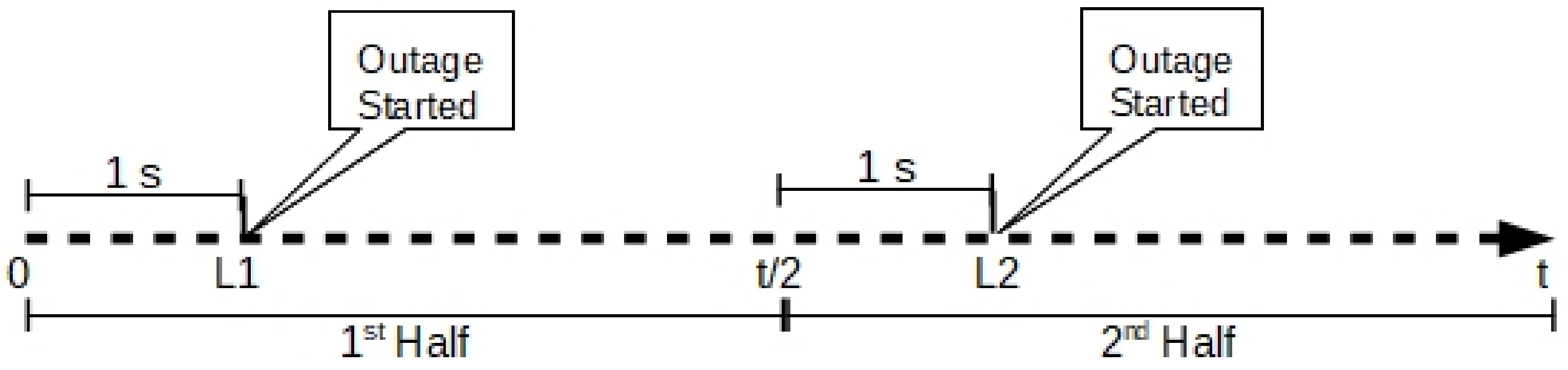
Each video was simulated with a single network outage, represented as L1 or L2 as shown in Figure 4. L1 means that the network outage occurs in the first half of the video after playing a one-second video, and L2 represents the outage location in the second half of the video after playing $t/2+1$ seconds of video. For each video, the length of network outage was either 1 s or 2 s. The videos and network outage details are given in

Table 2. Video used for subjective analysis.

Video (Motion)	Video Length t [s]	Outage Location	Outage Length [s]
Foreman (Medium)	10	L1 or L2	1 s or 2 s for L1 or L2
Football (Fast)	8	L1 or L2	1 s or 2 s for L1 or L2
News (Slow)	10	L1 or L2	1 s or 2 s for L1 or L2

.

In the presence and absence of a sending buffer, videos are simulated in two scenarios.

Table 3. Simulation parameters and their results in terms of video freeze and loss duration.

Case	${\mathit{\tau }}_{\mathbf{s}}\left[\mathbf{s}\right]$	${\mathit{\tau }}_{\mathbf{j}}\left[\mathbf{s}\right]$	${\mathit{\tau }}_{\mathbf{o}}\left[\mathbf{s}\right]$	n	${\mathit{F}}_{\mathbf{\Delta }\mathit{t}}\left[\mathbf{s}\right]$	${\mathit{L}}^{\prime }\left[\mathbf{s}\right]$
1a	0	1	1	n/a	1	1
1b	1	1	1	1	1	0
1c	1	1	1	2	0.5	0
2a	0	2	2	n/a	2	2
2b	2	2	2	1	2	0
2c	2	2	2	2	1	0

lists all simulation scenarios for all videos. We selected different simulation scenarios to test the performance of the proposed video streaming, without and with sender buffer. In Section 8, we concluded that both the sender buffer and the jitter buffer must be the same size to maximize the efficiency of the buffers, which we follow in the experiments. The first column and the second column represent the size of the sender buffer and jitter buffer in time units. The third column shows the duration of the network outage.

Obviously, when the network outage duration exceeds the jitter buffer, the user will experience video freeze and jump artifacts. However, when the network outage is shorter than the jitter buffer, the user does not see any artifacts. To reduce the complexity of discussion and experiments, we kept the network outage equal to the length of the jitter buffer and/or sender buffer. Cases 1a and 2a do not use a sender buffer. In these cases, even when the network outage is equal to the jitter buffer size, the user will face some video freeze and loss of video content. As discussed in Section 8, when a network outage is greater than the sender buffer, data loss occurs at the sender side. However, after the network outage, only the data stored in the sender buffer are of interest. Thus, to test the usefulness of the sender buffer, cases 1b, 1c, 2b, and 2c were chosen for the simulation, in which the network outage is equal to the sender buffer.

The capacity factor n is another important multiplicative factor, which helps to reduce the freeze time duration and get back the live video in a faster way. Column 4 shows the capacity factor n. The last two columns represent the freeze time, cf. Equation (47), and the data loss duration according to Equation (43)

$$L^{\prime }=\frac{L}{R_{\mathrm{sr}}}={\tau }_{\mathrm{o}}-{\tau }_{\mathrm{sj}}\mathrm{where}{\tau }_{\mathrm{o}}\ge {\tau }_{\mathrm{sj}}$$

(54)

As described in Table 3, six different simulation scenarios are used to create test videos. For each selected simulation scenario, we apply the network outage in two different locations, one in the first half of the video and the other in the other half of the video. This results in a total of 12 videos for each video sequence and a total of 36 videos for subjective testing.

The subjective tests were conducted in the perception lab of Blekinge Institute of Technology, Sweden using absolute category rating (ACR). The perception lab is designed according to the recommendation of ITU-R BT. 500 [41] and ITU-T P.910 [42]. Before starting the user rating, verbal and written instructions were provided to each participant. All participants are given the instruction “In this experiment, you are going to rate the quality of the video regardless of the content of the video. Please be considerate about your judgment and remember there is not an exact score for a video. It is an opinion and can vary from person to person”. After viewing each video, participants are asked “Please rate the quality of this video”. A total of 46 subjects participated in this study and gave feedback on the video quality using the single stimulus method on the 5-point Absolute Category Rating (ACR) scale with categories 1 = bad, 2 = poor, 3 = fair, 4 = good, and 5 = excellent. All test videos have artifacts like freeze, jump, and miss, so a certain spread of the users’ ratings was expected, along with some rather low user ratings. However, the feedback of three participants was different. One of them had given score 5 to all videos. Most of the feedback of two other users fall outside the interval obtained from applying the Interquartile range (IQR), so they were considered as outliers. Thus, 43 participant ratings were analyzed further.

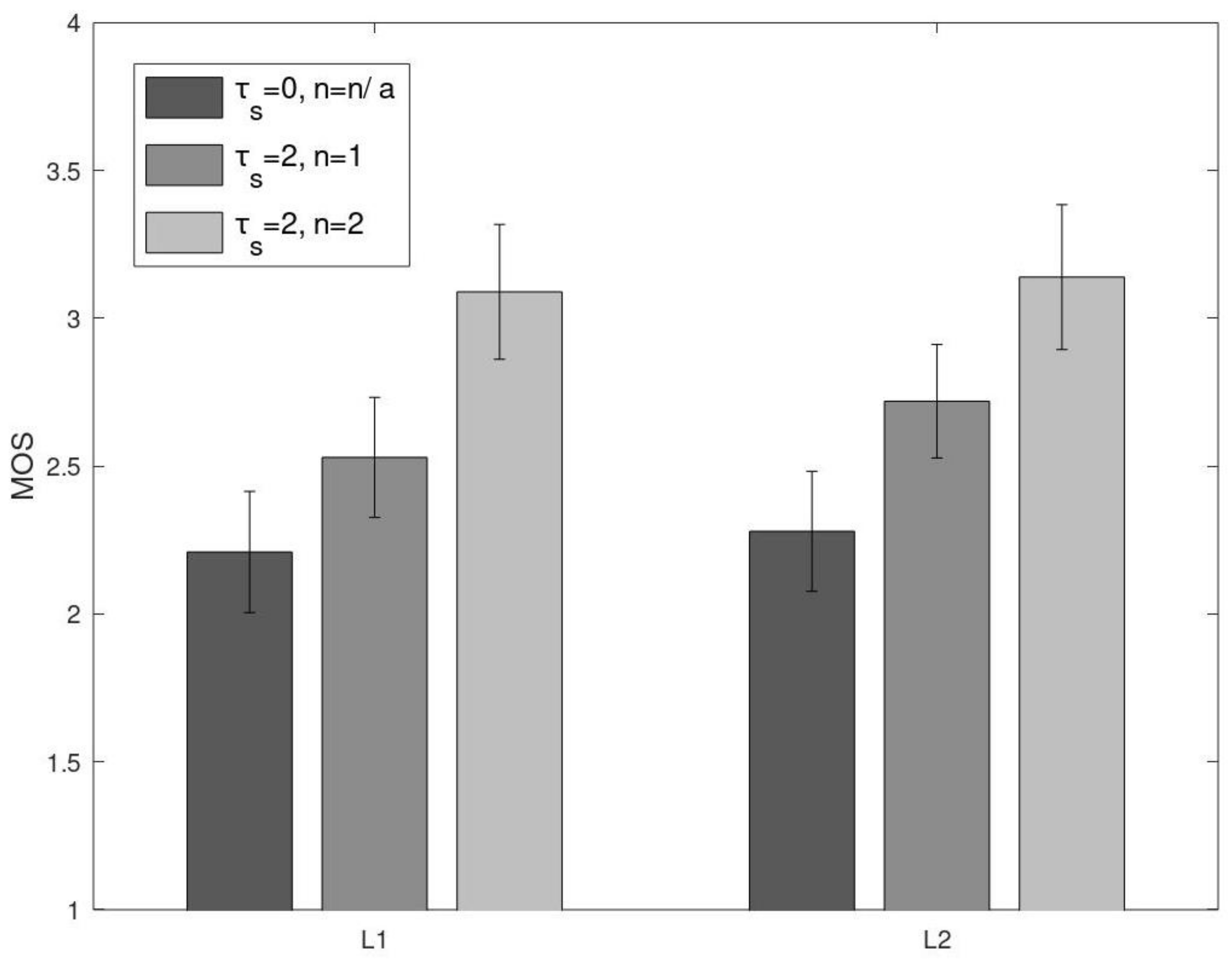
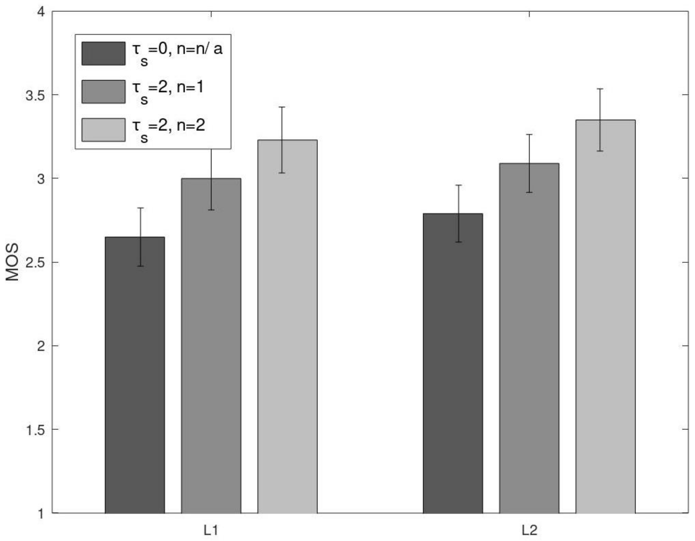
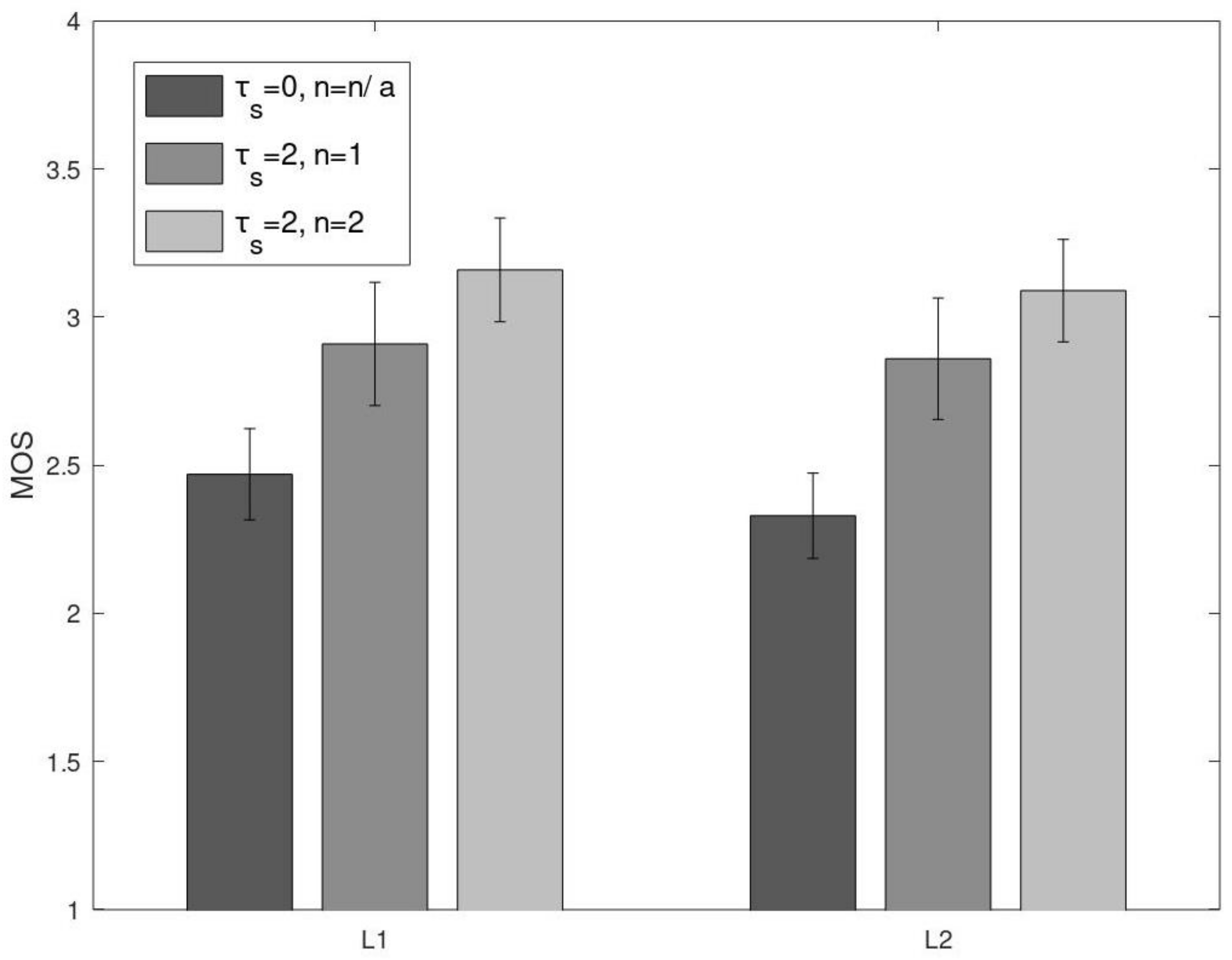
Figure 5 and Figure 6 show the user ratings for the “Foreman” video simulated with and without the sender buffer, and the corresponding network outages. The abscissa indicates the outage location in the video, and the ordinate shows the Mean Opinion Score (MOS).

In the absence of the sender buffer (${\tau }_{\mathrm{s}}=0$), the network outage results in video freeze-and-jump. From Table 3, we can see that, in the absence of the sender buffer, the video loss and video freeze are equal to the outage duration. Users react to these artifacts and rate the video on average below 2.5. This user rating applies to both ${\tau }_{\mathrm{o}}=2$ and ${\tau }_{\mathrm{o}}=1$. However, average user ratings for ${\tau }_{\mathrm{o}}=2$ are lower than average users’ ratings for ${\tau }_{\mathrm{o}}=1$, which is obvious, as the users faced longer video losses and video freezes. Moreover, it is also observed that the user ratings vary with respect to the location of video under similar artifacts. Similar reactions are observed and reported by the authors in [15,16]. The presence of the sender buffer helps to save the data during the network outage. As a result, it mitigates the video artifacts like freeze, jump, and miss as observed during the experiments and shown in

Table 4. Simulation details and MOS for various videos (with * denoting n/a).

Simulation Parameters							Foreman	Football	News
$\mathbf{Outage}$ $\mathbf{Postion}$	${\mathit{\tau }}_{\mathbf{s}}$ $\left[\mathbf{s}\right]$	${\mathit{\tau }}_{\mathbf{j}}$ [s]	${\mathit{\tau }}_{\mathbf{o}}$ [s]	$\mathit{n}$	${\mathit{F}}_{\Delta \mathit{t}}$ [s]	$\mathit{L}$ [s]	MOS	MOS	MOS
Original							4.57 ± 0.187	4.30 ± 0.230	4.35 ± 0.256
L1	0	1	1	*	1	1	2.44 ± 0.202	2.60 ± 0.164	2.70 ± 0.182
L2	0	1	1	*	1	1	2.49 ± 0.224	2.67 ± 0.159	2.60 ± 0.189
L1	0	2	2	*	2	2	2.21 ± 0.205	2.44 ± 0.153	2.47 ± 0.154
L2	0	2	2	*	2	2	2.28 ± 0.203	2.56 ± 0.167	2.33 ± 0.144
L1	1	1	1	1	1	0	3.09 ± 0.228	3.00 ± 0.188	3.16 ± 0.175
L2	1	1	1	1	1	0	3.14 ± 0.245	3.09 ± 0.173	3.09 ± 0.173
L1	1	1	1	2	0.5	0	3.37 ± 0.240	3.23 ± 0.197	3.44 ± 0.167
L2	1	1	1	2	0.5	0	3.44 ± 0.153	3.35 ± 0.186	3.40 ± 0.211
L1	2	2	2	1	2	0	2.53 ± 0.203	2.72 ± 0.153	2.91 ± 0.208
L2	2	2	2	1	2	0	2.72 ± 0.192	2.81 ± 0.152	2.86 ± 0.205
L1	2	2	2	2	1	0	3.09 ± 0.228	3.00 ± 0.188	3.16 ± 0.175
L2	2	2	2	2	1	0	3.14 ± 0.245	3.09 ± 0.173	3.09 ± 0.173

as well as in Figure 5 and Figure 6. The sender buffer of length 1 s (${\tau }_s=1$) helps to improve MOS from 2.44 to 3.55, while an extended length to 2 s (${\tau }_s=2$) makes MOS improve from 2.21 to 2.72. Figure 5 and Figure 6 illustrate that MOS values increase from 3.09 and 3.14 for $n=1$ and from 3.37 and 3.55 for $n=2$ when increasing ${\tau }_s={\tau }_j={\tau }_o=1$ to ${\tau }_s={\tau }_j={\tau }_o=2$. Obviously, an increase in the data rate after network outage in the presence of the sender buffer also improves the user ratings.

Figure 7, Figure 8, Figure 9 and Figure 10 show the average user ratings for “Football” and “News”, respectively. These bar charts for “Football” and “News” are depicting similar behaviors as the “Foreman” videos.

Table 4 shows the detailed MOS results of the "Foreman”, "Football”, and “News” videos.

The average user ratings of the original videos “Foreman”, “Football”, and “News” are 4.57, 4.30, and 4.35, respectively. This indicates that the users did not rank the original video as excellent, and the user ratings vary from video to video. This behavior was also reported in a previous study [8]. From the results, we can see that this random behavior is also found in the average user rating of all videos. From Table 4, we can realize that the network outage (${\tau }_o=1$) degrades the average user ratings from good to poor. However, for the same network outage settings, the sender buffer helps to improve the average user ratings from poor to fair.

9.1. Analysis of the Impact of the Sender Buffer

From the above results, the MOS of videos streamed with the sender buffer (${\mu }_1$) is apparently better than the MOS of video streamed without the sender buffer (${\mu }_2$) under otherwise similar conditions. To confirm that ${\mu }_1$ is significantly different and greater than ${\mu }_2$, Student’s t-test was used (as implemented in R). The null hypothesis is defined as

$$H_0:{\mu }_1\le {\mu }_2$$

(55)

Moreover, to calculate how much MOS is augmented due to the sender buffer, we also computed the MOS gain

$$\Delta \mathrm{MOS}={\mu }_1-{\mu }_2$$

(56)

Table 5. Analysis of the impact of the sender buffer using Student’s t-test.

Foreman
OL	${\tau }_{\mathrm{j}}={\tau }_{\mathrm{o}}$ = 1						${\tau }_{\mathrm{j}}={\tau }_{\mathrm{o}}$ = 2
	n	MOS ${\tau }_{\mathrm{s}}={\tau }_{\mathrm{j}}$	MOS ${\tau }_{\mathrm{s}}=0$	$\Delta \mathrm{MOS}$	p-value $\alpha =0.05$	H0 ${\mu }_1\le {\mu }_2$	MOS ${\tau }_{\mathrm{s}}={\tau }_{\mathrm{j}}$	MOS ${\tau }_{\mathrm{s}}=0$	$\Delta \mathrm{MOS}$	p-value $\alpha =0.05$	H0 ${\mu }_1\le {\mu }_2$
L1	1	3.09	2.44	0.65	$1.2\times {10}^{-5}$	Reject	2.53	2.21	0.33	$7.3\times {10}^{-3}$	Reject
L2	1	3.14	2.49	0.65	$3.8\times {10}^{-5}$	Reject	2.72	2.28	0.44	$2.4\times {10}^{-4}$	Reject
L1	2	3.37	2.44	0.93	$1.1\times {10}^{-7}$	Reject	3.09	2.21	0.88	$1.6\times {10}^{-7}$	Reject
L2	2	3.44	2.49	0.95	$3.2\times {10}^{-10}$	Reject	3.14	2.28	0.86	$6.9\times {10}^{-9}$	Reject
Football
OL	${\tau }_{\mathrm{j}}={\tau }_{\mathrm{o}}$ = 1						${\tau }_{\mathrm{j}}={\tau }_{\mathrm{o}}$ = 2
	n	MOS ${\tau }_{\mathrm{s}}={\tau }_{\mathrm{j}}$	MOS ${\tau }_{\mathrm{s}}=0$	$\Delta \mathrm{MOS}$	p-value $\alpha =0.05$	H0 ${\mu }_1\le {\mu }_2$	MOS ${\tau }_{\mathrm{s}}={\tau }_{\mathrm{j}}$	MOS ${\tau }_{\mathrm{s}}=0$	$\Delta \mathrm{MOS}$	p-value $\alpha =0.05$	H0 ${\mu }_1\le {\mu }_2$
L1	1	3.00	2.60	0.40	$1.9\times {10}^{-3}$	Reject	2.72	2.44	0.28	$4.4\times {10}^{-3}$	Reject
L2	1	3.09	2.67	0.42	$8.2\times {10}^{-5}$	Reject	2.81	2.56	0.26	$7.3\times {10}^{-3}$	Reject
L1	2	3.35	2.60	0.74	$6.4\times {10}^{-9}$	Reject	3.00	2.44	0.56	$2.5\times {10}^{-6}$	Reject
L2	2	3.23	2.67	0.56	$2.5\times {10}^{-6}$	Reject	3.09	2.56	0.53	$5.4\times {10}^{-6}$	Reject
News
OL	${\tau }_{\mathrm{j}}={\tau }_{\mathrm{o}}$ = 1						${\tau }_{\mathrm{j}}={\tau }_{\mathrm{o}}$ = 2
	n	MOS ${\tau }_{\mathrm{s}}={\tau }_{\mathrm{j}}$	MOS ${\tau }_{\mathrm{s}}=0$	$\Delta \mathrm{MOS}$	p-value $\alpha =0.05$	H0 ${\mu }_1\le {\mu }_2$	MOS ${\tau }_{\mathrm{s}}={\tau }_{\mathrm{j}}$	MOS ${\tau }_{\mathrm{s}}=0$	$\Delta \mathrm{MOS}$	p-value $\alpha =0.05$	H0 ${\mu }_1\le {\mu }_2$
L1	1	3.16	2.70	0.47	$2.1\times {10}^{-5}$	Reject	2.91	2.47	0.44	$1.5\times {10}^{-4}$	Reject
L2	1	3.09	2.60	0.49	$7.4\times {10}^{-5}$	Reject	2.86	2.33	0.53	$9.2\times {10}^{-5}$	Reject
L1	2	3.44	2.70	0.74	$9.8\times {10}^{-12}$	Reject	3.16	2.47	0.70	$4.1\times {10}^{-9}$	Reject
L2	2	3.40	2.60	0.79	$7.5\times {10}^{-9}$	Reject	3.09	2.33	0.77	$2.1\times {10}^{-11}$	Reject

shows the Student’s t-test results along with the MOS gain. Results are grouped for ${\tau }_{\mathrm{j}}={\tau }_{\mathrm{o}}=1$ and ${\tau }_{\mathrm{j}}={\tau }_{\mathrm{o}}=2$ for each video. Columns 5 and 9 show the MOS gain, whereas columns 7 and 11 are based on the outcome of the null hypothesis. The MOS gain is always greater than zero, which supports the assumption that the presence of a sender buffer helps to improve the MOS.

From Table 5, we can see that the null hypothesis is rejected in all cases. As in columns 6 and 10, we can see that all p-values are much smaller than $\alpha =0.05$. Hence, the conclusion is that MOS with a sender buffer is greater than the MOS without the sender buffer, which implies that the sender buffer minimizes the effects of network outages and improves the user experience.

9.2. Analysis of the Impact of the Capacity Factor n on MOS Gain

To examine the role of the capacity factor (n) on MOS in the presence of sender buffer, we analyze MOS for $n=2$ denoted by ${\mu }_1(n=2)$ and MOS for $n=1$ denoted by ${\mu }_2(n=1)$ under otherwise similar conditions, to substantiate that the bigger capacity factor n better mitigates the impact of the network outage. The Student’s t-test was used with the following null hypothesis:

$$H_0:{\mu }_1(n=2)\le {\mu }_2(n=1)$$

(57)

In order to calculate how much MOS is increased due to the capacity factor (n) in the presence of the sender buffer, the MOS gain is calculated as

$$\Delta \mathrm{MOS}={\mu }_1(n=2)-{\mu }_2(n=1)$$

(58)

In

Table 6. Analysis of the impact of the capacity factor n on the MOS Gain using Student’s t-test.

Foreman
OL	${\tau }_{\mathrm{j}}={\tau }_{\mathrm{s}}={\tau }_{\mathrm{o}}=1$					${\tau }_{\mathrm{j}}={\tau }_{\mathrm{s}}={\tau }_{\mathrm{o}}=2$
	MOS $n=2$	MOS $n=1$	$\Delta \mathrm{MOS}$	p-value $\alpha =0.05$	H0 ${\mu }_1\le {\mu }_2$	MOS $n=2$	MOS $n=1$	$\Delta \mathrm{MOS}$	p-value $\alpha =0.05$	H0 ${\mu }_1\le {\mu }_2$
L1	3.37	3.09	0.28	$1.1\times {10}^{-2}$	Reject	3.09	2.53	0.56	$5.2\times {10}^{-5}$	Reject
L2	3.44	3.14	0.30	$8.8\times {10}^{-3}$	Reject	3.14	2.72	0.42	$1.2\times {10}^{-3}$	Reject
Football
OL	${\tau }_{\mathrm{j}}={\tau }_{\mathrm{s}}={\tau }_{\mathrm{o}}=1$					${\tau }_{\mathrm{j}}={\tau }_{\mathrm{s}}={\tau }_{\mathrm{o}}=2$
	MOS $n=2$	MOS $n=1$	$\Delta \mathrm{MOS}$	p-value $\alpha =0.05$	H0 ${\mu }_1\le {\mu }_2$	MOS $n=2$	MOS $n=1$	$\Delta \mathrm{MOS}$	p-value $\alpha =0.05$	H0 ${\mu }_1\le {\mu }_2$
L1	3.23	3.00	0.23	$4.3\times {10}^{-2}$	Reject	3.00	2.72	0.28	$1.6\times {10}^{-2}$	Reject
L2	3.35	3.09	0.26	$2.0\times {10}^{-2}$	Reject	3.09	2.81	0.28	$1.1\times {10}^{-2}$	Reject
News
OL	${\tau }_{\mathrm{j}}={\tau }_{\mathrm{s}}={\tau }_{\mathrm{o}}=1$					${\tau }_{\mathrm{j}}={\tau }_{\mathrm{s}}={\tau }_{\mathrm{o}}=2$
	MOS $n=2$	MOS $n=1$	$\Delta \mathrm{MOS}$	p-value $\alpha =0.05$	H0 ${\mu }_1\le {\mu }_2$	MOS $n=2$	MOS $n=1$	$\Delta \mathrm{MOS}$	p-value $\alpha =0.05$	H0 ${\mu }_1\le {\mu }_2$
L1	3.44	3.16	0.28	$4.4\times {10}^{-3}$	Reject	3.16	2.91	0.26	$1.3\times {10}^{-2}$	Reject
L2	3.40	3.09	0.30	$1.1\times {10}^{-2}$	Reject	3.09	2.86	0.23	$2.9\times {10}^{-2}$	Reject

, the impact of the capacity factor n is illustrated by the MOS gain in columns 4 and 9, all with positive values. Column 5 and 10 revealed the p-values of the Student’s t-test applied on the MOS for $n=2$ and MOS for $n=1$. As all p-values are less than 0.05, we can reject the null hypothesis. Both MOS gain and Student’s t-test show that a bigger capacity factor n in the presence of a sender buffer helps to mitigate the impact of the network outage in a better way through reduced video freeze durations, which obviously improves the QoE.

9.3. Limitations Regarding Resolutions

The experiments were performed using low-end QVGA resolution, which may appear outdated at least in the wealthy economies, while 3G is still standard in developing countries, or offered as low-cost alternative even in the developed countries.

The questions arise regarding what to expect from a higher resolution. At a higher resolution, an outage of a certain duration will naturally affect more packets. However, in our work, the duration of the outage, as compared to sender and jitter buffer, is the key parameter.

As expected, high-resolution videos yield better subjective ratings in terms of MOS [43] or objective Video Quality Metric (VQM) and Structural Similarity Index Measure (SSIM) values [44], as compared to low-resolution videos. In Reference [16], the authors studied the effects of video freezes with resolutions (QCIF, CIF, QVGA, and VGA), and compared MOS ratings with the Temporal Quality Metric (TQM) and Perceptual Evaluation of Video Quality (PEVQ) values. They found that video resolutions played a minor role on both subjective and objective video quality ratings. However, it remains to be investigated to which extent a high streaming resolution (such as 4K) would affect the ratings of the temporal disturbances.

10. Conclusions

In live streaming, network outage may result in video freezes, jumps, or misses. Subjective studies showed that artifacts like freeze-and-jump degrade the video QoE. To mitigate the degradation of the QoE, a sender buffer-based solution was proposed.

Analytically, we have discussed that the sender buffer helps in reducing the data loss and freeze time duration during the network outage. The possibility to flush the sender buffer data with a higher data rate on the availability of the channel can reduce the freeze time duration even further. The relationship between the size of the sender buffer and receiver buffer was also analyzed in terms of various parameters. It was found that the size of both buffers should be equal for the optimal result.

Subjective tests were also conducted for the videos exposed to the network outage during the transmission. It is found that the user rating improves a lot in the presence of sender buffer, especially with a higher capacity factor ($n>1$). Based on both our analytical and simulation-based user study, we may conclude that using a well-dimensioned sender buffer in combination with a faster-than-needed channel helps to mitigate the effect of the network outages on the video QoE.

In our future work, we plan to investigate the role of a backup buffer at the receiver, in parallel to the jitter buffer. During our work, so far, we have observed that it is very difficult to minimize the freeze time so that the user cannot feel it. In order to remove this minimum freeze time from the user display, we are investigating the concept of a backup buffer in parallel to the jitter buffer at the receiving side, which is be used to replay contents when the jitter buffer is empty in order to keep the user involved.

We are also considering ways to detect and inform the sender about the network outage, as quickly as possible. Furthermore, we are also interested in optimising the usage of the available link capacity after the network outage in the presence of other streams, and for various combinations of resolutions and mobile network connectivity.