Multi-Input Deep Learning Based FMCW Radar Signal Classification

Abstract

In autonomous driving vehicles, the emergency braking system uses lidar or radar sensors to recognize the surrounding environment and prevent accidents. The conventional classifiers based on radar data using deep learning are single input structures using range–Doppler maps or micro-Doppler. Deep learning with a single input structure has limitations in improving classification performance. In this paper, we propose a multi-input classifier based on convolutional neural network (CNN) to reduce the amount of computation and improve the classification performance using the frequency modulated continuous wave (FMCW) radar. The proposed multi-input deep learning structure is a CNN-based structure using a distance Doppler map and a point cloud map as multiple inputs. The classification accuracy with the range–Doppler map or the point cloud map is 85% and 92%, respectively. It has been improved to 96% with both maps.

1. Introduction

Recently, autonomous driving technologies such as the advanced driver assistance system (ADAS) are being actively. ADAS are commercially available to reduce drivers’ fatigue and help safe driving. ADAS includes the adaptive cruise control, intelligent parking assist system, lane departure warning system and autonomous emergency braking system [1,2,3]. Among them, the autonomous emergency braking system prevents accidents by directly operating the brake when an accident such as the collision is expected. To prevent accidents, it is important to be aware of the surrounding environment.

Sensors such as cameras, lidar sensors and radars are used to recognize the surrounding environment. Cameras are inexpensive and have the advantage of being able to recognize objects on the road, but distance information cannot be obtained. Lidar sensors are expensive and have the disadvantage of not getting good performance in any weather conditions such as snow or rain. Radars can measure distance and speed [4], but have the disadvantage of less capable of distinguishing objects than lidar sensors [5]. However, compared to cameras and lidar sensors, they have a more robust detection performance in dark and bad weather conditions [5]. Therefore, radars have emerged as one of the core sensors for ADAS to replace cameras and expensive lidar sensors that are highly affected by the surrounding environment, and research on implementing target classifiers using deep learning-based radars are actively underway [6,7,8].

Many studies [9,10,11,12] use a single input such as the spectrogram and range–Doppler map for classification. However, these images change greatly depending on the angle at which the object faces the radar. Additionally, there are many similar images between objects to be identified. These similar images degrade the identification accuracy of cars, people and motorcycles. The point cloud map is easier to identify objects because the image difference between objects is clearer than the range–Doppler map.

In this paper, we use two features of the range–Doppler and point cloud maps to improve identification performance with deep learning systems. There are no common features between the range–Doppler and point cloud maps except the intensity of the reflected signal. Therefore, when the two features are directly putting into a deep learning system as in Figure 1, optimal performance cannot be obtained.

The contributions of the paper are summarized as follows:

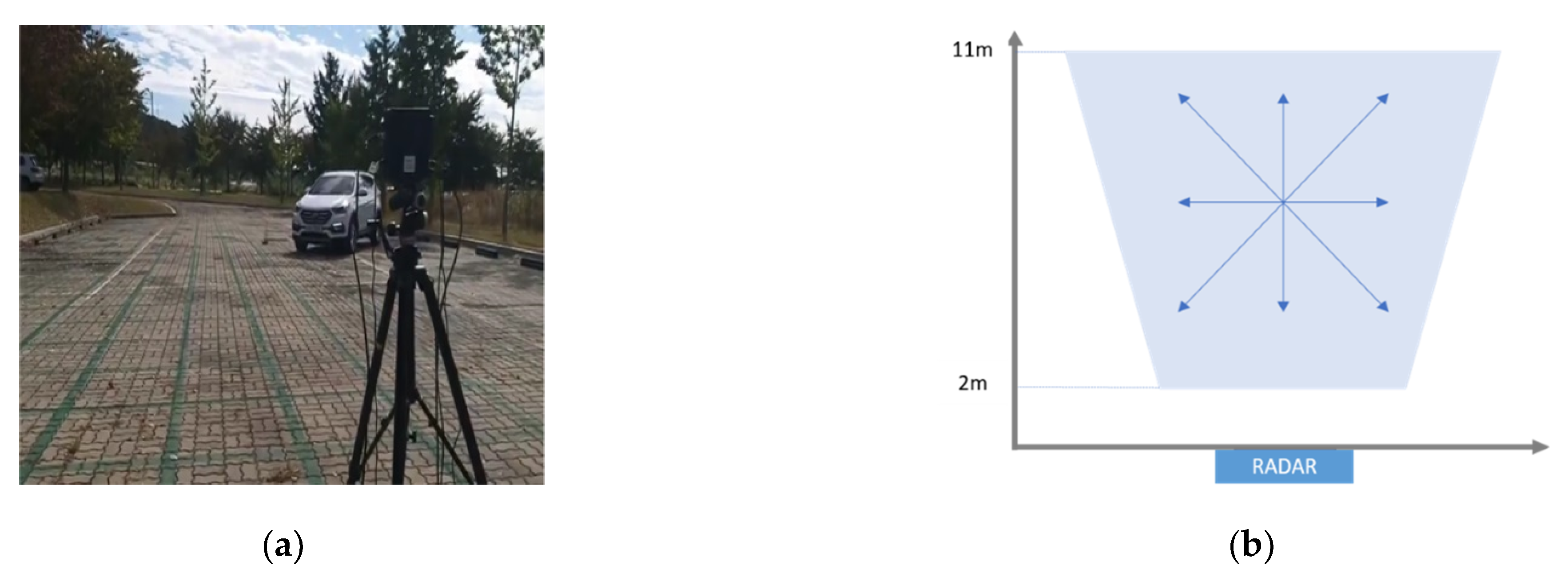
• We propose a radar-based classification system with collected data using frequency modulated continuous wave (FMCW) radar.
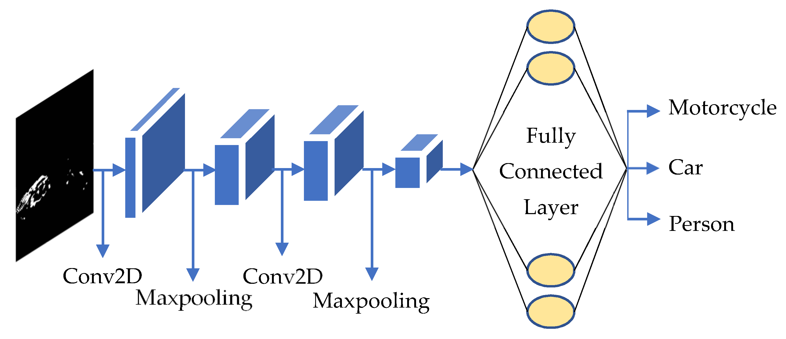
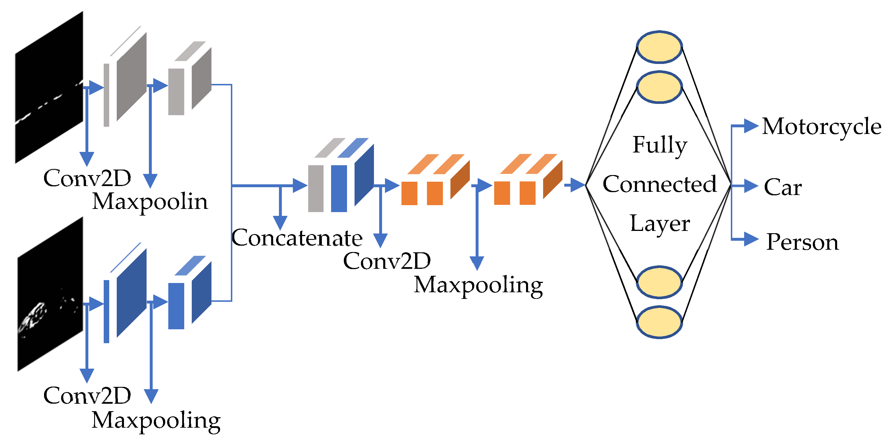
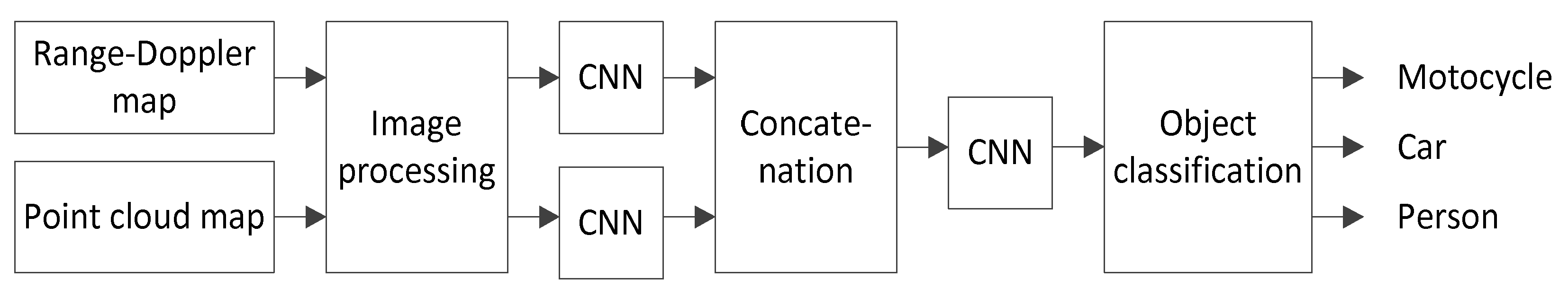
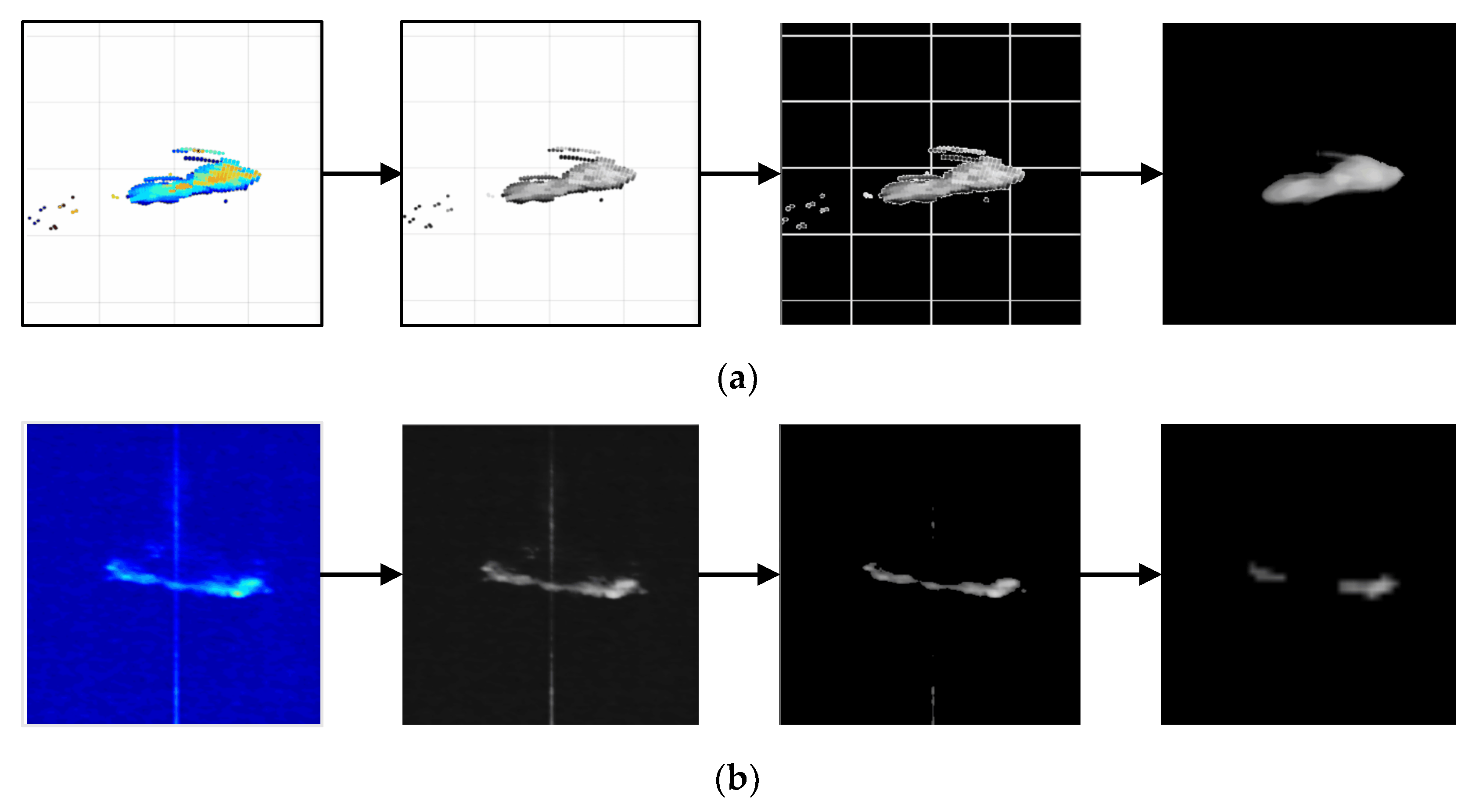
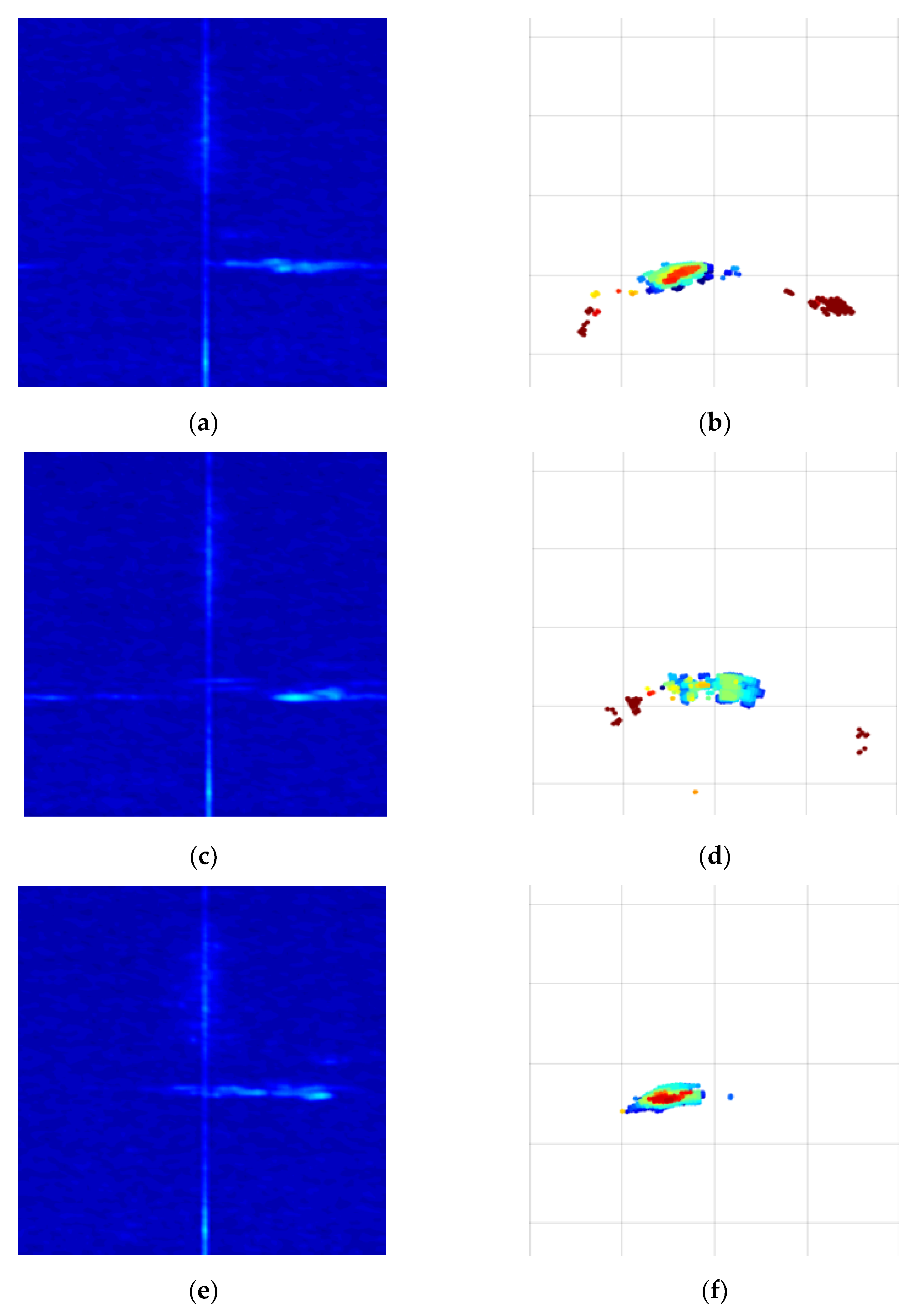
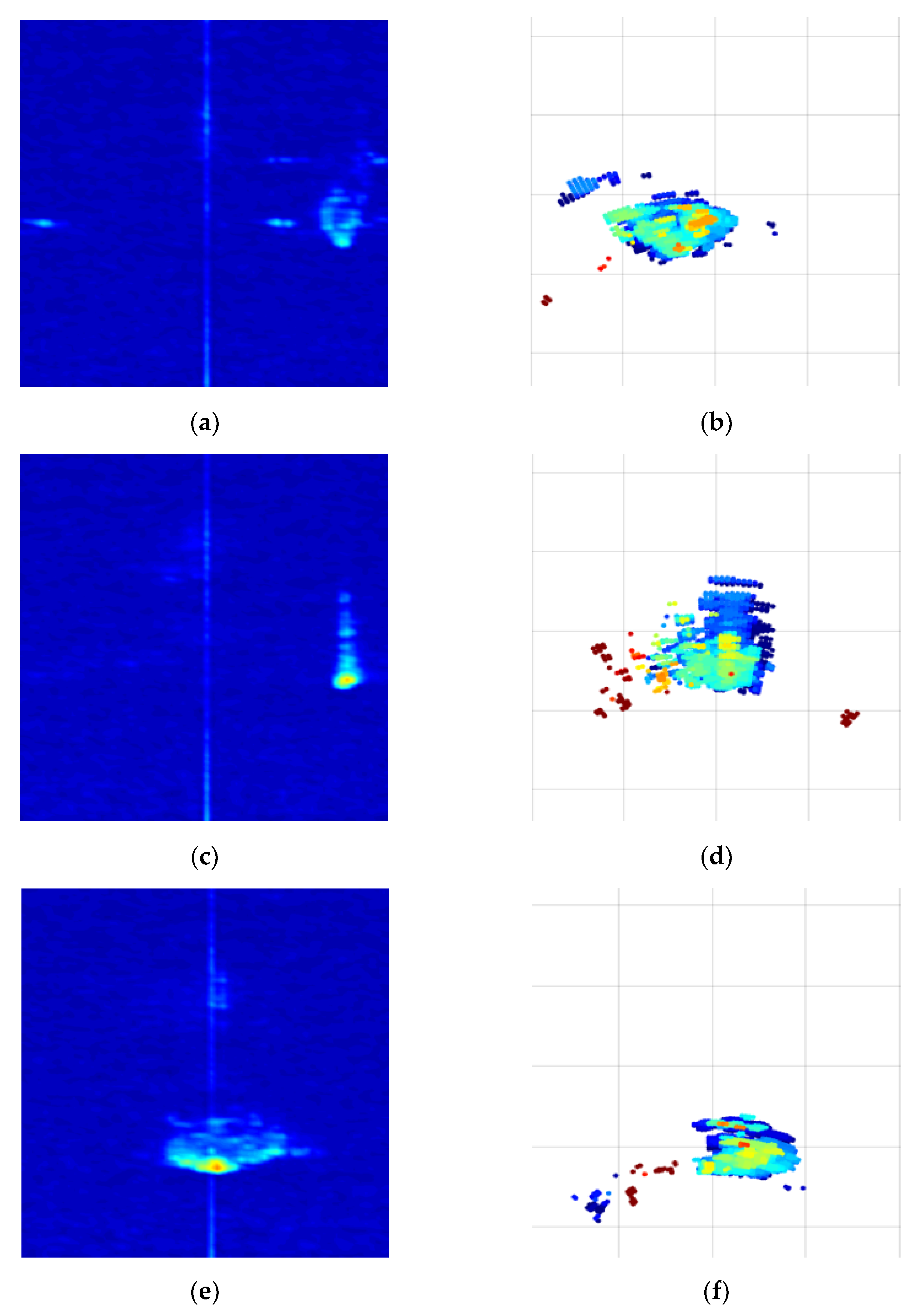
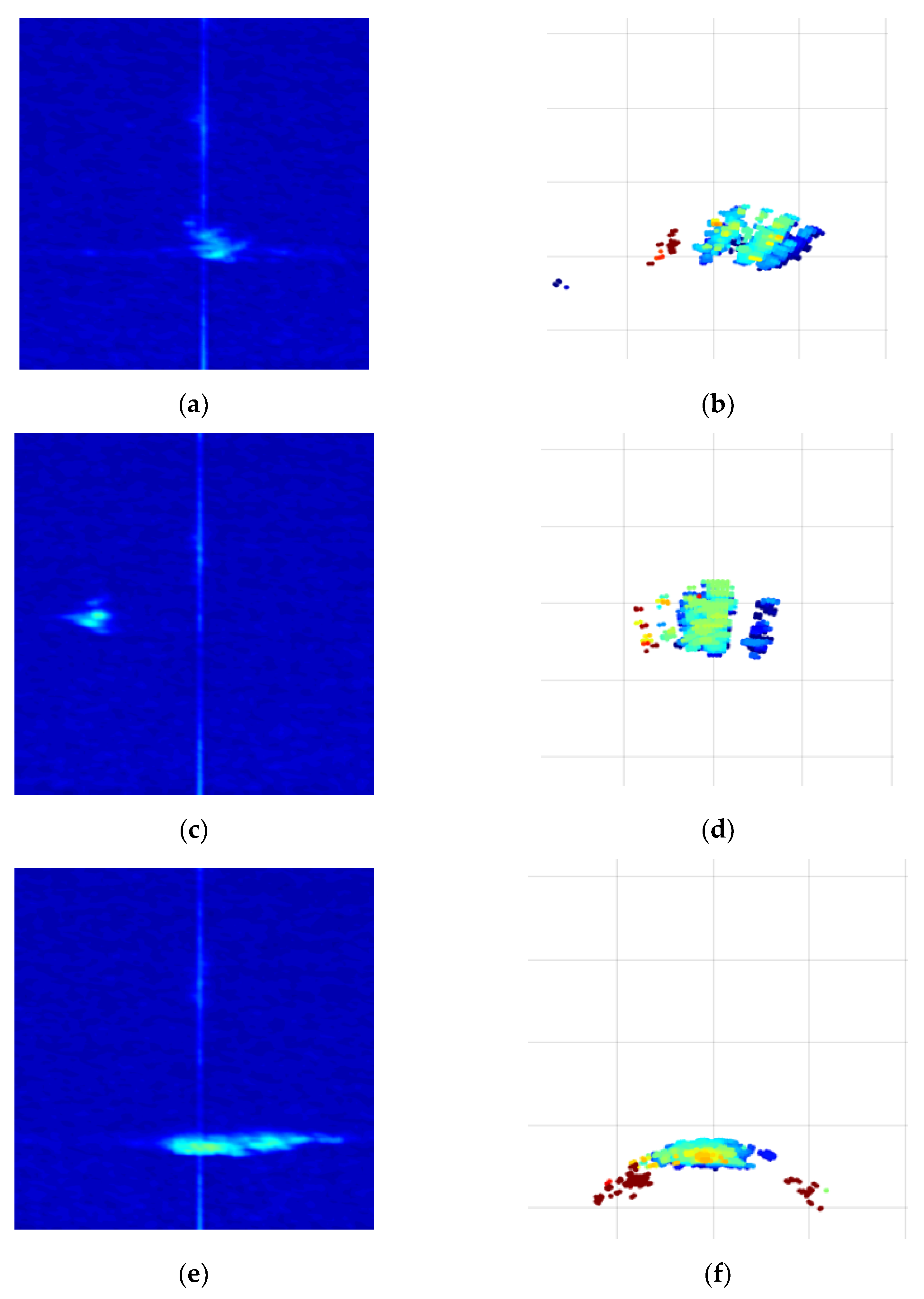
• The distance–Doppler map changes greatly depending on the angle at which the object faces the radar. Therefore, we propose a convolutional neural network (CNN) -based multi-input deep learning model, which uses both the distance–Doppler map and the point cloud map as inputs to enhance the classification accuracy.

The rest of the paper is organized as follows. Section 2 describes related work on the object classification algorithms using radars. Section 3 presents the conventional single-input CNN structure and proposes a multiple-input CNN structure. Section 4 discusses the data collection method and the data analysis, and Section 5 explains the experimental results using the collected data. Finally, we conclude in Section 6.

2. Related Work

In general, the radar cross section [13], phase information [14] and micro-Doppler [15,16] are used to classify objects using radar. However, conventional object detection and classification methods require a large computational complexity [17]. To resolve this problem, a classification technique applying deep learning using an FMCW radar has been proposed in recognition of human behavior and hand gestures. Vaishnav et al. [18] proposed a human behavior recognition technique using an FMCW radar. Additionally, Anishchenko et al. [19] proposed a non-contact automatic fall detection system with an AlexNet using radar data. Skaria et al. [20] used a three-channel time–Doppler map data to improve the performance of the conventional classifier using data from one channel and showed an improved performance of about 10% compared to the conventional single-channel range–Doppler map. Kim et al. [21] created a time–Doppler spectrogram using a 7.25 GHz Doppler radar. Additionally, then, deep convolutional neural networks (DCNNs) were used to detect the presence and behavior of humans.

Identification research using radar has been applied not only to human behavior recognition but also in various fields such as autonomous vehicles and active sonar. Angelov et al. [22] used automotive radar data and presented the results of classifying cars, people and bicycles using three artificial neural network structures: a convoluted network, a residual network and a combination of the convolutional and recurrent network. Lee et al. [23] used CNN as an identifier using power-normalized Cepstral coefficients (PNCC) as a feature for the identification of underwater objects in the active sonar. Daher et al. [24] identified various classes based on Rulex [25], a high-performance machine learning package, using 24 GHz radar data. Forecasts with a varying number of classes were performed with one, two, or three classes of vehicles and one for humans. Furthermore, they applied a single forecast for all four classes and cascading forecasts in a treelike structure while varying algorithms, cascading the block order, setting class weights and varying the data splitting ratio for each forecast to improve prediction accuracy. Kim et al. [26] used CNN [27], VGG16 [28] and VGG19 [28] as feature extractors using a spectrogram, and used the support vector machine (SVM) for classification. Additionally, Kim et al. [17] analyzed the classification results according to the deep learning technique of various structures using the range–Doppler map.

Until now, most studies have changed the deep learning structure using one feature such as the spectrogram or range–Doppler map. However, since these studies make the structure of deep learning deeper, the amount of computation increases. Additionally, if only the range–Doppler map is used for identification, similar images exist between objects, or various images depending on the azimuth angle between the object and the radar will degrade the identification result.

In this paper, a basic CNN structure composed of a convolution layer and a pooling layer is used in consideration of computational complexity to resolve these problems. To solve the problem when only one range–Doppler map is used, two images are used with the distance–Doppler and point cloud maps. In addition, we propose a multiple input-based CNN identification technique to have optimal identification performance.

3. Proposed Multi-Input Based CNN Classifier

This section describes the structure of a single input CNN used for image identification and proposes a multiple input CNN structure. In all experiments, the most basic CNN structure was used considering the amount of computation. Figure 1 show the conventional data input method, the deep learning structure and output used in the experiment. Figure 2 shows the proposed multi-input-based deep learning structure. The conventional CNN structure used for image identification uses single channel or two-channel data as a single input as shown in Figure 1. Additionally, based on a single input, CNN and long short-term memory (LSTM) are combined and used in combination with deep learning of several structures [29].

We used the deep learning structure in Figure 1 for identification using 1-channel and 2-channel images. The point cloud map has a relatively uniform image than the range–Doppler map. Therefore, better classification performance can be obtained when the range–Doppler map and the point cloud map are used together. However, there is no common factor between the two maps because we imaged to consider only the shape of the object in the two maps for object identification, optimal performance cannot be obtained when a two-channel image is used as an input. As shown in Figure 2, features are extracted from the range–Doppler map and the point cloud map by using CNN. Figure 3 shows the block diagram of the proposed algorithm.

The first step of proposed algorithm is image preprocessing. In Figure 4a is the preprocessing of the point cloud map with x and y labels removed, and Figure 4b is the preprocessing of the range–Doppler map. The preprocessing applied to both images is the same, and both images use an image with a resolution of $50\times 50$ to shorten the learning time. Both the range–Doppler map and the point cloud map are represented in color according to the intensity of the signal. In the case of a range–Doppler map, a signal due to noise exists even in a part where an object does not exist. Additionally, in the case of the point cloud map, even if the signal reflected by the same object has a similar shape, the signal intensity decreases as the distance increases. Therefore, to reduce the influence of the noise signal and use only the shape of the object generated by the reflected signal for learning, the RGB channel is converted to a gray channel. Afterwards, to completely remove the grids and noise, a threshold value is set to 253, noise signals lower than the intensity of the reflected signal are removed, and a median filter is applied.

The next step is feature extraction. Features are extracted by CNN. Features extracted from each of the distance–Doppler and point cloud maps are concatenated into one. Afterward, features are extracted once more from the concatenated data. Finally, the object is classified using a fully connected layer.

4. Experiment Setup and Data Analysis

This section describes the experimental scenario for acquiring data directly from the radar, the image preprocessing for deep learning and analyzes the characteristics of each object image. A 79 GHz-band FMCW radar was used, and the specifications of the radar are shown in

Table 1. Radar specification.

Parameter	Value
Center frequency	79 GHz
Bandwidth	2 GHz
Resolution	Vertical and horizontal ${3.8}^{\circ }$
Field of view	Vertical and horizontal ${90}^{\circ }$

.

The radar was installed at a height of 1.5 m, and the experiment was conducted in a space with no objects other than the objects to be tested as shown in Figure 5a. The cars used in the experiment are Hyundai Santafe and Chrysler 300c, and the motorcycle is SYM GTS125i. Figure 5b shows the path traveled by the targets. The radar on the x-axis is the location where the radar is installed, and the square is the radar detection range. Cars have stronger reflected signals than humans, so they can be detected even at the maximum radar detection distance of 12 m. However, since it is difficult to detect a person with weak reflected signal strength, the maximum distance is limited to 11 m, and the experiment was not conducted at 0–2 m due to the strong reflected wave. So, all targets moved within 2–11 m, and the targets moved vertically, horizontally and diagonally as shown by the arrows in Figure 5b to collect data from various angles. People data used 1746 and 416 data for training and verification, respectively, and 1648 and 411 data for cars and 1604 and 441 data for the motorcycle were used in the experiment.

Figure 6a,c,e represents the range–Doppler map when a person moves in the diagonal, vertical and horizontal directions, respectively, the x-axis represents the Doppler, and the y-axis represents the range. Regardless of the direction of movement, the reason that the Doppler value appears in the form of a wide spread in positive and negative values is due to the reflected signal caused by shaking of arms and legs when walking. Point cloud maps of Figure 6b,d,f shows similar images regardless of direction except for the surrounding noise signals. As shown in Figure 6, the distance Doppler map by a person has various types of images depending on the walking speed, that is, the speed at which the arms and legs shake.

Figure 7 shows an image of a car moving diagonally, vertically and transversely from the top.

Figure 7a,c,e represents the range–Doppler map when the vehicle moves in the diagonal, vertical and horizontal directions, respectively. When a person moved, the intensity of the reflected signal was stronger compared to the range–Doppler map. In the case of Figure 7a,e, the range–Doppler map had a more diverse Doppler value when moving in the vertical direction due to the wheel and wheel movement. Additionally, the reason Figure 7e had a wider Doppler value than Figure 7a is that the area of the wheel viewed by the radar is wider. However, as shown in Figure 7c, when the car approached or moved away from the radar, the Doppler value was fixed and spread up and down in the graph. In the case of the point cloud map, it appeared long in the direction the car was moving.

Figure 8 shows the data when the motorcycle is moving. Figure 8a,b is the range–Doppler map and point cloud map when moving in the diagonal direction, respectively, and in the case of the range–Doppler map, it can be seen that the Doppler value generated by the wheel appeared weakly around a strong signal. The point cloud map spread diagonally like a motorcycle. Figure 8c,d are graphs of the motorcycle moving in the radar direction, and show similar shapes to those of the vehicle in Figure 7c when moving in the vertical direction. However, it is shorter in y-axis compared to the car. The point cloud map spreads widely in the direction of movement. When moving in the transverse direction as shown in Figure 8e,f, the area where the wheel faces the radar is larger than in the diagonal direction, so it can be confirmed that more Doppler occurs than when moving in the diagonal direction. Likewise, it can be seen that the point cloud map spreads widely in the horizontal direction, which is the moving direction.

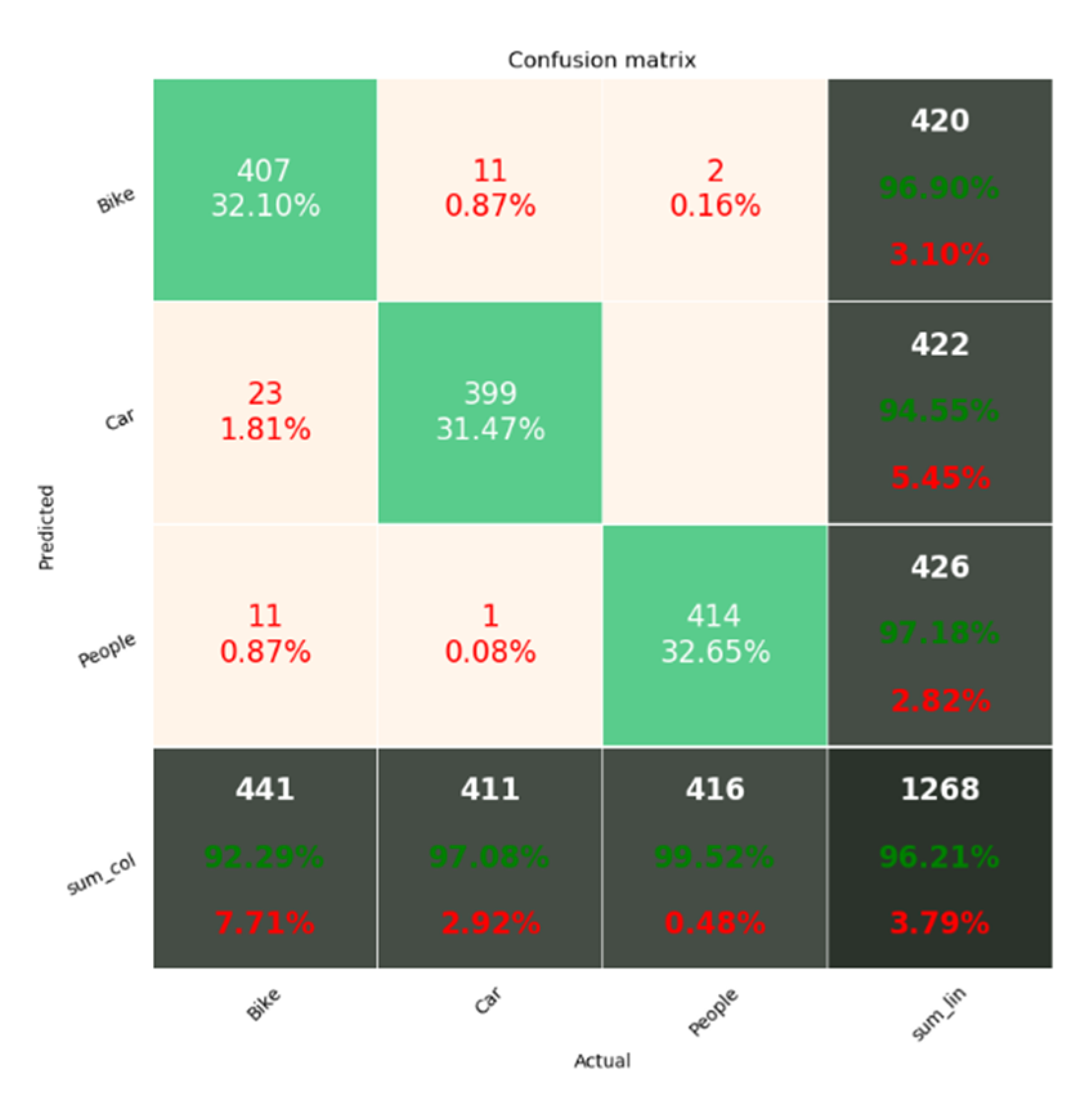
5. Experimental Result

In this section, we compared the experimental results with the proposed algorithm, CNN-based multiple input structure, the results of experimenting with single-channel data and the results of using two-channel data. The computer used in the experiment was the Intel core CPU i9-9900 3.10 GHz, 32 GB RAM and GPU GeForce RTX 2080 SUPER. In all experiments, the categorical cross-entropy function was used for the loss function, Adam [30] for the optimizer and rectified linear unit (ReLU) [31] for the activation function for the three classifications of car, motorcycle and person. The learning rate was 0.0001, the epoch was 100 times and the batch size was 64. Tensorflow framework is used to implement the proposed model [32].

Table 2. Identification results according to approach and number of the input layer.

Approach	Number of Input Layers	Classification Performance	Number of Parameters	Training Time
Range–Doppler map [16]	1	82.26%	16,207	47s
Point cloud map	1	91.32%	16,207	48s
Range–Doppler and point cloud maps	1	92.82%	16,243	54s
Range–Doppler and point cloud maps (3 fully connected layers)	2	95.98%	62,699	63s
Range–Doppler and point cloud maps (1 fully connected layers)	2	96.21%	16,207	56s

shows the number of parameters used for learning and classification performance, according to input data and input structure. When the range–Doppler map was used as a single input, it had 82.26% classification performance. When a point cloud map was used as a single input, the performance was better than when a range–Doppler map was an input, and the accuracy was 91.32%. In the case of the range–Doppler map, there were many data of similar shape between data of cars, people and motorcycle. However, in the case of the point cloud map, the number of similar data was smaller than that of the range–Doppler map. Therefore, it had better identification performance when using the range–Doppler map and the point cloud map as 2 channels as shown in Figure 2 than when using only the range–Doppler map. However, there was no correlation between the range–Doppler map image and the point cloud map image. Therefore, when the proposed multi-input structure was used, the best performance was obtained at 95.98%.

Figure 9 is the confusion matrix of the proposed system. The x-axis is the actual value and the y-axis is the predicted value.

In the case of the motorcycle, the result of misclassification as a person was the most, and conversely, in the case of people, there were many cases of misclassification as a motorcycle. The reason is that in the case of people and motorcycles, there were many similar data in the form of a wide spread of Doppler values in the range–Doppler map. In many cases, cars were misclassified as motorcycles, because in the case of motorcycles and cars, both the range–Doppler map and the point cloud map have similar data in both sizes and shapes. In addition, to reduce the number of trainable parameters, the experiment was conducted by varying the number of fully connected layers. From the results shown in Table 2, although the number of trainable parameters was decreased when some fully connected layers were removed, the model still achieved an accuracy of 96.21%.

6. Conclusions

In this paper, we proposed a multiple-input algorithm for a deep learning-based classification model by collecting radar signals for cars, people and motorcycles. In the experiment, only the basic CNN structure was used considering a real-time operation. The range–Doppler map has a problem that the image changes a lot depending on the angle at which the object faces the radar. Therefore, a point cloud map with a small change in the image according to angle was added as a feature. There are no common features between the distance–Doppler map and the point cloud map. When the two images were input through two channels, it did not have optimal identification performance. Therefore, we proposed a CNN-based multi-input deep learning model and obtained the best identification accuracy.

References

1. Brännström, M.; Coelingh, E.; Sjöberg, J. Model-based threat assessment for avoiding arbitrary vehicle collisions. Trans. Intell. Transp. Syst. 2010, 11, 658–669. [Google Scholar] [CrossRef]
2. Vahidi, A.; Eskandarian, A. Research advances in intelligent collision avoidance and adaptive cruise control. Trans. Intell. Transp. Syst. 2003, 4, 143–153. [Google Scholar] [CrossRef] [Green Version]
3. Han, S.J.; Choi, J. Parking space recognition for autonomous valet parking using height and salient-line probability maps. Etri J. 2015, 37, 1220–1230. [Google Scholar] [CrossRef]
4. Leonard, J.; How, J.; Teller, S.; Berger, M.; Campbell, S.; Fiore, G.; Fletcher, L.; Frazzoli, E.; Huang, A.; Karaman, S.; et al. A perceptiondriven autonomous urban vehicle. J. Field Robot. 2008, 25, 727–774. [Google Scholar] [CrossRef] [Green Version]
5. Yeong, D.J.; Velasco-Hernandez, G.; Barry, J.; Walsh, J. Sensor and sensor fusion technology in autonomous vehicles: A review. Sensors 2021, 21, 2140. [Google Scholar] [CrossRef]
6. Matsunami, I.; Nakamura, R.; Kajiwara, A. Rcs measurements for vehicles and pedestrian at 26 and 79ghz. IEICE Trans. Fundam. Electron. Commun. Comput. Sci. 2016, E99A, 204–206. [Google Scholar] [CrossRef]
7. Prophet, R.; Hoffmann, M.; Vossiek, M.; Strum, C.; Ossowska, A.; Malik, W.; Lubbert, U. Pedestrian classification with a 79 GHz automotive radar sensor. In Proceedings of the 19th International Radar Symposium (IRS), Bonn, Germany, 20–22 June 2018; pp. 1–6. [Google Scholar]
8. Patel, K.; Rambach, K.; Visentin, T.; Rusev, D.; Pfeiffer, M.; Yang, B. Deep learning-based object classification on automotive radar spectra. In Proceedings of the IEEE Radar Conference, Boston, MA, USA, 22–26 April 2019; pp. 1–6. [Google Scholar]
9. Du, L.; Li, L.; Wang, B.; Xiao, J. Micro-doppler feature extraction based on time-frequency spectrogram for ground moving targets classification with low-resolution radar. IEEE Sens. J. 2016, 16, 3756–3763. [Google Scholar] [CrossRef]
10. Lees, W.M.; Wunderlich, A.; Jeavons, P.J.; Hale, P.D.; Souryal, M.R. Deep learning classification of 3.5-GHz band spectrograms with applications to spectrum sensing. IEEE Trans. Cogn. Commun. Netw. 2019, 5, 224–236. [Google Scholar] [CrossRef]
11. Lee, H.R.; Park, J.; Suh, Y.-J. Improving classification accuracy of hand gesture recognition based on 60 GHz FMCW radar with deep learning domain adaptation. Electronics 2020, 9, 2140. [Google Scholar] [CrossRef]
12. Wu, Q.; Gao, T.; Lai, Z.; Li, D. Hybrid SVM-CNN classification technique for human–vehicle targets in an automotive LFMCW radar. Sensors 2020, 20, 3504. [Google Scholar] [CrossRef] [PubMed]
13. Peter, T. Introduction to Radar Target Recognition; The Institution of Engineering and Technology: London, UK, 2005. [Google Scholar]
14. Lim, S.; Yoon, Y.-J.; Lee, J.-E.; Kim, S.-C. Phase-based target classification using neural network in automotive radar systems. In Proceedings of the IEEE Radar Conference (RadarConf), Boston, MA, USA, 22–26 April 2019; pp. 1–6. [Google Scholar]
15. Villeval, S.; Bilik, I.; Gurbuz, S.Z. Application of a 24 GHz FMCW automotive radar for urban target classification. In Proceedings of the IEEE Radar Conference, Cincinnati, OH, USA, 19–23 May 2014. [Google Scholar]
16. Rytel-Andrianik, R.; Samczynski, P.; Gromek, D.; Weilgo, J.; Drozdowicz, J.; Malanowski, M. Micro-range, micro-Doppler joint analysis of pedestrian radar echo. In Proceedings of the IEEE Signal Processing Symposium (SPSympo), Debe, Poland, 10–12 June 2015; pp. 1–4. [Google Scholar]
17. Kim, S.; Lee, S.; Doo, S.; Shim, B. In Moving target classification in automotive radar systems using convolutional recurrent neural networks. In Proceedings of the 26th European Signal Processing Conference (EUSIPCO), Rome, Italy, 3–7 September 2018; pp. 1482–1486. [Google Scholar]
18. Vaishnav, P.; Santra, A. Continuous human activity classification with unscented kalman filter tracking using FMCW radar. IEEE Sens. Lett. 2020, 4, 1–4. [Google Scholar] [CrossRef]
19. Anishchenko, L.; Zhuravlev, A.; Chizh, M. Fall detection using multiple bioradars and convolutional neural networks. Sensors 2019, 19, 5569. [Google Scholar] [CrossRef] [PubMed] [Green Version]
20. Skaria, S.; Al-Hourani, A.; Lech, M.; Evans, R.J. Hand-gesture recognition using two-antenna Doppler radar with deep convolutional neural networks. IEEE Sens. J. 2019, 19, 3041–3048. [Google Scholar] [CrossRef]
21. Kim, Y.; Moon, T. Human detection and activity classification based on micro-Doppler signatures using deep convolutional neural networks. IEEE Geosci. Remote. Sens. Lett. 2015, 13, 8–12. [Google Scholar] [CrossRef]
22. Angelov, A.; Robertson, A.; Murray-Smith, R.; Fioranelli, F. Practical classification of different moving targets using automotive radar and deep neural networks. IET Radar Sonar Navig. 2018, 12, 1082–1089. [Google Scholar] [CrossRef] [Green Version]
23. Lee, S.; Seo, I.; Seok, I.; Seog Han, D. Active sonar target classification with power-normalized cepstral coefficients and convolutional neural network. Appl. Sci. 2020, 10, 8450. [Google Scholar] [CrossRef]
24. Daher, A.W.; Rizik, A.; Randazzo, A.; Tavanti, E.; Chible, H.; Muselli, M.; Caviglia, D.D. Pedestrian and multi-class vehicle classification in radar systems using rulex software on the raspberry pi. Appl. Sci. 2020, 10, 9113. [Google Scholar] [CrossRef]
25. Muselli, M. Extracting knowledge from biomedical data through Logic Learning Machines and Rulex. EMBnet. J. 2012, 18, 56–58. [Google Scholar] [CrossRef]
26. Kim, W.; Cho, H.; Kim, J.; Kim, B.; Lee, S. YOLO-based simultaneous target detection and classification in automotive FMCW Radar Systems. Sensors 2020, 20, 2897. [Google Scholar] [CrossRef]
27. LeCun, Y.; Boser, B.; Denker, J.; Henderson, D.; Howard, R.; Hubbard, W.; Jackel, L. Handwritten digit recognition with a backpropagation network. In Advances in Neural Information Processing Systems; Touretzky, D., Ed.; Morgan-Kaufmann: San Francisco, CA, USA, 1990; Volume 2, pp. 396–404. [Google Scholar]
28. Simonyan, K.; Zisserman, A. Very deep convolutional networks for large-scale image recognition. arXiv 2014, arXiv:1409.1556. [Google Scholar]
29. Zhu, J.; Chen, H.; Ye, W. A hybrid CNN–LSTM network for the classification of human activities based on micro-doppler radar. IEEE Access 2020, 8, 24713–24720. [Google Scholar] [CrossRef]
30. Kingma, D.P.; Ba, J. Adam: A method for stochastic optimization. In Proceedings of the International Conference on Learning Representations (ICLR), San Diego, CA, USA, 7–9 May 2015. [Google Scholar]
31. Nair, V.; Hinton, G.E. Rectified linear units improve restricted boltzmann machines. In ICML’10: Proceedings of the 27th International Conference on International Conference on Machine Learning; Omnipress: Madison, WI, USA, 2010; pp. 807–814. [Google Scholar]
32. Abadi, M.; Agarwal, A.; Barham, P.; Brevdo, E.; Chen, Z.; Citro, C.; Corrado, G.S.; Davis, A.; Dean, J.; Devin, M.; et al. TensorFlow: Large-Scale Machine Learning on Heterogeneous Systems. arXiv 2016, arXiv:1603.04467. [Google Scholar]
Figure 1. Conventional CNN structure as single input.
Electronics 10 01144 g001
Figure 2. Proposed multi-input-based deep learning structure.
Electronics 10 01144 g002
Figure 3. Block diagram of the proposed algorithm.
Electronics 10 01144 g003
Figure 4. Image preprocessing: (a) preprocessing of the point cloud map; (b) preprocessing of the range–Doppler map.
Electronics 10 01144 g004
Figure 5. Experiment environment and object movement path: (a) experiment environment; (b) object movement path.
Electronics 10 01144 g005
Figure 6. Range–Doppler map and point cloud map when a person moves: (a) range–Doppler map when moving diagonally; (b) point cloud map when moving diagonally; (c) range–Doppler map when moving vertically; (d) point cloud map when moving vertically; (e) range–Doppler map when moving horizontally; (f) point cloud map when moving horizontally.
Electronics 10 01144 g006
Figure 7. Range–Doppler map and point cloud map when a car moves: (a) range–Doppler map when moving diagonally; (b) point cloud map when moving diagonally; (c) range–Doppler map when moving vertically; (d) point cloud map when moving vertically; (e) range–Doppler map when moving horizontally; (f) point cloud map when moving horizontally.
Electronics 10 01144 g007
Figure 8. Range–Doppler map and point cloud map when a motorcycle moves: (a) range–Doppler map when moving diagonally; (b) point cloud map when moving diagonally; (c) range–Doppler map when moving vertically; (d) point cloud map when moving vertically; (e) range–Doppler map when moving horizontally; (f) point cloud map when moving horizontally.
Electronics 10 01144 g008
Figure 9. Confusion matrix of proposed system.
Electronics 10 01144 g009